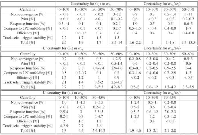
ATLAS-CONF-2012-114 14August2012
ATLAS NOTE
ATLAS-CONF-2012-114
August 12, 2012
Measurement of the distributions of event-by-event flow harmonics in Pb-Pb collisions at √ s
NN= 2.76 TeV
The ATLAS Collaboration
Abstract
The event-by-event distributions of harmonic flow coefficients
vnfor n=2–4 are mea- sured in Pb-Pb collisions at
√sNN =2.76 TeV, using charged particles with p
T >0.5 GeV and in the pseudorapidity range
|η|<2.5. These distributions are obtained by unfolding the raw
vndistributions with a response function that accounts for the smearing of the
vndue to finite number of tracks in the detector acceptance. The shape of the unfolded distribu- tions is found to be consistent with a 2-D Gaussian for the underlying flow vector in central collisions for
v2and over the full centrality range for
v3and
v4; When these distributions are rescaled to the same
hvni, the resulting shapes are found to be nearly the same between
pT <1 GeV and p
T >1 GeV. The
vndistributions are compared with the eccentricity dis- tributions from two initial geometry models: a Glauber model and a model that includes corrections to the initial geometry due to gluon saturation effects. Both models fail to de- scribe the experimental data consistently across the full centrality range. These results may shed light on the nature of the fluctuation of the created matter in the initial state as well as the subsequent hydrodynamic evolution.
c Copyright 2012 CERN for the benefit of the ATLAS Collaboration.
Reproduction of this article or parts of it is allowed as specified in the CC-BY-3.0 license.
1 Introduction
Heavy ion collisions at the Relativistic Heavy Ion Collider (RHIC) and the Large Hadron Collider (LHC) create hot, dense matter that is thought to be composed of strongly coupled quarks and gluons. One strik- ing observation that supports this picture is the large momentum anisotropy of particle emission in the transverse plane. This anisotropy is believed to be the result of anisotropic expansion of the created mat- ter driven by the pressure gradients, with more particles emitted in the direction of the largest gradients.
The collective expansion or flow of the matter can be modelled by relativistic viscous hydrodynamic theory. The magnitude of the azimuthal anisotropy is sensitive to transport properties of the matter, such as the ratio of the shear viscosity to the entropy density and the equation of state [1, 2].
The anisotropy of the particle distribution in azimuthal angle φ is described by a Fourier series:
dN
dφ ∝
1
+2
X∞ n=1v
ncos n(φ
−Φn) (1)
where v
nand
Φnrepresent the magnitude and phase of the n
th-order anisotropy (or flow) at corresponding angular scale (2π/n); they can also be conveniently represented by the per-particle “flow vector” [1]:
⇀
v
n=(v
ncos nΦ
n, v
nsin nΦ
n). The
Φnis referred to as the event plane (EP). The experimentally measured event plane direction
Ψncan smear around
Φndue to the finite number of particles in the event.
Due to the almond-like shape of the overlap region in non-central collisions, the anisotropy is dom- inated by the second harmonic term v
2. However, significant first-order (n=1) and higher-order (n>2) coefficients have also been observed [3–5]. These coefficients are related to additional shape components arising from the fluctuations of the nucleon positions in the overlap region. The amplitudes ǫ
n(or eccen- tricities) and the directions
Φ∗nof these shape components can be estimated via a simple Glauber model from the transverse positions (r, φ) of the participating nucleons relative to their center-of-mass [6]:
ǫ
n=phrn
cos nφ
i2+hrnsin nφ
i2hrni
, tan nΦ
∗n= hrnsin nφ
ihrn
cos nφ
i(2)
The large pressure gradients and ensuing hydrodynamic evolution can convert these shape deformations into higher-order azimuthal anisotropy in the momentum space. For small fluctuations, one expects v
n ∝ǫ
n, and the
Φnto be correlated with the minor-axis direction given by
Φ∗n+π/n. However, model calculations show that the values of ǫ
nare large, and the alignment between
Φnand
Φ∗n+π/n are strongly violated for n > 3 due to non-linear effects in the hydrodynamic evolution [7, 8].
Significant v
ncoefficients for n
≤6 have been measured at the LHC [3–5]. Strong correlations are also observed for many combinations of two or three
Φnof different order [9]. These findings are consistent with the existence of sizable fluctuations in the initial state and strong non-linear effects in the final state [8, 10]. More information on these fluctuations and non-linear effects can be obtained by measuring the v
non an event-by-event (EbE) basis, which gives the probability distribution for each v
n. This is the aim of the analysis presented here. Some properties of the v
ndistributions were previously inferred using the two- and four-particle cumulant methods, with the measured coefficients denoted as v
n{2
}and v
n{4
}[11, 12], respectively. In the limit of Gaussian distribution for the underlying flow vector, they are related to the mean and the standard deviation of the v
n[11]:
v
n{2
}2=hv
ni2+σ
2vn
, v
n{4
}2=hv
ni2−σ
2vn
(3)
The relative width of the distribution, defined as σ
vn/
hv
ni, was measured [13, 14] to be about 0.3-0.5 for
n=2 depending on centrality. However, these indirect measurements rely on the assumption that the flow vector follows a 2-D Gaussian distribution and hence are subject to significant systematic uncertainty.
In contrast, these and many additional quantities such as kurtosis and skewness can be obtained directly
from the actual v
ndistributions. The key step in this measurement is to unfold the observed v
ndistribution for the smearing due to the effect of finite per-event charged particle multiplicity. This measurement is possible in ATLAS, due to its large detector acceptance and the large particle multiplicities produced in lead-lead collisions at the LHC.
2 ATLAS detector and trigger
The ATLAS detector [15] provides nearly full solid angle coverage of the collision point with track- ing detectors, calorimeters and muon chambers, which are well suited for measurements of azimuthal anisotropies over a large pseudorapidity range
1. This analysis primarily uses two subsystems: the inner detector (ID) and the forward calorimeter (FCal). The ID is contained within the 2 T field of a supercon- ducting solenoid magnet, and measures the trajectories of charged particles in the pseudorapidity range
|
η
|< 2.5 and over the full azimuth. A charged particle passing through the ID traverses typically three modules of the silicon pixel detector (Pixel), four double-sided silicon strip modules of the semiconduc- tor tracker (SCT), and a transition radiation tracker for
|η
|< 2. The FCal consists of three longitudinal sampling layers and covers 3.2 <
|η
|< 4.9. In heavy ion collisions the FCal is used mainly to measure the event centrality and event planes [5, 16].
The minimum-bias Level-1 trigger used for this analysis requires signals in two zero-degree calorime- ters (ZDC), each positioned at 140 m from the collision point, detecting neutrons and photons with
|η
|>
8.3, or either one of the two minimum-bias trigger scintillator (MBTS) counters, covering 2.1 <
|η
|< 3.9 on each side of the nominal interaction point. The ZDC Level-1 trigger thresholds on each side are set below the peak corresponding to a single neutron. A Level-2 timing requirement based on signals from each side of the MBTS is imposed to remove beam backgrounds.
3 Event and track selections
This analysis is based on approximately 8 µb
−1of Pb-Pb data collected in 2010 at the LHC with a nucleon-nucleon center-of-mass energy
√sNN =2.76 TeV. An offline event selection requires a recon- structed vertex and a time difference
|∆t|< 3 ns between the MBTS trigger counters on either side of the interaction point to suppress non-collision backgrounds. A coincidence between the ZDCs at forward and backward pseudorapidity is required to reject a variety of background processes, while maintaining high efficiency for non-Coulomb processes. Events satisfying these conditions are required to have a reconstructed primary vertex within
|zvtx|< 150 mm of the nominal center of the ATLAS detector.
The Pb-Pb event centrality [17] is characterized using the total transverse energy (
PET
) deposited in the FCal over the pseudorapidity range 3.2 <
|η
|< 4.9 at the electromagnetic energy scale [18].
An analysis of this distribution after all trigger and event selections gives an estimate of the fraction of the sampled non-Coulomb inelastic cross-section to be 98
±2%. The uncertainty associated with the centrality definition is evaluated by varying the effect of trigger and event selection inefficiencies as well as background rejection requirements in the most peripheral FCal
PET
interval [17]. The FCal
P ETdistribution is divided into a set of 5% percentile bins, together with five 1% bins for the top 5% most central events. A standard Glauber Monte-Carlo analysis [17, 19] is used to estimate the average number of participating nucleons,
hNparti, for each centrality interval. These numbers are summarized in Table 1.
The v
ncoefficients are measured with the ID, using reconstructed tracks with p
T> 0.5 GeV and
|
η
|< 2.5. At least nine hits in the silicon detectors (out of a typical value of 11) are required for each
1ATLAS uses a right-handed coordinate system with its origin at the nominal interaction point (IP) in the center of the detector and the z-axis along the beam pipe. The x-axis points from the IP to the center of the LHC ring, and they-axis points upward. Cylindrical coordinates (r, φ) are used in the transverse plane,φbeing the azimuthal angle around the beam pipe. The pseudorapidity is defined in terms of the polar angleθasη=−ln tan(θ/2).
Centrality 0-1% 1-2% 2-3% 3-4% 4-5%
hNparti
400.6
±1.3 392.6
±1.8 383.2
±2.1 372.6
±2.3 361.8
±2.5
Centrality 0-5% 5-10% 10-15% 15-20% 20-25%
hNparti
382.2
±2.0 330.3
±3.0 281.9
±3.5 239.5
±3.8 202.6
±3.9
Centrality 25-30% 30-35% 35-40% 40-45% 45-50%
hNparti
170.2
±4.0 141.7
±3.9 116.8
±3.8 95.0
±3.7 76.1
±3.5
Centrality 50-55% 55-60% 60-65% 65-70%
hNparti
59.9
±3.3 46.1
±3.0 34.7
±2.7 25.4
±2.3
Table 1: The relationship between centrality interval and the
hNpartiestimated from the Glauber model.
track, with no missing Pixel hits and not more than one missing SCT hit, taking into account the effects of known dead modules. In addition, the point of closest approach of the track is required to be within 1 mm of the primary vertex in both the transverse and longitudinal directions [16]. The tracking efficiency is studied by comparing data to Monte Carlo calculations based on the HIJING event generator [20] and a full GEANT4 [21] simulation of the detector. The track reconstruction efficiency in central events is estimated to be about 70% near mid-rapidity and decreases to 50% at forward rapidity [22].
4 Methodology
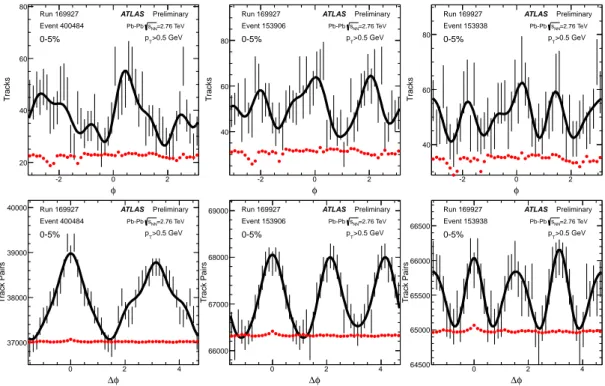
To illustrate the level of EbE fluctuations in the data, the top panels of Figure 1 show the azimuthal distribution of charged tracks with p
T> 0.5 GeV for three central events. The corresponding pair
∆φdistributions from the same events are shown in the bottom panels. For each pair of particles two
∆φentries,
|φ
1−φ
2|and
−|φ
1−φ
2|, are made each with a weight of 1/2, and then folded into [-0.5π,1.5π]
interval. Both distributions are overlaid with the acceptance functions (arbitrary normalization). Rich EbE patterns, beyond the structures seen in the acceptance functions (solid points), are observed. These distributions are the inputs for the EbE v
nanalyses.
The azimuthal distribution of charged particles in a given event can be expanded into a Fourier series:
dN
dφ ∝
1
+2
X∞ n=1v
obsncos n(φ
−Ψobsn)
=1
+2
X∞n=1
v
obsn,xcos nφ
+v
obsn,ysin nφ)
(4) v
obsn =r
v
obsn,x2+
v
obsn,y2, tannΨ
obsn =v
obsn,yv
obsn,x, v
obsn,x =hcos nφ
i, v
obsn,y =hsin nφ
i, (5) where the averages are over all particles in the event for the required η range. The v
obsnis the magnitude of the observed per-particle flow vector:
⇀v
nobs =(v
obsn,x, v
obsn,y). In the limit of infinite multiplicity and the absence of non-flow effects, it should approach the true flow signal: v
obsn →v
n. The key issue in measuring the EbE v
nis to determine the response function p(v
obsn |v
n), which is then used to unfold the smearing effect due to finite number of detected particles. Possible non-flow effects from short-range correlations, such as resonance decays, Bose-Einstein correlation and jets, also need to be suppressed.
The rest of this section sets out the steps to obtain the unfolded v
ndistribution. Section 4.1 explains
how the data are corrected for detector acceptance to obtain
⇀v
obsn, and then how the response function
is obtained from correlation of
⇀v
obsnbetween two symmetric subevents. Section 4.2 describes how v
ncan be obtained from two-particle correlation (2PC) as shown in lower panels of Figure 1, and how
the associated response function is obtained. In this analysis the 2PC approach is used primarily as a
consistency check (Section 5). The Bayesian unfolding procedure, applicable to either the single particle
or 2PC data, is described in Section 4.3. The performance of the unfolding and systematics follows in
Section 5.
4.1 Single particle method
In an actual experiment, the azimuthal distribution of particles in Figure 1 needs to be corrected for the non-uniform detector acceptance. This is achieved by dividing the foreground distribution (S) of a given event with the acceptance function (B) obtained from all tracks in all events (see top panels of Figure 1):
dN
dφ ∝C(φ)= S (φ)
B(φ) =
1
+2
P∞n=1
v
rawn,xcos nφ
+v
rawn,ysin nφ) 1
+2
P∞n=1
v
detn,xcos nφ
+v
detn,ysin nφ) . (6) v
rawn,x =P
i
(cos nφ
i) /ǫ(η
i,
pT,i)
Pi
1/ǫ(η
i,
pT,i)
= h(cos nφ)/ǫ
ih
1/ǫ
i, v
rawn,y = h(sin nφ)/ǫ
ih
1/ǫ
i, (7)
where ǫ(η,
pT) is the tracking efficiency [22] and v
detn,xand v
detn,yare Fourier coefficients of the acceptance function in azimuth, also weighted by the inverse of the tracking efficiency. Since the azimuthal variation of efficiency corrections are generally small (see Figure 1), the harmonic coefficients are obtained as:
v
obsn,x ≈v
rawn,x −v
detn,x, v
obsn,y ≈v
rawn,y −v
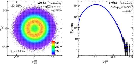
detn,y(8) Figure 2 shows the EbE distribution of per-particle flow vector
⇀v
2obs =(v
obs2,x, v
obs2,y) and v
obs2obtained for tracks at p
T> 0.5 GeV in the 20-25% centrality interval. The azimuthal symmetry in the left panel reflects the random orientation of
⇀v
2obsevent to event. Due to finite track multiplicity, the measured flow vector is smeared randomly around the true flow vector by a 2-D response function p(
⇀v
nobs|⇀v
n).
φ
-2 0 2
Tracks
20 40 60 80
0-5%
ATLAS Preliminary
=2.76 TeV sNN Pb-Pb
>0.5 GeV pT
Run 169927 Event 400484
φ
-2 0 2
Tracks
40 60
80 0-5%
ATLAS Preliminary
=2.76 TeV sNN Pb-Pb
>0.5 GeV pT
Run 169927 Event 153906
φ
-2 0 2
Tracks
40 60
80 0-5%
ATLAS Preliminary
=2.76 TeV sNN Pb-Pb
>0.5 GeV pT
Run 169927 Event 153938
φ
∆
0 2 4
Track Pairs
37000 38000 39000 40000
0-5%
ATLAS Preliminary
=2.76 TeV sNN Pb-Pb
>0.5 GeV pT
Run 169927 Event 400484
φ
∆
0 2 4
Track Pairs
66000 67000 68000 69000
0-5%
ATLAS Preliminary
=2.76 TeV sNN Pb-Pb
>0.5 GeV pT
Run 169927 Event 153906
φ
∆
0 2 4
Track Pairs
64500 65000 65500 66000 66500
0-5%
ATLAS Preliminary
=2.76 TeV sNN Pb-Pb
>0.5 GeV pT
Run 169927 Event 153938
Figure 1: Single track φ (top) and track pair
∆φ(bottom) distributions for three events (from left to right) in 0-5% centrality interval. The pair distributions have been folded into [-0.5π,1.5π]. The bars indicate the foreground distributions, the solid curves indicate a Fourier parameterization including first six harmonics: dN/dφ
= A(1+2
P6i=1cn
cos n(φ
−Ψn)) for single distributions and dN/d∆φ
= A(1+2
P6i=1cn
cos n(∆φ)) for pair distributions, and the red solid points indicate the acceptance functions.
Tracks with p
T> 0.5 GeV are used.
obs
v2,x
-0.2 0 0.2
obs 2,yv
-0.2 0 0.2
0 100 200 300 20-25% ATLAS Preliminary
=2.76 TeV sNN
Pb-Pb
b-1
µ
int= 8 L
obs
v2
0 0.1 0.2 0.3
Events
1 10 102
103
104 ATLAS Preliminary
=2.76 TeV sNN
Pb-Pb
b-1
µ
int= 8 L
> 0.5 GeV pT
Figure 2: The distribution of per-particle flow vector
⇀v
2obs(left panel) and the magnitude v
obs2(right panel) for events in 20-25% centrality interval.
)b obs
-(v2,x
)a obs
(v2,x
-0.2 0 0.2
b )obs 2,y-(va )obs 2,y(v
-0.2 0 0.2
0 500 1000 ATLAS Preliminary
=2.76 TeV sNN Pb-Pb
b-1 µ int= 8 L
20-25%
)b obs
-(v2,x
)a obs
(v2,x
-0.2 0 0.2
Events
1 10 102
103
104
/DOF=1.05 χ2
=0.05039 δ2SE
20-25%
ATLAS Preliminary
=2.76 TeV sNN Pb-Pb
b-1 µ int= 8 L
)b obs
-(v2,y
)a obs
(v2,y
-0.2 0 0.2
Events
1 10 102
103
104
/DOF=1.03 χ2
=0.05018 δ2SE
20-25%
ATLAS Preliminary
=2.76 TeV sNN Pb-Pb
b-1 µ int= 8 L
a) b) c)
> 0.5 GeV
T
p
Figure 3: (left) The distribution of the difference between the per-particle flow vectors of the two half- IDs for events in 20-25% centrality interval. (middle) The projection on to the x-axis overlaid with a fit to a Gaussian. (right) The projection on to the y-axis overlaid with a fit to a Gaussian. The width from the fit, δ
2SE, and the quality of the fit, χ
2/DOF are shown.
In order to determine p(
⇀v
nobs|⇀v
n), the tracks in the ID is divided into two subevents with symmetric η range, η > 0 and η < 0, which have nearly the same average track multiplicity (agree within 1%).
The distribution of flow vector differences between the two subevents, p
sub(
⇀v
nobs)
a−(
⇀v
nobs)
b, is then
obtained in Figure 3a. The physical flow signal cancels in this distribution such that it contains mainly
the effect of statistical smearing. Figure 3b-c show the x and y projections of this residual distribution,
together with fits to a Gaussian function. The fits describe the data across five orders of magnitude
with the same widths, δ
2SE ≈0.050, along both directions with χ
2/DOF
∼1, implying that the smearing
effect is purely statistical. This would be the case if either non-flow effects are small and the smearing is
mostly driven by finite multiplicity, or the number of sources responsible for short-range correlations are
proportional to the multiplicity and they are not correlated between the subevents. The latter could be true
for resonance decays, Bose-Einstein correlation, and jets. Similar behavior is observed for all harmonics
up to centrality interval 50-55%. Beyond that the distributions are more appropriately described by the
Student’s t-distribution, which is a general PDF for the difference between two independent sample-
estimates of the mean. The t-distribution approaches a Gaussian distribution when the number of tracks
is large.
Denoting the width of these 1-D distributions as δ
2SE, then the widths of the 2-D response functions for the half-ID and the full-ID should be δ
2SE/
√2 and δ
2SE/2, respectively; they can be obtained by rescaling Figure 3a in both dimensions by a constant factor c: p(
⇀v
nobs|⇀v
n)
= cpsubch
(
⇀v
nobs)
a−(
⇀v
nobs)
bi, with c
=2 and
√2 for the full-ID and half-ID, respectively. A simple shift of this 2-D distribution to
⇀v
n =(v
n,x, v
n,y), followed by an integration over the azimuthal angle, gives the desired 1-D response function [11, 14, 23]:
p(vobsn |
v
n)
∝v
obsn e−(vobs n )2+v2
n 2δ2 I0
v
obsnv
nδ
2!
, δ
=(
δ
2SE/
√2 for half-ID δ
2SE/2 for full-ID
(9) where I
0is the modified Bessel function of the first kind and the difference s
=v
obsn −v
nis entirely due to the statistical smearing. This analytical function, commonly referred to as the Bessel-Gaussian func- tion [11], can be used to directly unfold the v
obsndistribution, i.e. the right panel of Figure 2. Alternatively, the actual measured distribution p(v
obsn |v
n) taking into account sample statistics, can be directly used in the unfolding. This approach is more suitable for peripheral collisions where the analytical description Eq. 9 is not precise.
4.2 Two-particle correlation method
The unfolding based on EbE two-particle correlation method starts with Eq. 6. An EbE pair distribution is obtained by convolving the tracks in the first half-ID with those in the second half-ID:
dN d∆φ ∝
1
+2
Xn
v
obsn,x1cos nφ
1+v
obsn,y1sin nφ
1
⊗
1
+2
Xn
v
obsn,x2cos nφ
2+v
obsn,y2sin nφ
2
=
1
+2
Xn
h
v
obsn,x1v
obsn,x2 +v
obsn,y1v
obsn,y2cos n∆φ
+v
obsn,x1v
obsn,y2 −v
obsn,y1v
obsn,x2sin n∆φ
i≡
1
+2
Xn
(A
ncos n∆φ
+Bnsin n∆φ) (10)
where the tracking efficiency re-weighting has been applied for v
n,xand v
n,yfor each track similar to Eq. 6. An EbE pair variable v
obsn,nis subsequently calculated:
v
obsn,n = qA2n+B2n= r
v
obsn,x12+
v
obsn,y12v
obsn,x22+
v
obsn,y22=
v
obsn 1v
obsn 2. (11) The observed flow signal from correlation analysis is defined as:
v
obs,2PCn = qv
obsn,n = qv
obsn 1v
obsn 2 = p(v
n+s1)(v
n+s2) (12) where s
1=v
obsn 1−v
nand s
2=v
obsn 2−v
nare independent variables described by the probability distribution in Eq. 9 with δ
=δ
2SE/
√2. The response function for v
obs,2PCnis very different from that for the single particle, but nevertheless can be either calculated analytically via Eq. 9 or generated from the measured distributions in Figure 3. For small v
nvalues, the s
1s2term dominates Eq. 12 and the distribution of v
obs,2PCnis broader than v
obsn. For large v
nvalues, s
1and s
2are approximately Gaussian and hence:
v
obs,2PCn ≈ qv
2n+v
n(s
1+s2)
≈v
n+ s1+s22
=v
n+s1/
√2
=v
n+s(13)
where we have use the fact that the average of two Gaussian random variable is equivalent to a Gaussian with a narrower width, and that the smearing of flow vector for the half-IDs (s
1and s
2) is
√2 broader than that for the full-ID (s). Hence the distribution of v
obs,2PCnis expected to approach the v
obsndistribution of the full-ID when v
n≫δ
2SE/
√2.
4.3 Unfolding
In this analysis, the standard Bayesian unfolding procedure [24], as implemented in the RooUnfold framework [25], is used to calculate the unfolded distribution. The true distribution (“cause” c or v
n) and the measured distribution (“effect” e or v
obsnor v
obs,2PCn) are related via the response function A, which gives the probability that a cause c
iis mapped on to a measured value e
j:
Ac=e, Aji= p(ej|ci
) (14)
The distribution of c is obtained via an iterative pseudo-inversion procedure: An unfolding matrix ˆ
M0is determined from the response function and some initial guess of the true distribution ˆc
0(called a prior):
ˆc
iter+1= Mˆ
itere, Mˆ
i jiter= Ajiˆc
iteri Pm,kAmiAjk
ˆc
iterk(15)
The ˆ
M0is used to calculate the unfolded distribution ˆc
1, which is then used to calculate ˆ
M1and so on.
More iterations reduce the dependence on the prior and gives results closer to the true distributions but with increased statistical fluctuations. So the number of iteration N
iterneeds to be adjusted according to the sample statistics and binning. The prior can be chosen as the v
obsndistribution from the full-ID for the single particle unfolding, and as the v
obs,2PCndistribution from the two half-IDs for the 2PC unfolding.
However, more realistic priors can be obtained by rescaling the input distributions by a constant factor R to obtain a distribution with a mean that is closer to that for the true distribution:
v
obsn →Rvobsn,
R=v
EPn hv
obsn i1 1
+q
1
+σ
obsvn/
hv
obsn i2−
1
! f
,
f =0, 0.5, 1, 1.5, 2, 2.5 . (16)
where
hv
obsn iand σ
obsvn
are the mean and the RMS width of the v
obsndistribution, respectively, and v
EPnis measured using the FCal EP method from [5] with the same track selection criteria for the same dataset.
This rescaling is applied to v
obsnon a EbE basis such that the bin size of the resulting distribution remains unchanged. The EP method in general is known to measure a value in between the simple average and the RMS average of the true v
n[26, 27]:
h
v
ni ≤v
EPn ≤ qh
v
2ni= qh
v
ni2+σ
2vn. (17)
The lower limit is reached when the resolution factor [5] used in the EP method is one, while the upper limit is reached when the resolution factor is close to zero. If the EbE
⇀v
ndistribution is purely Gaussian, it can be shown that [28]:
q
h
v
2ni=2
√
π
hv
ni=1.13
hv
ni, σ
vn hv
ni =r
4
π
−1
=0.523 (18)
Gaussian fluctuations are expected to dominate the v
2in the most central collisions, and more generally for the higher-order harmonics. Thus f
=0 (default choice) gives a prior that is slightly broader than the true distribution; f
=1 gives a distribution that has a mean close to the true distribution; f > 1 typically gives a distribution that is narrower than the true distribution.
The unfolding problem in this analysis has several features that improves its performance:
1. The response function is obtained entirely from the data itself, with no need for Monte Carlo input.
2. Each event provides one entry for the v
obsndistribution and the response function (no efficiency loss), and these distributions can be determined with great precision (about 2.4 million events for each 5% centrality interval).
3. The unfolded v
ndistribution is always narrower than the v
obsndistribution, hence there is no leakage
problem.
5 Unfolding performance and systematic uncertainties
This section describes the unfolding of the single particle distribution (Eq. 4) and summarizes a series of checks to verify the robustness of the results: a) the number of iterations used, b) comparison with results obtained from a smaller η range, c) variation of the initial prior, d) comparison with the results obtained by unfolding the 2PC distribution, and e) checking for bias due to non-flow, short-range correlations by varing the η gap between the two half-IDs. Only a small subset of the available figures is presented here;
a wider selection can be found in the Appendix.
5.1 Unfolding performance
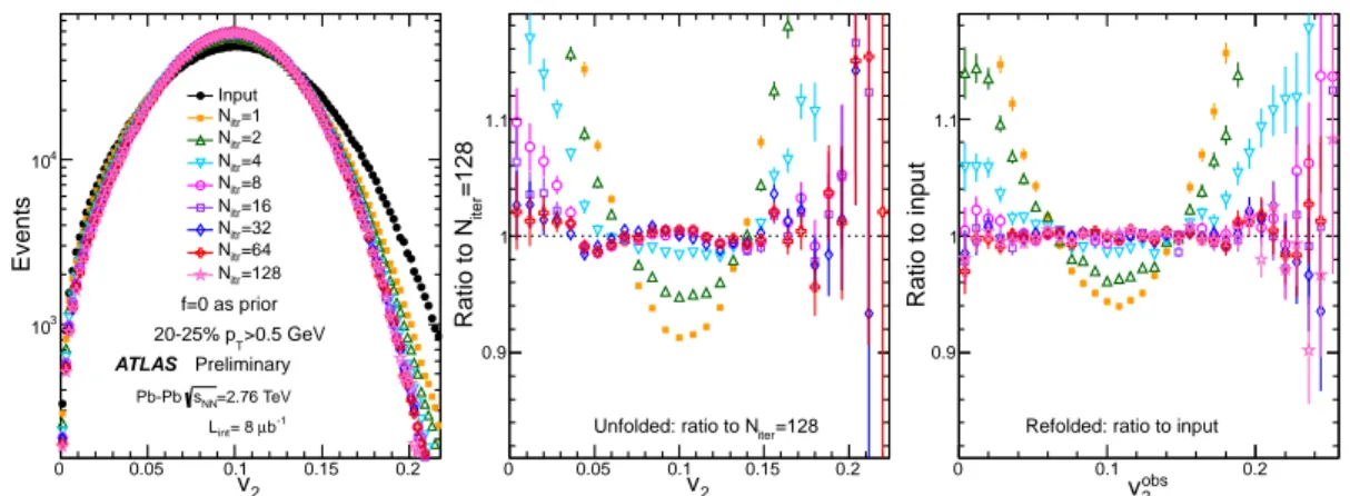
Figure 4 shows the convergence behavior of single particle unfolding for v
2in the 20-25% centrality interval measured with the full-ID. The results converge to within a few percent by N
iter =4 around the peak of the distribution, but the convergence is slower in the tails and there are small, systematic improvements at the level of a few percent for N
iter ≥8. The refolded distributions, obtained by con- volving the unfolded distributions with the response function, indicate that the convergence is reached for N
iter ≥8. Figures 5 and 6 shows similar distributions for v
3and v
4. The unfolding performances are similar to that shown in Figure 4, except that the tails of the unfolded distributions require more iterations to converge. For example, Figure 6 suggests that the bulk region of the distributions, both unfolded and refolded, have converged by N
iter =32, but the tails still exhibit some small changes up to N
iter =64.
The slower convergence for higher-order harmonics simply reflects the fact that the physical v
nsignal is smaller for larger n, while the values of δ
2SEchange only weakly with n. These studies are repeated for all centrality intervals. In general, more iterations are needed for peripheral collisions due to the increase of δ
2SE.
v2
0 0.05 0.1 0.15 0.2
Events
103
104
>0.5 GeV 20-25% pT
f=0 as prior Input
itr=1 N
itr=2 N
itr=4 N
itr=8 N
itr=16 N
itr=32 N
itr=64 N
itr=128 N
ATLAS Preliminary
=2.76 TeV sNN
Pb-Pb b-1
µ
int= 8 L
v2
0 0.05 0.1 0.15 0.2
=128iterRatio to N
0.9 1 1.1
iter=128 Unfolded: ratio to N
obs
v2
0 0.1 0.2
Ratio to input
0.9 1 1.1
Refolded: ratio to input
Figure 4: The performance of unfolding of v
2for the 20-25% centrality interval (left panel) for various
Niter, and the ratios of the unfolded distributions to the results after 128 iterations (middle panel). The ratios of the refolded distributions to the input v
obs2are shown in the right panel.
The statistical uncertainties given by the unfolding procedure are verified via a resampling tech- nique [29]. For small N
iter, the statistical uncertainties as given by diagonal entries of the covariance matrix are much smaller than
√N, where N is the number of entries in each bin, indicating the presence
of statistical bias of the prior. But these uncertainties increase with N
iter, and generally approach
√N
for 64
≤ Niter ≤128. In this analysis, the centrality range for each harmonic n is chosen such that the convergence is reached for N
iter≥64, defined as the difference between N
iter =64 and N
iter=128 to be less than 5% in any bin when statistics allows. They are 0-70% for v
2, 0-60% for v
3and 0-45% for v
4.
The robustness of the unfolding procedure is checked by comparing the results measured indepen-
dently for the half-ID and the full-ID. The results are shown in Figure 7. Despite the large differences
v3
0 0.05 0.1
Events
103
104
105
>0.5 GeV 20-25% pT
f=0 as prior
Input
itr=1 N
itr=2 N
itr=4 N
itr=8 N
itr=16 N
itr=32 N
itr=64 N
itr=128 N
ATLAS Preliminary
=2.76 TeV sNN
Pb-Pb b-1
µ
int= 8 L
v3
0 0.05 0.1
=128iterRatio to N
0.9 1 1.1
iter=128 Unfolded: ratio to N
obs
v3
0 0.05 0.1 0.15
Ratio to input
0.9 1 1.1
Refolded: ratio to input
Figure 5: The performance of unfolding of v
3for the 20-25% centrality interval (left panel) for various
Niter, and the ratios of the unfolded distributions to the results after 128 iterations (middle panel). The ratios of the refolded distributions to the input v
obs3are shown in the right panel.
v4
0 0.02 0.04 0.06
Events
103
104
105
>0.5 GeV 20-25% pT
f=0 as prior
Input
itr=1 N
itr=2 N
itr=4 N
itr=8 N
itr=16 N
itr=32 N
itr=64 N
itr=128 N
ATLAS Preliminary
=2.76 TeV sNN
Pb-Pb b-1
µ
int= 8 L
v4
0 0.02 0.04 0.06
=128iterRatio to N
0.9 1 1.1
iter=128 Unfolded: ratio to N
obs
v4
0 0.05 0.1
Ratio to input
0.9 1 1.1
Refolded: ratio to input
Figure 6: The performance of unfolding of v
4for the 20-25% centrality interval (left panel) for various
Niter, and the ratios of the unfolded distributions to the results after 128 iterations (middle panel). The ratios of the refolded distributions to the input v
obs4are shown in the right panel.
in their initial distributions, the final unfolded results agree to within a few percent in the bulk region of the unfolded distribution. Systematic differences are observed in the tails of the distributions for v
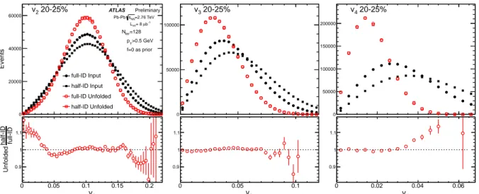
4, especially in peripheral collisions, with the half-ID results being slightly broader. This behavior reflects mainly the residual non-convergence of the half-ID, since its response function is a factor of
√2 broader than that for the full-ID.
A wide range of priors are tried in this analysis, including the measured v
obsndistribution and the six rescaled distributions defined by Eq. 16. Figure 8 compares the convergence behavior of these priors for v
4in the 20-25% centrality interval. Despite the significantly different initial distributions, the unfolded distributions all converge to the same answer for N
iter ≥64 within their respective statistical errors.
However, the convergence is faster with an appropriate choice of priors. Furthermore, choosing a prior that is narrower than the unfolded distribution leads to convergence in one direction, and a broader prior converges from the other direction. Taken together, this allows a quantitative evaluation of the residual non-convergence in the unfolded distributions.
Figure 9 compares the convergence behavior between unfolding of single particle v
obsnand unfolding
of 2PC v
obs,2PCnin 20-25% centrality interval with f
=0 prior. Despite very different response functions
and initial distributions, the unfolded results agree with each other to within a few percent in the bulk
region of the unfolded distribution. The systematic deviations in the tails of the v
4distribution (bottom-
v
Events
0 20000 40000 60000
full-ID Input half-ID Input full-ID Unfolded half-ID Unfolded
f=0 as prior ATLAS Preliminary
=2.76 TeV sNN Pb-Pb
b-1 µ int= 8 L iter=128 N
>0.5 GeV pT
20-25%
v2
0 v
50000 100000
20-25%
v3
0 v
50000 100000 150000 200000
20-25%
v4
v2
0 0.05 0.1 0.15 0.2
full-IDhalf-IDUnfolded 0.9
1 1.1
v3
0 0.05 0.1
0.9 1 1.1
v4
0 0.02 0.04 0.06
0.9 1 1.1
Figure 7: Comparison of the input distributions (solid symbols) and unfolded distributions for N
iter=128 (open symbols) between the half-ID and full-ID in 20-25% centrality interval. The ratios between the unfolded results for half-ID and full-ID are shown in the bottom panels. The results are shown for v
2(left), v
3(middle) and v
4(right).
v
Events
102
103
104
105
Input f=0 f=0.5 f=1 f=1.5 f=2 f=2.5 Final result
Prior 20-25%
>0.5 GeV pT
v
iter=8 N
Single particle unfolding
ATLAS Preliminary
=2.76 TeV sNN Pb-Pb
b-1 µ int= 8 L
v
iter=32 N
v
iter=64 N
v
iter=128 N
v4
0 0.02 0.04 0.06
Ratio
0.9 1 1.1
v4
0 0.02 0.04 0.06
v4
0 0.02 0.04 0.06
v4
0 0.02 0.04 0.06
v4
0 0.02 0.04 0.06