ATLAS-CONF-2016-105 29September2016
ATLAS NOTE
ATLAS-CONF-2016-105
20th September 2016
Measurement of the azimuthal anisotropy of charged particles produced in 5.02 TeV Pb + Pb collisions with the ATLAS detector
The ATLAS Collaboration
Abstract
The data collected by the ATLAS experiment during the 2015 heavy ion LHC run offers new opportunities to probe properties of the Quark-Gluon Plasma at unprecedented high temperatures and densities. Study of the azimuthal anisotropy of produced particles not only constrains our understanding of initial conditions of nuclear collisions and soft particle collective dynamics, but also sheds light on jet-quenching phenomena via measurement of flow harmonics at high transverse momenta. A new ATLAS measurement of elliptic flow and higher-order Fourier harmonics of charged particles in Pb
+Pb collisions at
√s
NN=5.02 TeV in a wide range of transverse momenta, pseudorapidity (|η|
<2.5) and collision centrality is presented. These measurements are based on the Scalar Product and Two Particle Correlation methods. The measurements are compared with the results for Pb+Pb collisions at the lower energy.
c
2016 CERN for the benefit of the ATLAS Collaboration.
Reproduction of this article or parts of it is allowed as specified in the CC-BY-4.0 license.
1 Introduction
The properties of the QGP have been under thorough investigation since its discovery in Au+Au colli- sions at the Relativistic Heavy Ion Collider (RHIC) [1–4]. The existence of the Quark-Gluon Plasma (QGP) phase of nuclear matter, predicted by the Quantum Chromodynamics lattice calculations [5], has been confirmed by a wealth of experimental data. In particular, the properties related to the collective expansion of the QGP (e.g. the equation of state and shear viscosity) are inferred from measurements of azimuthal anisotropies of produced particles. It is expected that the azimuthal anisotropy results from large initial pressure gradients in the hot, dense matter created in the collisions. These pressure gradi- ents transform the initial spatial anisotropies of nuclear collisions into momentum anisotropies of the final-state particle production, which are experimentally characterised by Fourier (flow) harmonics of the azimuthal angle distributions of produced particles [6, 7]. The discovery of large flow harmonics at RHIC, and more recently at much higher collision energy at the LHC [8–11], has significantly deepened our understanding of the QGP. In particular, the recent measurements of azimuthal anisotropy help to constrain the commonly used modelling of the dynamics of heavy-ion collisions based on relativistic vis- cous hydrodynamics. The hydrodynamic models assume that, shortly after the collision, the system is in a local equilibrium and forms a strongly interacting quark-gluon medium. Detailed investigations, based on hydrodynamics, have shown that the produced medium has properties similar to an almost ideal liquid characterised by a very low ratio of viscosity to entropy density,
η/s. The goal of experimental heavy-ionphysics is to improve our understanding of the strongly coupled QGP. Precise flow measurements are central to this because of their unique sensitivity to
η/s.The anisotropic distribution of azimuthal angles of produced particles is expanded as a Fourier series [12, 13]:
dN dφ
=N
02π
1
+Xn=1
2v
ncos
n (φ
−Φn)
,
(1)
where
φis the azimuthal angle of the produced particles and the
vnand
Φnare the magnitude and orienta- tion of the n
thorder azimuthal anisotropy. The coefficients,
vn, are commonly called “flow harmonics” due to their hydrodynamic origin. The
vncoe
fficients are functions of particle pseudorapidity (η), transverse momentum (p
T), and the degree of overlap between the colliding nuclei (centrality). Both the size of the collision overlap region and, for a given size, the number of interacting nucleons fluctuate from event to event. This generates so-called anisotropic flow fluctuations which arise from the initial fluctuations of the overlap region.
The first harmonic,
v1, is known as directed flow and refers to the sideward motion of fragments in ultra- relativistic nuclear collisions, and it carries information from the early stage of the collision. The most extensive studies are related to the second flow harmonic
v2, also known as elliptic flow. Elliptic flow is sensitive to the initial spatial asymmetry of the almond-shaped overlapping zone of colliding nuclei. The higher-order coe
fficients
vn, n
>2 are also important due to their sensitivity to the initial state geometry fluctuations and viscosity e
ffects.
During the first operational period at the LHC (Run 1) Pb ions were collided at energy per nucleon
√
s
NN=2.76 TeV, which is about 13 times larger than the highest collision energy attained at RHIC
in Au+Au collisions. ATLAS and other LHC experiments collected large samples of heavy-ion data
allowing for extensive studies of the elliptic flow and higher-order Fourier coefficients. ATLAS meas-
urements of flow harmonics were performed in broad regions of transverse momentum, pseudorapidity
and event centrality, using the standard event-plane (EP) method [9], two-particle correlation function
(2PC) [10] and multi-particle cumulants [14]. Significant (non-zero) flow harmonics
vnup to n
=6 were measured in Pb+Pb collisions at energy
√s
NN=2.76 TeV, which indicate a very low shear viscosity ofthe QGP medium. Additionally, by comparing RHIC (STAR [15] and PHENIX [16]) and LHC (ATLAS [9], ALICE [17] CMS [18]) results it was found that for a given centrality class,
vnas function of p
Tis essentially independent of collision energy. There is an initial rise of
vnwith p
Tup to about 3 GeVand then a drop o
ffat higher values of p
T, and only weak dependence for p
T >8-9 GeV. As a function of centrality, there is similarly little variation with collision energy. The second harmonic,
v2, exhibits the most pronounced variation, rising to a maximum for mid-central, and then falling off for the most central collisions, where it has similar value to
v3. The higher (n
>2) harmonics show weaker dependence on centrality.
At the start of second operational period of the LHC (Run 2), in November and December of 2015, lead- lead collisions with higher collision energy per nucleon of
√s
NN =5.02 TeV were collected by the ATLAS experiment. The first results on
vnharmonics at this energy, obtained using the Scalar Product (SP) and two-particle correlations (2PC) methods, are presented in this note, using 5
µb−1and 22
µb−1of the integrated luminosity respectively. These results provide further opportunity to learn about the properties of the QGP, validate hydrodynamic models, study transport coefficients and the temperature dependence of physics observables including the ratio
η/s.The organisation of this note is as follows: Section 2 gives a brief overview of the ATLAS detector and its subsystems used in this analysis. Sections 3 and 4 describe the data sets, triggers and the offline selection criteria used to select events and reconstruct charged-particle tracks. Section 5 gives details of the scalar- product and two-particle correlation methods, which are used to measure the
vn. Section 6 describes the systematic uncertainties associated with the measured
vn. Section 7 presents the main results of the analysis, which are the p
T,
ηand centrality dependence of the
vn. Section 8 gives a summary of the main results and observations.
2 Experimental Setup
The measurements were performed using the ATLAS [19] inner detector (ID), minimum-bias trigger scintillators (MBTS), calorimeter, zero-degree calorimeters (ZDC), and the trigger and data acquisition systems. The ID detects charged particles within the pseudorapidity range
1 |η|<2.5 using a combination of silicon pixel detectors, including the “insertable B-layer” (IBL) [20, 21] that was installed between Run 1 and Run 2, silicon microstrip detectors (SCT), and a straw-tube transition radiation tracker (TRT), all immersed in a 2 T axial magnetic field [22]. The MBTS system detects charged particles over 2.07
< |η| <3.86 using two scintillator-based hodoscopes on each side of the detector, positioned at z
= ±3.6 m. These hodoscopes were rebuilt between Run 1 and Run 2. The ATLAS calorimeter systemconsists of a liquid argon (LAr) electromagnetic (EM) calorimeter covering
|η|<3.2, a steel–scintillator sampling hadronic calorimeter covering
|η| <1.7, a LAr hadronic calorimeter covering 1.5
< |η| <3.2, and two LAr electromagnetic and hadronic forward calorimeters (FCal) covering 3.2
< |η| <4.9. The ZDC’s, situated at approximately
±140 m from the nominal IP, detect neutral particles, mostly neut-rons and photons, with
|η|>8.3. The ZDCs use tungsten plates as absorbers, and quartz rods sandwiched
1ATLAS uses a right-handed coordinate system with its origin at the nominal interaction point (IP) in the centre of the detector and thez-axis along the beam pipe. The x-axis points from the IP to the centre of the LHC ring, and they-axis points upward. Cylindrical coordinates (r, φ) are used in the transverse plane,φbeing the azimuthal angle around thez-axis. The pseudorapidity is defined in terms of the polar angleθasη=−ln tan(θ/2).
between the tungsten plates as the active medium. The ATLAS trigger system [23] consists of a Level-1 (L1) trigger implemented using a combination of dedicated electronics and programmable logic, and a software-based high-level trigger (HLT).
3 Event Selection and Data Sets
The data used in this note were collected by a combination of two mutually exclusive triggers designed to deliver a minimum-bias sample. Events with relatively small impact parameter (central collisions) were recorded by requiring the total transverse energy deposited in the calorimeters at L1 to be above 50 GeV.
On the other hand, for large impact parameters (peripheral events), the total transverse energy was limited to 50 GeV at L1 and additionally the presence of at least one neutron on either side in the ZDC and at least one track reconstructed in the ID were required. The total luminosity sampled by the minimum-bias triggers was 22
µb−1. In the present note, the 2PC analysis utilizes the entire minimum-bias sample, while the SP analysis uses 5
µb−1. In the offline analysis the z coordinate of the primary vertex is required to be within 10 cm of the nominal interaction point. The fraction of events containing more that one inelastic interaction (pile-up) is estimated to be at the level of 0.1%. Pile-up events were removed by exploiting the correlation between the transverse energy measured in the FCal and number of tracks associated with a primary vertex.
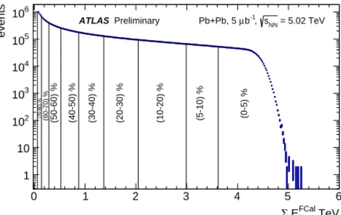
The minimum bias sample is divided into centrality classes. As the impact parameter is not measurable experimentally, the centrality selection is based on the strong monotonic correlation between the impact parameter and the transverse energy measured in the forward calorimeter,
ΣE
FCalT. The Glauber [24]
model is used to obtain the mapping from the observed
ΣE
TFCalto the elementary properties, such as the number of binary nucleon-nucleon interactions or the number of nucleons participating in the nuclear col- lision. The Glauber model provides also a correspondence between the
ΣE
FCalTdistribution and sampling fraction of the total inelastic Pb
+Pb cross section, allowing the setting of the centrality percentiles. For this analysis a selection of the 80% most central collisions (i.e. centrality (0–80)%) is used to avoid any biases from di
ffraction or other processes that contribute significantly to very peripheral collisions (cent- rality (80–100)%). Figure 1 shows the distribution of
ΣE
TFCalin data and thresholds for the selection of centrality intervals.
FCal TeV ET
Σ
0 1 2 3 4 5 6
events
1 10 102
103
104
105
106
Preliminary
ATLAS Pb+Pb, 5 µb-1, sNN = 5.02 TeV
(0-5) %
(5-10) %
(10-20) %
(20-30) %
(30-40) %
(40-50) %
(50-60) %
(60-70) %
(70-80) %
Figure 1: Distribution of the transverse energy in the FCal,EFCalT , for the min-bias event selection. The centrality bins are marked with vertical lines and labelled on the plot.
In order to study the performance of the ATLAS detector, a minimum-bias sample of 3
·10
5Pb-Pb MC events was generated using version 1.38b of HIJING [25]. The effect of flow is added after the generation using an “afterburner” [26] procedure in which the p
T,
ηand centrality dependence of the
vnas measured in the
√s
NN =2.76 TeV Pb
+Pb data is implemented. The generated sample is passed through a full simulation of the ATLAS detector using Geant 4 [27], and the MC events are reconstructed by the same reconstruction algorithms as the data.
4 Track Selection
The charged-particle tracks are reconstructed from the signals in the ID. A special reconstruction pro- cedure, optimized for tracking in dense environments, is used for this purpose [28]. In the analysis the set of reconstructed tracks is filtered using several selection criteria. The tracks are required to have p
T >0.5 GeV,
|η| <2.5, at least two pixel hits, with the additional requirement of a hit in the first pixel layer when one is expected
2, at least eight SCT hits, and at most one missing hit
3in the SCT. In addition, the transverse (d
0) and longitudinal (z
0sin(θ)) impact parameters of the track relative to the vertex are re- quired to be less than 1 mm. The track-fit quality parameter
χ2/ndof is required to be less than 6. Finally,in order to remove tracks with mismeasured p
Tdue to interactions with the material or other effects, the track-fit
χ2probability is required to be larger than 0.01 for tracks having p
T >10 GeV.
The MC sample is used to determine the track-reconstruction e
fficiency as a function of p
Tand
η,
(p
T, η).At mid-rapidity (|η|
<1) the reconstruction efficiency is
∼70% at lowp
Tand increases to
∼75% at higherp
T. For
|η| >1 the e
fficiency decreases to about (40–50)% depending on the p
T. The reconstruction e
fficiency depends weakly on the centrality for low p
Ttracks, for which it is smaller in the most central events by about 4% as compared to mid-central and peripheral collisions. For tracks with p
T >1 GeV the dependence on centrality is less than 1%. The fraction of tracks that are not associated with stable generated MC particles, but are produced from random combinations of hits in the ID (“fake tracks”), is found to vary significantly depending on
η. For|η| <1, it is
∼2% for low-pTtracks in the most central (centrality (0–5)%) Pb
+Pb events, and much below 1% for higher p
Tin more peripheral collisions. In the forward part of the detector, especially for 1
< |η| <2 where detector services reside, the fake rate is up to 8% at low p
Tand for the most central collisions. The fake rate drops rapidly for higher p
Tand also decreases gradually towards more peripheral collisions so that it is almost negligible already in the (20–30)% centrality interval.
5 Analysis Procedure
Two analysis techniques are used to determine the flow harmonics: the 2PC method, which uses only the information from the tracking detectors, and the SP method, which uses in addition the FCal. In both approaches the di
fferential flow harmonics are first obtained in narrow intervals of p
T,
ηand centrality.
Integrated quantities are obtained by taking into account the track reconstruction efficiency,
, and fakerate, f . A p
T-,
η- and centrality-dependent weight factorw=(1
−f )/ is applied to each track in the 2PC measurement and to scale each bin of the di
fferential
vndistributions in the SP method.
2A hit is expected if the extrapolated track crosses an active region of a pixel module that has not been disabled.
3 A hit is said to be missing when it is expected but not found.
5.1 Two particle correlation analysis
The 2PC method has been used extensively by ATLAS for correlation measurements [10, 29–33]. In the 2PC method, the distribution of particle pairs in relative azimuthal angle
∆φ=φa−φband pseudorapidity separation
∆η = ηa−ηbis measured. Here the labels a and b denote the two particles used to make the pair. They are conventionally called the “trigger” and “associated” particles, respectively. The two particles involved in the correlation measurement can be selected using various criteria, for example different p
Tranges (hard-soft correlations), different rapidity (forward-backward correlation), different charge combination (same-sign or opposite-sign correlation) or different particle species etc. In this analysis, the two particles are charged hadrons measured by the ATLAS tracking system, over the full azimuth and
|η|<2.5, resulting in a pair-acceptance coverage of
±5.0 units in
∆η.In order to account for the detector acceptance e
ffects, the correlation is constructed from the ratio of the distribution in which the trigger and associated particles are taken from the same event to the dis- tribution in which the trigger and associated particles are taken from two different events. These two distributions are referred to as the “same-event” (S) or “foreground” distribution and the “mixed-event”
or “background” (B) distribution, respectively, and the ratio is written as:
C(
∆η,∆φ)=S (
∆φ,∆η)B(
∆φ,∆η).(2)
The same-event distribution includes both the physical correlations and correlations arising from detector acceptance e
ffects. On the other hand, the mixed-event distribution reflects only the e
ffects of detector ine
fficiencies and non-uniformity, but contains no physical correlations, To ensure that the acceptance effects in the B distribution match closely in the S distribution, the B distribution is constructed from particles from two di
fferent events that have similar multiplicity and z-vertex. Furthermore, in order to account for the e
ffects of tracking e
fficiency
(p
T, η), each pair is weighted by (pa 1T,ηa)(pbT,ηb)
for S and B.
In the ratio C, the acceptance effects largely cancel out and only the physical correlations remain [34].
Typically, the two-particle correlations are used only to study the shape of the correlations in
∆φ, and areconveniently normalised. In this note, the normalisation of C(∆
η,∆φ) is chosen such that the∆φ-averagedvalue of C(∆
η,∆φ) is unity for|∆η|>2.
Figure 2 shows C(
∆η,∆φ) for several centrality intervals for 2<p
a,bT <3 GeV, where p
aTand p
bTlabel the p
Tof the trigger and associated particles used in the correlation. In all cases a peak is seen in the correlation at (
∆η,∆φ) ∼(0, 0). This peak arises from short-range correlations such as decays, Hanbury Brown and Twiss (HBT) correlations [35], or jet-fragmentation. The long-range (large
∆η) correlations are the resultof the global anisotropy of the event and are the focus of the study in this note.
To investigate the
∆φdependence of the long-range (
|∆η|>2) correlation in more detail, the projection on to the
∆φaxis is constructed as follows:
C(
∆φ)= R52
d|
∆η|S (
∆φ,|∆η|) R52
d|
∆η|B(
∆φ,|∆η|) ≡S (
∆φ)B(
∆φ).(3)
The
|∆η|>2 requirement is imposed to reject the near-side jet peak and focus on the long-range features
of the correlation functions.
∆φ 0 2 4
∆η -4 -2 0 2 4
)φ∆,η∆C(
0.98 1 1.02 1.04
ATLASPreliminary b-1
µ
=5.02 TeV, 22 sNN
Pb+Pb
<3 GeV
b , a
pT
2<
(0-5)%
∆φ 0 2 4
∆η -4 -2 0 2 4
)φ∆,η∆C(
0.9 1 1.1
ATLASPreliminary b-1
µ
=5.02 TeV, 22 sNN
Pb+Pb
<3 GeV
b , a
pT
2<
(25-30)%
∆φ 0 2 4
∆η -4 -2 0 2 4
)φ∆,η∆
C( 0.91 1.1 1.2
ATLASPreliminary b-1
µ
=5.02 TeV, 22 sNN
Pb+Pb
<3 GeV
b , a
pT
2<
(55-60)%
Figure 2: Two-particle correlation functionsC(∆η,∆φ) in 5.02 TeV Pb+Pb collisions for 2<pa,bT <3 GeV. The left middle and right panels correspond to the (0–5)%, (25–30)% and (55–60)% centrality classes respectively.
In a similar fashion to the single-particle distribution Eq.(1), the 2PC can be expanded as a Fourier series:
C(∆
φ)=C
01
+ Σ∞n=1vn,n( p
aT,p
bT) cos(n
∆φ).
(4)
If the two-particle distribution is simply the product of two single-particle distributions, then it can be shown that the Fourier coe
fficients of the 2PC factorize as:
vn,n
(p
aT,p
bT)
=vn( p
aT)v
n( p
bT) (5) The factorization of
vn,ngiven by Eq. (5) is expected to break at high p
Twhere the anisotropy does not arise from flow. The factorization is also expected to break when the
ηseparation between the particles is small, and short-range correlations dominate. However, the
|∆η|>2 requirement removes most of such short-range correlations. In the phase-space region where Eq. (5) holds, the
vn( p
bT) can be evaluated from the measured
vn,nas:
vn
( p
bT)
= vn,n( p
aT,p
bT)
vn
(p
aT)
= vn,n( p
aT,p
bT)
pvn,n
(p
aT,p
aT)
,(6) where in the denominator, the condition
vn,n(p
aT,p
aT)
= v2n( p
aT) is used. In this analysis, for most of the 2PC results the
vn( p
bT) will be evaluated using Eq (6) with 0.5< p
aT<5.0 GeV. The lower cutoffof 0.5 GeV on p
aTcomes from the range over which the measurements are done in this note (0.5–25 GeV). The upper cuto
ffon p
aTis chosen to exclude high- p
Tparticles which predominantly come from jets and are not expected to obey Eq. (6).
Figure 3 shows one-dimensional 2PCs as a function of
∆φfor 2
<p
a,bT <3 GeV and for several di
fferent centrality intervals. The correlations have been normalized to have a mean value (C
0in Eq. (4)) of 1.0.
The continuous line is a Fourier fit to the correlation (Eq. (4)) that includes harmonics up to n
=6. Thecontribution of the individual
vn,nare also shown. The modulation in the correlation about its mean
value is the smallest in the most central events (top left panel) and increases towards mid-central events
reaching a maximum in the (45–50)% centrality interval and then decreases. In central collisions, the
v2,2-v
4,4are of comparable magnitude. But for other centralities, where the average collision geometry
is elongated, the
v2,2is significantly larger than the other
vn,nfor n
≥3. In the central events the away-
side peak is also much broader because all the significant harmonics are of similar magnitude, while in
mid-central events the near and away-side peaks are quite symmetric as the
v2,2dominates. In central
and mid-central events, the near-side peak is larger than the away-side peak. However, for centralities
(60-80)% the away-side peak becomes larger due to the presence of a large negative
v1,1component. This negative
v1,1component in the peripheral 2PCs arises largely from dijets: while the near-side jet peak is rejected by the
|∆η|>2 cut, the away-side jet position varies in
|∆η|from event to event, and cannot be rejected entirely. In the peripheral multiplicity intervals, the away-side jet significantly a
ffects the 2PC.
It produces a large negative
v1,1and also affects the other harmonics by adding alternatingly positive and negative contributions to them: i.e. positive contribution to
v2,2, negative contribution to
v3,3, positive contribution to
v4,4and so on. In peripheral events the
vn,nare strongly biased by dijets especially at higher p
T. The presence of the jets also results in the breakdown of the factorization relation (Eq. (6)).
5.2 Scalar Product and Event Plane analysis
The SP method has been introduced by the STAR collaboration [36] and is further discussed in Ref.
[13]. The SP method is very similar to the Event Plane method (EP) widely used in earlier analyses [9, 10]. It is superior to the EP as
vn{SP
}is an estimator of
phv2ni
, independent of the detector resolution and acceptance, whereas
vn{EP}produces a detector-dependent estimate of
vnthat lies between
hvniand
phv2ni[5, 37].
The SP method uses flow vectors defined as Q
n=|Qn|einΨn =1
S
Xj=1,S
q
n,j=1 S
X
j=1,S
wj
e
inφj,(7)
where the sum runs over S particles in a single event, restricted to a selected region of phase space of (η, p
T). The
φjis the particle azimuthal angle and n is the harmonic order. In this analysis the flow vectors are established separately for the two sides of the FCal and are denoted Q
N|Pn, where the N and P correspond to the two sides of the detector (N for
η <0 and P for
η >0). The sum in Eq. (7) in this case runs over the calorimeter towers of approximate granularity
η×φ=0.1
×0.1 and the weights
wiare linear functions of the E
Tof the towers. The tower E
Tis scaled so that the response, averaged over all events in the data-taking run, is identical for each tower in the
ηslice. A similar “flattening” procedure is applied when Q
nis calculated using charged-particle tracks. In this case the weight
wjis the inverse of the relative track-reconstruction e
fficiency, which is obtained from the data as the inverse of the track multiplicity in the narrow
η×φ=0.1
×0.1 interval, normalised such that the average e
fficiency in one
ηslice of 0.1 width is unity.
The values of
vnin this analysis are obtained as
vn,j{SP}=Re
hqn,jQ
nN|P∗iphQNn
Q
P∗n i = h|qn,j||QN|Pn |cos[n(φj−ΨnN|P)]
i ph|QnN||QPn|cos[n(ΨNn −ΨPn)]i
,
(8)
where q
n,jis the flow vector obtained for a small (η, p
T) interval (typically 0.1 in
ηand in p
T0.1 GeV at low p
Tand 1 GeV at higher p
T) using tracks, Q
nN|Pis the flow vector obtained using either the N or P side of the FCal, chosen so that the
ηgap between the
ηof the q
n,jinterval and Q
nis maximised, the * denotes complex conjugation, the
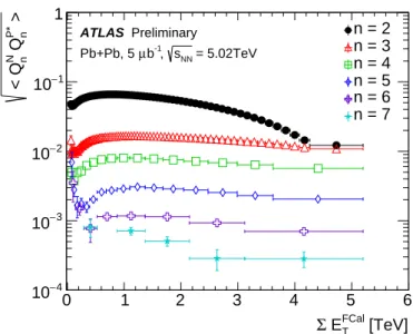
Ψnare estimates of the n-th order reacion-plane angles (Eq. (7)) and the angular brackets indicate an average over all events. In the rightmost expression in Eq.(8) it is assumed that the sine terms disappear. The inverse of the correction factor,
phQnN
Q
nP∗i, (denominator in Eq. (8)) dependson the harmonic order and
ΣE
FCalTas shown in Fig. 4.
φ
∆
0 2 4
)φ∆C(
1 1.02
ATLAS Preliminary b-1
=5.02 TeV, 22 µ sNN
Pb+Pb
(0-5)% 2<|∆η|<5
<3 GeV b , a pT 2<
φ
∆
0 2 4
)φ∆C(
0.98 1 1.02 1.04
1.06 ATLAS Preliminary b-1
=5.02 TeV, 22 µ sNN
Pb+Pb
(5-10)% 2<|∆η|<5
<3 GeV b , a pT 2<
φ
∆
0 2 4
)φ∆C(
1 1.05
ATLAS Preliminary b-1
=5.02 TeV, 22 µ sNN
Pb+Pb
(10-15)% 2<|∆η|<5
<3 GeV b , a pT 2<
φ
∆
0 2 4
)φ∆C(
0.95 1 1.05 1.1
ATLAS Preliminary b-1
=5.02 TeV, 22 µ sNN
Pb+Pb
(15-20)% 2<|∆η|<5
<3 GeV ,b a pT 2<
φ
∆
0 2 4
)φ∆C(
0.95 1 1.05 1.1
1.15 ATLAS Preliminary b-1
=5.02 TeV, 22 µ sNN
Pb+Pb
(20-25)% 2<|∆η|<5
<3 GeV ,b a pT 2<
φ
∆
0 2 4
)φ∆C(
1 1.1
ATLAS Preliminary b-1
=5.02 TeV, 22 µ sNN
Pb+Pb
(25-30)% 2<|∆η|<5
<3 GeV ,b a pT 2<
φ
∆
0 2 4
)φ∆C(
0.9 1 1.1
ATLAS Preliminary b-1
=5.02 TeV, 22 µ sNN
Pb+Pb
(30-35)% 2<|∆η|<5
<3 GeV b , a T 2<p
φ
∆
0 2 4
)φ∆C(
0.9 1 1.1
1.2 ATLAS Preliminary b-1
=5.02 TeV, 22 µ sNN
Pb+Pb
(35-40)% 2<|∆η|<5
<3 GeV b , a T 2<p
φ
∆
0 2 4
)φ∆C(
0.9 1 1.1
1.2 ATLAS Preliminary b-1
=5.02 TeV, 22 µ sNN
Pb+Pb
(40-45)% 2<|∆η|<5
<3 GeV b , a T 2<p
φ
∆
0 2 4
)φ∆C(
0.9 1 1.1
1.2 ATLAS Preliminary b-1
=5.02 TeV, 22 µ sNN
Pb+Pb
(45-50)% 2<|∆η|<5
<3 GeV b , a pT 2<
φ
∆
0 2 4
)φ∆C(
0.9 1 1.1
ATLAS Preliminary b-1
=5.02 TeV, 22 µ sNN
Pb+Pb
(50-55)% 2<|∆η|<5
<3 GeV b , a pT 2<
φ
∆
0 2 4
)φ∆C(
0.9 1 1.1
ATLAS Preliminary b-1
=5.02 TeV, 22 µ sNN
Pb+Pb
(55-60)% 2<|∆η|<5
<3 GeV b , a pT 2<
φ
∆
0 2 4
)φ∆C(
0.95 1 1.05 1.1
ATLAS Preliminary b-1
=5.02 TeV, 22 µ sNN
Pb+Pb
(60-65)% 2<|∆η|<5
<3 GeV b , a pT 2<
φ
∆
0 2 4
)φ∆C(
0.95 1 1.05 1.1
ATLAS Preliminary b-1
=5.02 TeV, 22 µ sNN
Pb+Pb
(65-70)% 2<|∆η|<5
<3 GeV b , a pT 2<
φ
∆
0 2 4
)φ∆C(
0.95 1 1.05 1.1
ATLAS Preliminary b-1
=5.02 TeV, 22 µ sNN
Pb+Pb
(70-75)% 2<|∆η|<5
<3 GeV b , a pT 2<
Figure 3: One dimensional two-particle correlation functions C(∆φ) in 5.02 TeV Pb+Pb collisions for 2<pa,bT
<3 GeV(points). The solid-black line indicates a fit to Eq. (4) containing harmonicsvn,n up ton=6. The dashed grey line shows the contribution of thev1,1. The contributions of thev2,2–v6,6 are indicated by the coloured lines (v2,2- red,v3,3- blue,v4,4- magenta,v5,5-orange,v6,6- green). Each panel corresponds to a different centrality class.
They-axis range for the different panels is different.
[TeV]
FCal
ET
Σ
0 1 2 3 4 5 6
>P* n QN n < Q
−4
10
−3
10
−2
10
−1
10 1
Preliminary ATLAS
= 5.02TeV sNN
-1, µb Pb+Pb, 5
n = 2 n = 3 n = 4 n = 5 n = 6 n = 7
Figure 4: The dependence of the correction factor in the SP method, q
hQNnQP∗n i, for all measured harmonics as a function ofΣEFCalT binned according to the centrality bins definition.
In the Event Plane analysis the reference Q vectors are normalised to unity, Q
N|Pn →Q
N|Pn /|QnN|P|, before using them in Eq. (8). So the
vnestimate is obtained as
vn{EP}=
Re
D
q
n,jQN|P∗n|QnN|P|
E r
DQN n
|QNn| QnP∗
|QPn|
E
= hcos[n(φj−ΨN|Pn
)]i
phcos[n(ΨNn −ΨPn)]i
.
(9)
In this analysis the EP method is used only for the purpose of a direct comparison with the results obtained in Run 1, in which the EP method was used.
The analysis is performed in intervals of centrality. The
vnvalues are obtained in narrow bins of p
Tand
η, which are summed, taking into account tracking efficiency and fake rate, to obtain the integrated results.
6 Systematic Uncertainties
The systematic uncertainties of the measured
vnare evaluated by varying several aspects of the analysis.
The uncertainties of the EP results are very similar to those for the SP results, and are not discussed separately. Similarly, some of the uncertainties are common in their origin between the EP
/SP and the 2PC methods and are discussed together. The uncertainties are summarised in the Table 1 and 2 for the 2PC and SP/EP methods respectively. The following sources of uncertainties are considered:
• Track selection:
The tracking selection cuts control the relative contribution of genuine charged
particles and fake tracks entering the analysis. The stability of the results to the track selection
is evaluated by varying the requirements imposed on the reconstructed tracks. For each variation,
the entire analysis is repeated including the evaluation of the corresponding efficiencies and fake
rates. At the low p
Tthe variation in the
vnobtained from this procedure is most significant in the most central events, as the fake rate is largest in this region of phase space, and typically of the order of 5%. For higher p
T, changing the set of tracks used in the analysis has less influence on the measurement.
• Tracking efficiency:
As mentioned above, the tracks are weighted by 1/(p
T, η) when calculatingthe
vnto account for the e
ffects of the tracking e
fficiency. Uncertainties in the e
fficiency, resulting e.g. from an uncertainty of the detector material budget, need to be propagated into the measured
vn. This uncertainty is evaluated by varying the efficiency up and down within its uncertainties in a p
Tdependent manner and re-evaluating the
vn. This contribution to the overall uncertainty is very small and amounts to less than 1% on average. This is because the change of efficiency cancels out in the differential
vn( p
T) measurement, and for
vnintegrated over p
T, the low- p
Tparticles dominate the measurement. It does not change significantly with centrality nor with the order of harmonics.
• Uncertainty in the centrality determination:
A scale uncertainty on the flow harmonics comes from the uncertainty in the fraction of the total inelastic cross-section accepted by the trigger and the event selection criteria. It is evaluated by varying the centrality bin definitions, using the modified selections, which account for the 1% uncertainty in the sampled fraction of the cross-section. The changes in the
vnare largest in the peripheral-centrality intervals, for which the bin definitions are significantly changed when remapping the centralities. For
v2, a change of
∼0.8% (2PC) and∼
1.5% (SP) is also observed in the most central events. This is because the
v2changes rapidly with centrality in central events, so slight variations in the centrality definition result in significant change in
v2. For
v3this uncertainty varies from less than 0.5% over the (0–50)% centrality range to
∼5% in the (70–80)% centrality. For the higher-order harmonics n
>3 the uncertainty is less than 0.5% over the (0–50)% centrality range and increases to about 2% for more peripheral bins.
The variation in the
vnwhen using these alternative centrality definitions is taken as a systematic uncertainty. Significant changes in the sample of events in the peripheral bins affect the
v7at high p
T, indicating statistical instability of this measurement.
• MC Closure:
The MC closure test consists of comparing the
vtruenobtained directly from the MC generated particles, and the
vreconobtained by applying the same procedures to the MC sample as are applied to the data. The analysis of MC events is done to evaluate the contributions of e
ffects not corrected for in the data analysis. The two-particle correlation analysis is validated by measuring the
vn,nof reconstructed particles in fully simulated HIJING events and comparing them to those obtained using the generated particles. For the SP method the Q
N|Pnvectors are obtained with generated particles falling into the acceptance of the FCal (3.2
< η <4.8). Due to the limited size of the MC sample, this contribution cannot be established for small
vnsignals of high-order harmonics:
v6and
v7, and
v4and
v5in more peripheral collisions. This uncertainty is at the level of a few percent, where the statistics permits a sensible estimate.
• ηasymmetry:
Due to the symmetry of the Pb+Pb collision system the event-averaged
hvn(η)i and
hvn(−η)i are expected to be equal. Any di
fference between the event-averaged
vnat
±ηarises from residual detector non-uniformity. The di
fference between the
vnvalues measured in opposite hemi- spheres is treated as the systematic uncertainty quantifying a non-perfect detector performance.
This uncertainty is in general very low (at the level of 1%) except for high-order harmonics
v5and
v6at high p
Tand
v7at all p
T. This uncertainty only contributes to the
vnvalues measured by the
EP and SP methods. For the 2PC method, the residual non-uniformity is estimated by variation in
the event-mixing procedure.
• Residual sine term:
The ability of the detector to measure small
vnsignals can be quantified by comparing the value of the
vncalculated as the real part of the flow vector product (SP) in Eq (8) to its imaginary part. The ratio Im(S P)/v
nis taken as a contribution to the systematic uncertainty.
As the values of Im(S P) as well as the
vnare small, the limited numerical precision causes the ratio to vary significantly in bins of lower statistics. Therefore a common uncertainty for all tracks of p
T >1.5GeV is obtained and propagated to p
Tbins above 1.5 GeV. The contribution from this source is
∼1% in most of the phase space, while for the higher harmonics (n=5, 6) and for the low p
T(0.5
−0.6 GeV) it can reach 45% in the most central collisions. This uncertainty is only relevant for the
vnvalues measured by the EP and SP methods.
• Variation of FCal acceptance inQN|Pn estimation:
In order to quantify an uncertainty arising from FCal acceptance in Q
nN|Pestimation,
vnharmonics are compared for two distinct FCal regions 3.2
< |η| <4 and 4
< |η| <4.8 used for the determination of the reference flow vector, Q
n. The di
fferences in the
vn’s are treated as the systematic uncertainty, which, similarly to the
ηsymmetry, quantifies the ability of the detector to measure small signals. Accordingly, this contribution is small (of the order of about 1% ) for
v2and
v3and starts growing for higher order harmonics up to about 80% for
v7. This uncertainty is only relevant to the
vnvalues measured by the EP and SP methods.
• Event-mixing
As explained in Section 5.1, the 2PC analysis uses the event-mixing technique to
estimate and correct for the detector acceptance effects. Potential systematic uncertainties in the
vndue to the residual pair-acceptance effects, which were not corrected by the mixed events, are
evaluated following Ref. [10]. The resulting uncertainty on the
v2–v
5is between 1–3%, and for
v6is between 4–8% for most of the centrality and p
Tranges measured in this note. However,
the uncertainties for
v4–v
6are significantly larger for p
T<0.7 GeV where the
vnsignals are quite
small and very susceptible to acceptance e
ffects. The uncertainties are also significantly larger for
p
T>10 GeV where they are correlated with statistical uncertainties.
systematic
sources n harmonic 5 - 10 % 50 - 60 %
0.5–0.6 GeV 6–8 GeV 0.5–0.6 GeV 6–8 GeV
tracking cuts
v2
8 3 1 1
v3
8 3 1 2
v4
11 4 3 4
v5
16 5 4 5
v6
16 8 4 8
efficiency variation
v2
0.2
<0.10.2
<0.1v3
0.2 0.2 0.3 0.7
v4
0.3 0.2 0.3 0.7
v5
0.2
<0.10.2 1.0
v6
4.8 11 4.2 0.9
centrality
v2
1 1 1.5
<0.5
v3
0.5 0.5 3 10
v4
0.5 0.5 3 10
v5
0.5 0.5 3 10
v6
0.5 0.5 3 10
MC closure
v2
6 3 3 1
v3
6 3 3 1
v4
5 5 5 5
v5
6 6 6 6
v6
10 10 10 10
event- mixing
v2
1 1 1 1
v3
1 2 1 4
v4
5 6 3 6
v5
5 10 5 10
v6
50 15 50 15
Table 1: The systematic uncertainties associated with the 2PCvn measurements for selected intervals of pT and centrality. The contributions are experessed in %.
systematic
sources n harmonic 5 - 10 % 50 - 60 %
0.5 - 0.6 GeV 9 - 10 GeV 0.5 - 0.6 GeV 9 - 10 GeV
tracking cuts
v2
5 (5) 0.2 (0.3) 0.1 (0.1) 0.3 (0.3)
v3
6 (6) 0.2 (0.2) 0.2 (0.1) 3 (2)
v4
6 (6) 0.4 (0.2) 3 (3) 1 (3)
v5
7 (9) 0.2 (1) 2 (2) 3 (2)
v6
14 (17) 1 (3) 3 (6) 3 (6)
v7
2 (12) 9 (3) 6 (26) 6 (26)
e
fficiency variation
v2
0.2 (0.2)
<0.1 (<0.1)0.2 (0.2)
<0.1 (<0.1) v30.2 (0.2) 0.2 (<0.1) 0.3 (0.3) 0.7 (0.5)
v40.3 (0.3) 0.2 (0.3) 0.3 (0.2) 0.7 (0.5)
v50.2 (0.2)
<0.1 (0.2)0.2 (0.2) 1 (3)
v6
5 (17) 11 (2) 5 (6) 0.9 (2)
v7
3 (3) 0.1 (0.4) 2 (4) 2 (2)
η
symmetry
v2
0.8 (0.7)
<0.1 (
<0.1) 0.2 (0.1) 0.3 (
<0.1)
v3
1 (1) 0.5 (0.3) 0.6 (0.5) 1 (0.5)
v4
1 (1) 0.4 (0.9) 2 (5) 4 (9)
v5
2 (2) 3 (5) 4 (4) 3 (3)
v6
10 (7) 4 (4) 11 (7) 11 (7)
v7
11 (15) 11 (15) 15 (12)
centrality
v2
1 (1) 1 (1) 0.5 (0.3) 1 (1)
v3
0.2 (0.2) 0.2 (
<0.1) 0.3 (0.3) 0.7 (0.5)
v4 <0.1 (
<0.1) 0.4 (0.7) 1 (3) 0.8 (3)
v5
2 (2) 0.2 (0.5) 4 (4) 2 (1)
v6
2 (1) 2 (2) 2 (3) 2 (3)
v7
11 (7) 8 (7) 4 (4) 4 (4)
residual sine term
v2
0.2 (0.2) 0.1 (
<0.1) 0.4 (0.5) 0.3 (0.5)
v3
0.5 (0.5) 1 (1) 2 (2) 1 (0.4)
v4
1 (2) 0.7 (1) 0.2 (3) 6 (4)
v5
3 (4) 0.1 (3) 11 (13) 11 (4)
v6
3 (11) 17 (21) 21 (31) 21 (31)
v7
34 (26) 35 (43)
MC closure
v2
2 (2) 1 (1) 0.3 (<0.1) 1 (1)
v3
2 (3) 2 (1) 14 (14) 11 (11)
40-50%
v4
4 (4) 0.5 (1) 1 (3) 5 (9)
10-20%
v5
3 (7) 14 (21) 8 (7) 2 (3)
v6
- - - -
v7
- - - -
residual FCal mis- calibration
v2
0.1 (0.4) 0.7 (1) 0.1 (
<0.1) 2 (0.6)
v3
1 (2) 2 (2) 0.3 (2) 8 (10)
v4
2 (3) 4 (6) 3 (2) 0.1 (6)
v5
8 (6)
<0.1 (4)5 (8) 2 (3)
v6
17 (5) 5 (17) 28 (3) 28 (3)
v7
34 (13) 34 (13) 34 (13) 34 (13)
7 Results
7.1 p
Tdependence
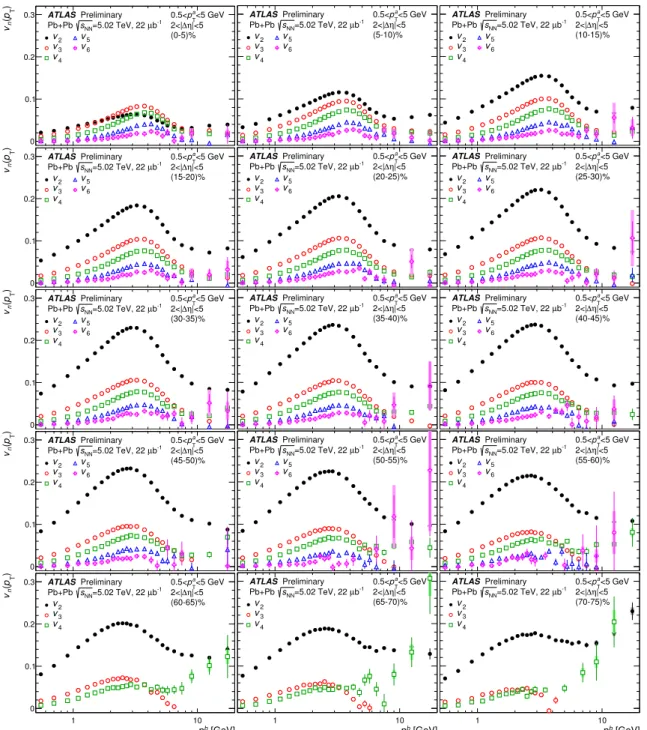
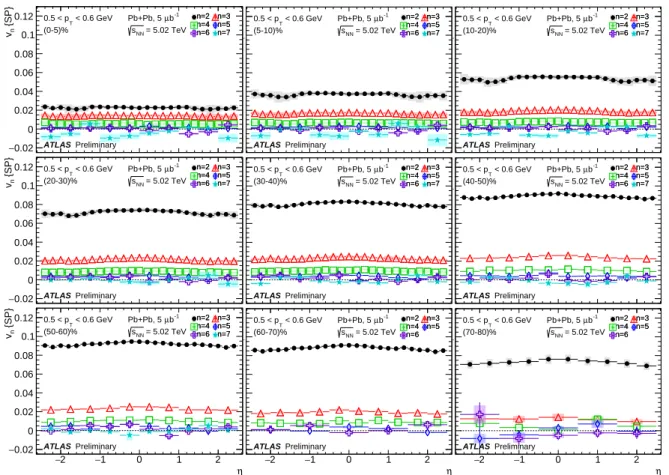
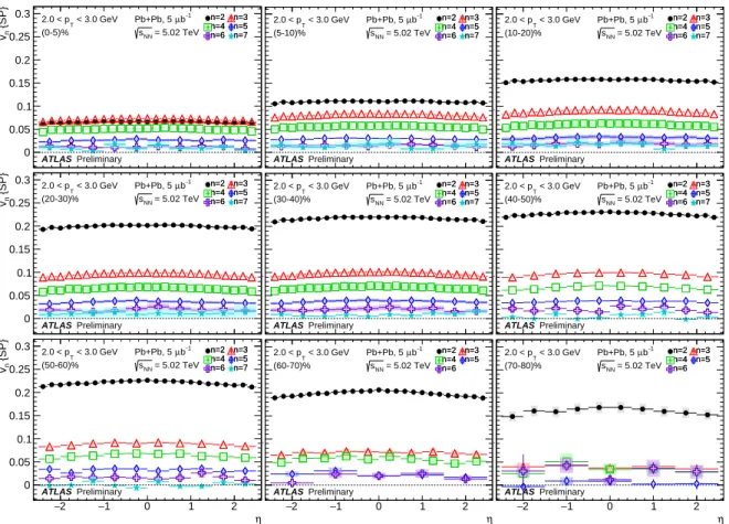
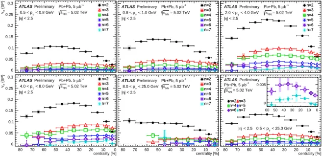
Figures 5 and 6 show the
vnobtained from the SP and 2PC methods, respectively, as a function of p
Tfor several centrality intervals. The SP results are integrated over the pseudorapidity
|η| <2.5. The 2PC results are obtained with 0.5< p
aT <5 GeV and for|∆η|>2. Thevnvalues show a similar p
Tdependence across all centralities: a nearly linear rise to about 2 GeV, followed by a gradual increase to reach a maximum around 2.5-3.5 GeV and a gradual fall at higher p
T. However, significant
vnvalues persist even at the highest measured p
T(
∼20 GeV), especially for
v2. In peripheral events, at the highest p
T, the 2PC-v
2values again show an increasing trend due to the increasing influence of the away-side jet. The increased
v2is accompanied by reduced values of
v3and increased values of
v4, which is characteristic of a large away-side peak, as described in Section 5.1. This is most clearly seen in the (70–75)% centrality interval, where the 2PC
v2values show a strong increase beyond p
T∼10 GeV. The
v2varies significantly with centrality, reflecting a change in the shape of the average initial collision geometry, from nearly circular in central collisions to an almond shape in peripheral events. The higher harmonics do not show similar behaviour, as neither higher-order eccentricities nor the fluctuations vary so significantly with the centrality. The
v2is dominant at all centralities, except in the (0–5)% interval where at high p
T v3and
v4become larger than
v2, indicating that the dominant source of observed flow comes from the initial geometry fluctuations. The
v4, similarly to
v2, exhibits an increase beyond p
T ∼10GeV, which can be attributed to the presence of the events with di-jets in the data. In the SP measurement the
v7results are also presented. The characteristics of
v7are similar to the other high-order harmonics, but the values are smaller and significant, given the uncertainties, only in central and mid-central collisions and for the p
Trange of 2.5–3.5 GeV.
Figure 7 compares the
vnvalues measured with the EP and SP methods for the integrated p
Trange of 0.5< p
T <25 GeV. A small difference is seen between the v2values measured with the two methods.
The di
fference is largest in mid-central events: about 3% in the (20–30)% centrality interval, about 1%
in the (0–5)% most central collisions and negligible in peripheral collisions. This difference is expected according to [37] as the SP method measures
phv2ni
while the EP method measures a value in between
hvniand
phv2ni, with the former value attained in the limit of the correction factor (the inverse of the
denominator in Eq. (9)) approaching unity and the latter when it is large. In the most central and peripheral events, where the correction is large for the second-order harmonic, the EP
v2values are closer to the SP ones, while for the mid-central events where the correction is small, the EP
v2values are systematically lower than the SP
v2values. For higher-order harmonics, the difference between the EP and SP
vnvalues is consistent with zero, which implies that the EP measurements are always in the limit of large correction factor.
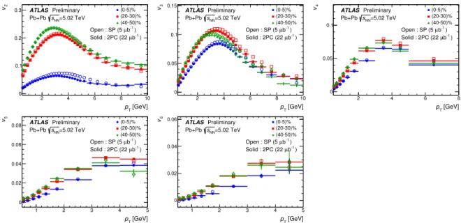
Figure 8 shows a comparison of the SP and 2PC results. There is significant difference between the
v2values measured by the two methods in the (0–5)% centrality intervals, with the SP method giving con- sistently higher values. This difference decreases considerably for (20–30)% mid-central events, where the
v2values match within 2–5% up to p
T ∼10 GeV. A roughly similar trend is observed in the higher- order harmonics, where the di
fference between the 2PC and SP
vnvalues is largest in the most central events, and decreases for mid-central events. For
v3and
v4, where statistics allow for a clear comparison, the
vnvalues match within
∼5% forp
T <4 GeV for the three centrality intervals shown in Figure 8. In principle both the SP and 2PC methods measure
phv2ni