Measurement of multi-particle azimuthal correlations with the subevent cumulant method in pp and p+Pb collisions with the ATLAS detector

A TLAS-CONF-2017-002 08 Febr uary 2017

ATLAS CONF Note

ATLAS-CONF-2017-002

Measurement of multi-particle azimuthal

correlations with the subevent cumulant method in pp and p + Pb collisions with the ATLAS detector

The ATLAS Collaboration

1st February 2017

The measurement of four-particle cumulant elliptic flow coefficients c

{ 4 } and v

{ 4 } are presented using 0.17 pb

of pp data at √

s = 5.02 TeV, 0.9 pb

of pp data at √ s = 13 TeV and 28 nb

of p + Pb data at √ s

= 5.02 TeV. The values of c

{ 4 } are calculated as a function of average number of charged particles, ⟨ N

⟩ , using the standard cumulant method and recently proposed two-subevent and three-subevent methods. The three-subevent method is found to be less sensitive to short-range correlations, originating mostly from jets. The three-subevent method gives a negative c

{ 4 } , and thus a well-defined v

{ 4 } = (− c

{ 4 })

, in these collision systems. The magnitude of the c

{ 4 } is found to be nearly independent of ⟨ N

⟩ . Furthermore, v

{ 4 } is found to be smaller than the v

{ 2 } measured using the two- particle correlation method, as expected for a long-range collective behaviour. Following a recent model framework, the measured values of v

{ 4 } and v

{ 2 } are used to probe the number of sources in the initial state collision geometry.

© 2017 CERN for the benefit of the ATLAS Collaboration.

Reproduction of this article or parts of it is allowed as specified in the CC-BY-4.0 license.

1 Introduction

The study of azimuthal correlations in high energy nuclear collisions at the RHIC and LHC has been an important avenue for understanding the multi-parton dynamics of QCD in the strongly-coupled non- perturbative region. One striking observation is the long-range ridge [1–5] in two-particle angular cor- relations (2PC): an apparent collimated emission of particle pairs with small relative azimuthal angle ∆ φ and large separation in pseudorapidity ( ∆ η). The ridge signal from 2PC is characterized by a Fourier de- composition ∼ 1 + 2v

cos ( n ∆ φ ) , where v

denotes the single-particle anisotropy harmonics. The second- order coefficient v

is by far the largest, followed by v

. The ridge was first discovered in nucleus–nucleus (A + A) collisions [1–6], but was later observed in proton–nucleus (p + A) and light-ion–nucleus colli- sions [7–12], and more recently also observed in high multiplicity proton-proton ( pp) collisions [13–16].

The ridge in large systems such as central or mid-central A+A collisions, is commonly interpreted as the result of collective hydrodynamic expansion of hot and dense nuclear matter created in the overlap region.

Since the formation of an extended nuclear matter is not necessarily expected in small collision systems such as p +A and pp, the origin of the ridge could be different from that in large collision systems. There remains a considerable debate in the theoretical community on whether the ridge in small systems is of hydrodynamic origin similar to A + A collisions [17] or is induced by gluon saturation in the initial state of the colliding particles [18].

From the experimental perspective, a central question about the ridge is whether it involves all particles in the event (collective flow) or if it arises merely from correlations among a few particles, due to res- onance decays, minijets, or multi-jet production (non-flow). In small systems, the contributions from non-flow sources, in particular jets and dijets, are very large. The extraction of ridge signal using the 2PC method requires large η gap and a careful removal of a large contribution from dijets. The lat- ter is estimated from 2PC in very low multiplicity events and then subtracted from higher multiplicity events [8, 9, 11, 14, 15, 19]. Since collectivity is intrinsically a multi-particle phenomenon, it can be probed more directly using multi-particle correlation techniques, known as multi-particle cumulants [20].

Azimuthal correlations involving four-, six-, eight-particles have been applied to p +Pb and pp collisions, and a finite v

signal has been obtained [12,19,21]. Although the standard multi-particle cumulant method reduces the non-flow correlations, it is important to study how e ff ective the suppression of non-flow is in this method. The v

extracted from four-particle cumulants c

{ 4 } , requires a negative c

{ 4 } value (see Sec. 2). However in pp and p + Pb collisions, the measured c

{ 4 } is observed to change sign at smaller values of the charged particle multiplicity [12, 16, 19, 21], N

. Furthermore the magnitude of c

{ 4 } and the N

value where sign change occurs are found to also depend on the exact definition of N

used to categorize the events as a function of multiplicity. Recently, an improved cumulant method based on the correlation between particles from di ff erent subevents separated in η has been proposed to further reduce the non-flow correlations [22]. The performance of this method for suppressing non-flow correlations has been validated using P ythia 8 event generator that contains only non-flow correlations, and no long-range collective particle emission.

This note presents the measurement of v

in pp collisions at √

s = 5.02 and 13 TeV, as well as p +Pb

collisions at √ s

= 5.02 TeV. The v

is obtained using two- and three-subevent cumulant methods and

is compared with the standard cumulant method. The results are compared with those obtained using a

two-particle correlation method in Refs. [11, 15] to assess the nature of the event-by-event fluctuation of

the collective flow in these collisions.

2 Four-particle cumulants

The multi-particle cumulant method [20] has the advantage of directly reducing correlations from jets and dijets, instead of relying on an explicit procedure to correct v

harmonics extracted in a 2PC approach for dijet correlations, as is done in Refs. [11, 14]. The mathematical framework for standard cumulant is based on the Q-cumulants discussed in Refs. [23, 24], which have been recently extended to the case of subevent cumulants in Ref. [22]. These methods are briefly summarized below.

The cumulant method involves the calculation of 2k-particle azimuthal correlations ⟨{ 2k }

⟩ , and cumu- lants, c

{ 2k } , for the n

-order flow harmonics. The two- or four-particle azimuthal correlations in one event are evaluated as [22–24]:

⟨{ 2 }

⟩ = ⟨ e

⟩ = q

− δ

1 − δ

(1)

⟨{ 4 }

⟩ = ⟨ e

⟩ = q

− 2δ

( Re [ q

q

] + 2q

) + 8δ

Re [ q

q

] + δ

( 2 + q

) − 6δ

1 − 6δ

+ 8δ

+ 3δ

− 6δ

,(2) where “ ⟨⟩ ” denotes average of all unique pairs or all unique quadruplets for two- or four-particle correla- tions, respectively. In Eqs. 1 and 2, these averages have been expanded into per-particle normalized flow vector q

and factors δ

with l = 1, 2...:

q

≡ ∑

w

e

∑

w

, q

≡ ∣ q

∣ , δ

≡ ∑

w

(∑

w

)

, l = 1, 2, ... (3) The sum runs over all M particles in the event and w

is a weight assigned to the i

particle. This weight accounts for both detector non-uniformity and tracking ine ffi ciency. For unit weight, q

= q

, and δ

= 1 / M

. Various terms other than the leading term in the numerator of Eqs. 1 and 2 account for pairs or quadruplets that contain the same particle more than once. For example, δ

in Eq. 1 accounts for the contribution of M pairs for which φ

= φ

.

The cumulant for two- and four-particle correlation is given by:

c

{ 2 } = ⟪{ 2 }

⟫ , (4)

c

{ 4 } = ⟪{ 4 }

⟫ − 2 ⟪{ 2 }

⟫

, (5)

where the outer bracket of “ ⟪⟫ ” represents a weighted average of ⟨{ 2k }

⟩ over an event ensemble. The weight is typically chosen to be the number of events with a fixed multiplicity [25]. The subtraction of the contribution of 2PC to the four-particle correlation in Eq. 5 suppresses non-flow correlations present in two-particle correlations. In the absence of non-flow, c

{ 2k } probes the moments of the event-by-event flow probability distribution:

c

{ 2 }

= ⟨ v

⟩ , c

{ 4 }

= ⟨ v

⟩ − 2 ⟨ v

⟩

. (6) If the magnitude of flow v

does not fluctuate event to event, c

{ 2 }

= v

, c

{ 4 }

= − v

, and c

{ 4 }

is expected to be negative. Therefore the flow coe ffi cients from two- and four-particle cumulants are defined as:

v

{ 2 } = √

c

{ 2 } , v

{ 4 } = √

− c

{ 4 } . (7)

In the standard cumulant method, all 2k-particle multiplets involved in ⟨{ 2k }

⟩ are taken from the entire detector acceptance. To further suppress the non-flow correlations that typically involve a few particles within a localized region in η, a subevent cumulant method has been proposed in Ref. [22]. The particles are divided into several subevents, each covering a unique η interval. The multi-particle correlations are then constructed by only correlating particles between different subevents.

In the two-subevent cumulant method, the entire event is divided into two subevents, labelled by a and b, according to − Y

< η

< 0 and 0 < η

< Y

, where Y

= 2.5 is the maximum η used in the analysis corresponding to the ATLAS detector acceptance for charged particle reconstruction. The per-event two- or four-particle azimuthal correlations are evaluated as:

⟨{ 2 }

⟩

= ⟨ e

⟩ = Re [ q

q

] , (8)

⟨{ 4 }

⟩

= ⟨ e

⟩ = ( q

− δ

q

)

( q

− δ

q

)

( 1 − δ

)

( 1 − δ

)

, (9) where the superscript or subscript a (b) indicates particles chosen from the subevent a (b). Here the four-particle cumulant is defined as:

c

{ 4 } = ⟪{ 4 }

⟫

− 2 ⟪{ 2 }

⟫

. (10) The two-subevent method further suppresses correlations within a single jet (intra-jet correlations), since each jet usually falls in one subevent.

In the three-subevent cumulant method, the event is divided into three subevents a, b and c each covering one third of the η range, for example ∣ η

∣ < Y

/ 3, − Y

< η

< − Y

/ 3 and Y

/ 3 < η

< Y

where Y

is the maximum η. The four-particle azimuthal correlations and cumulants are then evaluated as:

⟨{ 4 }

⟩

= ⟨ e

⟩ = ( q

− δ

q

)

q

q

( 1 − δ

)

, (11)

c

{ 4 } ≡ ⟪{ 4 }

⟫

− 2 ⟪{ 2 }

⟫

⟪{ 2 }

⟫

, (12) where ⟪{ 2 }

⟫

and ⟪{ 2 }

⟫

are two-particle correlators similar to Eq. 8. Since the two jets in a dijet event usually produce particles in at most two subevents, the three-subevent method e ffi ciently suppresses non-flow contributions from inter-jet correlations associated with dijets. To enhance the statistical pre- cision, the η range for subevent a is also swapped with that for subevent b or c, and the resulting three c

{ 4 } values are averaged to obtain the final result.

3 Datasets, detector and trigger

This analysis uses 28 nb

of p + Pb data at √ s

= 5.02 TeV, 0.17 pb

of pp data at √

s = 5.02 TeV, and 0.9 pb

of pp data at √

s = 13 TeV, all taken by the ATLAS experiment at the LHC. The p +Pb

data were mainly collected in 2013, but also include 0.3 nb

data collected in November 2016 which

enhances the event statistics at moderate multiplicity range (see Sec. 4). During both p + Pb runs, the LHC

was configured with a 4 TeV proton beam and a 1.57 TeV per-nucleon Pb beam that together produced

collisions at √ s

= 5.02 TeV. The higher energy of the proton beam results in a rapidity shift of 0.465

of the nucleon-nucleon center-of-mass frame towards the proton beam direction relative to the ATLAS

rest frame. The 5.02 TeV pp data were collected in November 2015. The 13 TeV pp data were collected during several special low-luminosity runs of the LHC in 2015 and 2016.

The ATLAS detector [26]

provides nearly full solid-angle coverage around the collision point with track- ing detectors, calorimeters, and muon chambers, and is well suited for measurement of multi-particle correlations over a large pseudorapidity range. The measurements were performed primarily using the inner detector (ID), minimum-bias trigger scintillators (MBTS), the forward calorimeter (FCal), and the zero-degree calorimeters (ZDC). The ID detects charged particles within ∣ η ∣ < 2.5 using a combination of silicon pixel detectors, silicon microstrip detectors (SCT), and a straw-tube transition radiation tracker (TRT), all immersed in a 2 T axial magnetic field [27]. An additional pixel layer, the “Insertable B Layer”

(IBL) [28, 29] installed between Run 1 and Run 2, is used for the Run 2 measurements. The MBTS, rebuilt before Run 2, detects charged particles over 2.1 ≲ ∣ η ∣ ≲ 3.9 using two hodoscopes of counters positioned at z = ± 3.6 m. The FCal consists of three sampling layers, longitudinal in shower depth, and covers 3.2 < ∣ η ∣ < 4.9. The ZDC, used only in the p +Pb runs, are positioned at ± 140 m from the collision point, and detect neutral particles, primarily neutrons and photons, with ∣ η ∣ > 8.3.

The ATLAS trigger system [30] consists of a Level-1 (L1) trigger implemented using a combination of dedicated electronics and programmable logic, and a high-level trigger (HLT) implemented in pro- cessors. The HLT reconstructs charged-particle tracks using methods similar to those applied in the o ffl ine analysis, allowing high-multiplicity track triggers (HMT) that select on the number of tracks hav- ing p

> 0.4 GeV and associated with a vertex with the largest number of tracks. The different HMT triggers apply additional requirements on either the transverse energy (E

) in the calorimeters or on the number of hits in the MBTS at L1, and on the number of reconstructed charged-particle tracks at HLT.

The pp and p +Pb data were collected using combination of the minimum bias and HMT triggers. More detailed information on the triggers used for the pp and p +Pb data can be found in Refs. [15, 31] and Refs. [11, 32], respectively.

4 Event and track selection

The offline event selection for the p +Pb and pp data requires at least one reconstructed vertex with its longitudinal position satisfying ∣ z

∣ < 100 mm. The mean collision rate per bunch crossing µ was approximately 0.03 for the 2013 p + Pb data, 0.001–0.006 for the 2016 p + Pb data, 0.02–1.5 for 5.02 TeV pp data and 0.002–0.8 for the 13 TeV pp data. In pp collisions, a pileup rejection criterion is applied where events containing additional vertices with at least four associated tracks are rejected. In p +Pb collisions, events with more than one good vertex, defined as that with sum of p

of associated tracks of more than 5 GeV, are rejected, the remaining pileup events are further suppressed based on the signal in the ZDC on the Pb fragmentation side. The impact of residual pileup is studied by comparing the results obtained from data with di ff erent µ values. They are found to be independent of the pileup conditions.

Charged-particle tracks and collision vertices are reconstructed in the ID using algorithms optimized for improved performance for LHC Run 2. For the 2013 p +Pb analyses, tracks are required to have a p

- dependent minimum number of hits in the SCT. The transverse (d

) and longitudinal (z

sin θ) impact

1ATLAS uses a right-handed coordinate system with its origin at the nominal interaction point (IP) in the center of the detector and thez-axis along the beam pipe. The x-axis points from the IP to the center of the LHC ring, and they-axis points upward. Cylindrical coordinates(r, φ)are used in the transverse plane,φbeing the azimuthal angle around the beam pipe.

The pseudorapidity is defined in terms of the polar angleθasη= −ln tan(θ/2).

parameters of the track relative to the primary vertex are required to be less than 1.5 mm. A more detailed description of the track selection for the 2013 p +Pb data can be found in Ref. [11].

For the 5.02 TeV and 13 TeV pp as well as the 2016 p + Pb analyses, the track selection criteria were modified slightly to fully benefit from the presence of the IBL in Run 2. Furthermore, the requirements of ∣ d

∣ < 1.5 mm and ∣ z

sin θ ∣ < 1.5 mm are applied, where d

is the transverse impact parameter of the track relative to the beam position. These selection criteria are the same as those used in Refs. [14,31].

The cumulants are calculated using tracks passing the above selection requirements and which have ∣ η ∣ <

2.5 and p

> 0.3 or 0.5 GeV. However, to be consistent with the requirements used in the HLT selections described above, slightly di ff erent kinematic requirements, p

> 0.4 GeV and ∣ η ∣ < 2.5, are used to count the number of reconstructed charged particles, denoted by N

, for the event class definition. Most of the p + Pb events with N

> 150 are provided by the 2013 dataset, while the 2016 dataset provides most of the events at lower N

.

The efficiency of the combined track reconstruction and selection requirements, ( η, p

) , is evaluated using simulated p + Pb events produced with the HIJING event generator [33] or simulated pp events from the Pythia8 event generator [34] using the A2 tune [35]. The response of the detector is simulated using G eant 4 [36, 37] and the resulting Monte Carlo (MC) events are reconstructed with the same algorithms that are applied to the data. The e ffi ciencies for the three datasets are similar for events with the same multiplicity. Small di ff erences are due to modifications in the detector conditions in Run 1 and changes in the reconstruction algorithm between Run 1 and Run 2.

The rate of reconstructed fake tracks is also estimated and found to be negligibly small in all datasets.

Even at the lowest transverse momenta of 0.2 GeV it is below 1%. Therefore, there is no correction for these tracks in the analysis.

In the simulated events, the reconstruction e ffi ciency reduces the measured charged-particle multiplicity relative to the event generator multiplicity for primary charged particles. The reduction factors b are used to correct N

to obtain the e ffi ciency-corrected average number of charged particles, ⟨ N

⟩ = b ⟨ N

⟩ . The values of these reduction factors are found to be independent of multiplicity over the N

range used in this analysis. Their value and the associated uncertainties are b = 1.29 ± 0.05 for the 2013 p +Pb collisions and 1.18 ± 0.05 for Run 2 p + Pb and pp collisions, respectively [38]. The quantity ⟨ N

⟩ is used when presenting the multiplicity dependence of c

{ 4 } and v

{ 4 } .

5 Data analysis

The multi-particle cumulants are calculated using charged particles with ∣ η ∣ < 2.5 in three steps. In

the first step, the multi-particle correlators ⟨{ 2k }

⟩ (Eqs. 1,2, 8, 9 and 11) are calculated in each event

from particles passing a specific kinematic selection. To test the sensitivity to the momentum range, the

correlators are calculated for charged particles in two p

ranges, 0.3 < p

< 3 GeV and 0.5 < p

< 5 GeV,

often used in previous analyses [12, 14–16, 19]. In the second step, the correlators ⟨{ 2k }

⟩ are averaged

over an event ensemble selected based on the number of reconstructed charged particles within a given

p

range, N

, to obtain ⟪{ 2k }

⟫ and c

{ 2k } (Eqs. 4,10 and 12). The c

{ 2k } is then converted to v

{ 2k }

via Eq. 7. In order to minimize multiplicity fluctuations, the ⟪{ 2k }

⟫ and c

{ 2k } are first calculated for

events with the same N

; they are then combined to the broader N

range of the event ensemble to

obtain statistically significant results. For each p

range of particles used to calculate ⟨{ 2k }

⟩ , four p

selections are used to define the N

: p

> 0.2 GeV, p

> 0.4 GeV, p

> 0.6 GeV, and the same p

range

as used to calculate ⟨{ 2k }

⟩ . In the last step, the c

{ 2k } and v

{ 2k } obtained for a given N

are mapped to a common event activity measure for each dataset, ⟨ N

⟩ , the average number of reconstructed charged particles with p

> 0.4 GeV. This mapping is obtained based on the two-dimensional correlation between N

and N

[16]. The ⟨ N

⟩ value is then converted to ⟨ N

⟩ , the e ffi ciency-corrected average number of charged particles with p

> 0.4 GeV as discussed in Section 4.

In order to account for detector ine ffi ciencies and non-uniformity, particle weights in Eq.3 are defined as:

w

( φ, η, p

) = d ( φ, η )/ ( η, p

) (13)

The determination of the track e ffi ciency ( η, p

) is described in Section 4. The additional weight factor d ( φ, η ) corrects for non-uniformities of the azimuthal acceptance of the detector as a function of η. For a given η range, all reconstructed charged particles with p

> 0.2 GeV are filled in a two-dimensional histogram N ( φ, η ) , the weight factor is then obtained as d ( φ, η ) ≡ ⟨ N ( η )⟩ / N ( φ, η ) , where ⟨ N ( η )⟩ is the average track density in the given η range. The average deviation of the weight factor from one is a few percents or less. This procedure removes most φ-dependent non-uniformity from track reconstruction, which is important for any azimuthal correlation analysis. [16]

6 Systematic uncertainties

The main sources of systematic uncertainties in this analysis are the azimuthal non-uniformity, track selection, reconstruction efficiency, pileup and trigger efficiency. Most of the systematic uncertainties enter the analysis through the particle weights, Eq. 3 and 13. Since c

{ 4 } often crosses zero in the low ⟨ N

⟩ region, the absolute uncertainties instead of relative uncertainties on c

{ 4 } are calculated for each source. The uncertainties are quoted mainly for the two and three-subevent, but are provided in appropriate places for the standard cumulant method.

The effect of detector azimuthal non-uniformity has been accounted for by the weight factor d ( φ, η ) . The impact of reweighting is studied by modifying the weight to unity and repeating the analysis. The results are consistent with the nominal results within statistical uncertainties. As a cross-check, the multi-particle correlation is also calculated using a mixed-event procedure, where the 2k-multiplets are constructed by combining one particle in each event used in the analysis with 2k − 1 particles from different events with similar N

( ∣∆ N

∣ < 10) and similar z

( ∣∆ z

∣ < 10 mm). The particle weights defined in Eq. 13, including the azimuthal weights and tracking e ffi ciency, are applied for each reconstructed particle. The c

{ 4 } signal obtained from the mixed events is less than 0.2 × 10

in all datasets.

The systematic uncertainty associated with track selection is evaluated by tightening the ∣ d

∣ and ∣ z

sin θ ∣ requirements. For each variation, the tracking efficiency is re-evaluated and the analysis is repeated. The maximum differences from nominal results are observed to be less than 0.3 × 10

, 0.2 × 10

and 0.1 × 10

in 5.02 TeV pp, 13 TeV pp and p + Pb collisions, respectively.

From previous measurements [11, 15], it is well known that the azimuthal correlation signals, both flow and especially non-flow from jets, have a strong dependence on p

, but a relatively weak dependence on η.

Therefore p

dependent systematic e ff ects in the track reconstruction e ffi ciency could a ff ect the measured

c

{ 2k } and v

{ 2k } . The uncertainty on the track reconstruction efficiency is mainly due to differences in

the detector condition and material uncertainty between data and simulations. The e ffi ciency uncertainty

varies between 1% and 4%, depending on η and p

[15, 16]. Its impact on multi-particle cumulants is

evaluated by repeating the analysis with the tracking e ffi ciency varied up and down by its corresponding uncertainty as a function of p

. For the standard cumulant method, which is more sensitive to jets and dijets, the evaluated uncertainty amounts to (0.1–1.5) × 10

in pp collisions and < 0.3 × 10

in p + Pb collisions for ⟨ N

⟩ > 50. For the two- and three-subevent methods, the evaluated uncertainty is typically less than 0.3 × 10

for most of the ⟨ N

⟩ ranges.

Most events used in the analysis are collected by the HMT triggers with several thresholds applied on the N

. In order to evaluate the possible bias due to trigger inefficiency as a function of ⟨ N

⟩ , the events selection criteria is changed by varying the N

corresponding to 50% to 80% trigger efficiencies. The results are obtained independently for each variation. They are found to be consistent with each other for two- and three-subevent methods. But they do show a small difference for the standard cumulant method in the low ⟨ N

⟩ region. The nominal analysis is performed using the 50% efficiency selection and the di ff erences from 80% selection are used as systematic uncertainty. The change amounts to (0.1–

0.7) × 10

. No correction for trigger efficiency has been applied.

In this analysis, a pileup rejection criterion is applied where events containing additional vertices are rejected. To check the e ff ect of multiple interactions per bunch crossing, the analysis is performed with and without the pileup rejection criteria, and no difference is observed. For 5.02 and 13 TeV pp data, which have a relatively high pileup, the data is divided into two samples based on the µ value: µ > 0.4 and µ < 0.4 the results on cumulants are compared. The average µ values di ff er by a factor of two between the two samples, and the difference in c

{ 4 } is found to be less than (0.1–0.5) × 10

.

In the three-subevent method, there is a small chance that non-flow correlation from dijets contributes to c

{ 4 } , when two back-to-back jets rest on the boundaries of the subevents. As a cross check, the three- subevent cumulant is calculated by requiring a half unit η gap between the adjacent subevents. The results are found to be consistent with the nominal result.

The systematic uncertainties from different sources are added in quadrature to determine the total system- atic uncertainties for c

{ 4 } . The uncertainty is (0.1–1) × 10

for two- and three-subevent methods in the region ⟨ N

⟩ > 50 where there is a negative c

{ 4 } signal. The total systematic uncertainty for the standard method is about a factor of two larger.

The systematic studies described above also carried out for c

{ 4 } , the uncertainties are smaller than those for c

{ 4 } , presumably because the c

{ 4 } is less sensitive to the influence from dijets.

7 Results

7.1 Dependence on the event class definition

This section presents the sensitivity of c

{ 4 } to N

, which defines the event class used to calculate

⟪{ 2 }

⟫ and ⟪{ 4 }

⟫ in Eqs. 10–12. The discussion is based on results obtained from 13 TeV pp data, but the observations for 5.02 TeV pp and p + Pb data are qualitatively similar, and they are included in the Appendix.

Figure 1 shows the c

{ 4 } obtained with the standard method for four event class definitions based on N

. The c

{ 4 } changes dramatically as the event class definition is varied. The c

{ 4 } values for 0.3 <

p

< 3 GeV become negative when the reference N

is obtained for p

> 0.4 GeV or higher, but the four

cases do not converge to the same c

{ 4 } values. On the other hand, c

{ 4 } values for 0.5 < p

< 5 GeV

are always positive independent of the definition of N

. These behaviors suggest that the c

{ 4 } from the standard method is strongly influenced by non-flow in all ⟨ N

⟩ and p

ranges.

ch〉

〈N

50 100 150 200

{4}2c

-0.02 0 0.02

10-3

×

ATLAS Preliminary Standard method

pp 13 TeV, 0.9pb-1

<3 GeV 0.3<pT

definition

Sel

Nch

<3 GeV

T

0.3<p

>0.2 GeV pT

>0.4 GeV

T

p

>0.6 GeV

T

p

ch〉

〈N

50 100 150 200

{4}2c

0 0.05 0.1

10-3

×

ATLAS Preliminary Standard method

pp 13 TeV, 0.9pb-1

<5 GeV 0.5<pT

definition

Sel

Nch

<5 GeV

T

0.5<p

>0.2 GeV pT

>0.4 GeV

T

p

>0.6 GeV

T

p

Figure 1: The c

{ 4 } calculated for charged particles with 0.3 < p

< 3 GeV (left panel) and 0.5 < p

< 5 GeV (right panel) with the standard cumulant method from the 13 TeV pp data. The event averaging is performed for N

calculated for various p

selections as indicated in the figure, which is then mapped to ⟨ N

⟩ , the average number of charged particles with p

> 0.4 GeV. The dashed line indicates the c

{ 4 } value corresponding to a 4% v

signal.

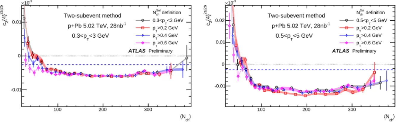
Figure 2 shows that the c

{ 4 } values from the two-subevent method are closer to each other among di ff erent event class definitions. The c

{ 4 } values decrease gradually with ⟨ N

⟩ and become negative for

ch〉

〈N

50 100 150 200

2a|2b {4}2c

0 0.01 0.02

10-3

×

ATLAS Preliminary Two-subevent method

pp 13 TeV, 0.9pb-1

<3 GeV 0.3<pT

definition

Sel

Nch

<3 GeV 0.3<pT

>0.2 GeV

T

p

>0.4 GeV pT

>0.6 GeV pT

ch〉

〈N

50 100 150 200

2a|2b{4}2c

0 0.02 0.04 0.06

10-3

×

ATLAS Preliminary Two-subevent method

pp 13 TeV, 0.9pb-1

<5 GeV 0.5<pT

definition

Sel

Nch

<5 GeV 0.5<pT

>0.2 GeV

T

p

>0.4 GeV pT

>0.6 GeV pT

Figure 2: The c

{ 4 } calculated for charged particles with 0.3 < p

< 3 GeV (left panel) or 0.5 < p

< 5 GeV (right panel) with the two-subevent cumulant method from the 13 TeV pp data. The event averaging is performed for N

calculated for various p

selections as indicated in the figure, which is then mapped to ⟨ N

⟩ , the average number of charged particles with p

> 0.4 GeV. The dashed line indicates the c

{ 4 } value corresponding to a 4% v

signal.

⟨ N

⟩ > 70 when c

{ 4 } is calculated in 0.3 < p

< 3 GeV and for ⟨ N

⟩ > 150 when c

{ 4 } is calculated in 0.5 < p

< 5 GeV. Therefore the c

{ 4 } values from the two-subevent method are more sensitive to genuine long-range ridge correlations, but nevertheless are still a ff ected by non-flow, especially in the low ⟨ N

⟩ region, and for higher p

.

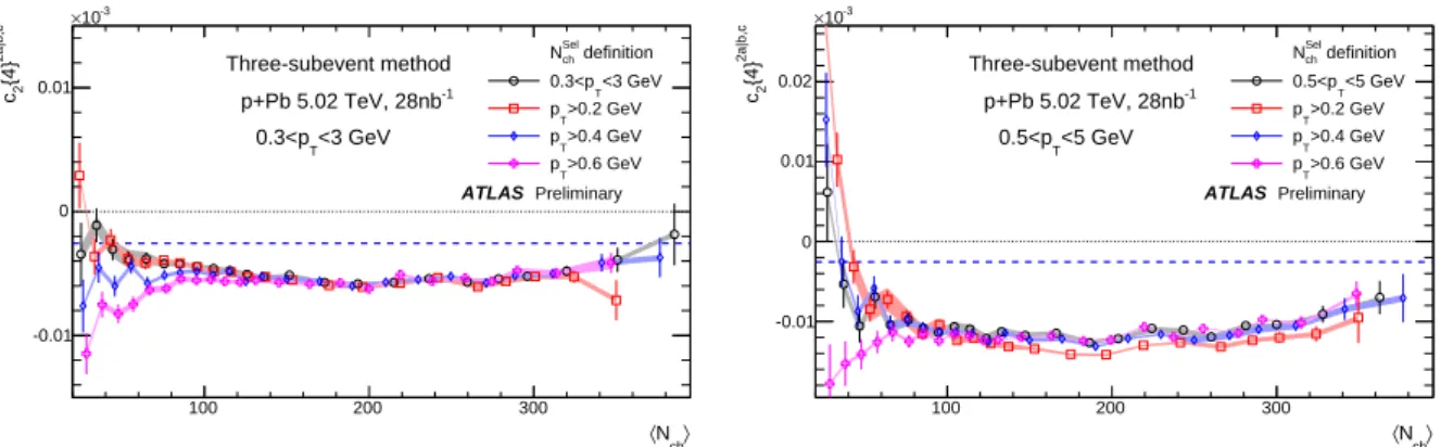
Figure 3 shows the results from the three-subevent method. For most of the ⟨ N

⟩ range, the c

{ 4 } values are negative, i.e. having the “correct” sign expected for long-range ridge. The c

{ 4 } values show some sensitivity on reference N

but they are close to each other for all definitions in the region

⟨ N

⟩ > 100. This suggests that the residual non-flow may still be important at small ⟨ N

⟩ , but is

negligible at ⟨ N

⟩ > 100. It is also observed that the c

{ 4 } values for 0.5 < p

< 5 GeV are more negative than that for 0.3 < p

< 3 GeV, which is consistent with the observation that the v

associated with the long-range collectivity increases with p

[11, 15].

ch〉

〈N

50 100 150 200

2a|b,c {4}2c

-0.01 0 0.01 0.02

10-3

×

ATLAS Preliminary Three-subevent method

pp 13 TeV, 0.9pb-1

<3 GeV 0.3<pT

definition

Sel

Nch

<3 GeV

T

0.3<p

>0.2 GeV pT

>0.4 GeV

T

p

>0.6 GeV

T

p

ch〉

〈N

50 100 150 200

2a|b,c{4}2c

0 0.02 0.04 0.06

10-3

×

ATLAS Preliminary Three-subevent method

pp 13 TeV, 0.9pb-1

<5 GeV 0.5<pT

definition

Sel

Nch

<5 GeV

T

0.5<p

>0.2 GeV pT

>0.4 GeV

T

p

>0.6 GeV

T

p

Figure 3: The c

{ 4 } calculated for charged particles with 0.3 < p

< 3 GeV (left panel) or 0.5 < p

< 5 GeV (right panel) with the three-subevent cumulant method from the 13 TeV pp data. The event averaging is performed for N

calculated for various p

selections as indicated in the figure, which is then mapped to ⟨ N

⟩ , the average number of charged particles with p

> 0.4 GeV. The dashed line indicates the c

{ 4 } value corresponding to a 4%

v

signal.

Given the relatively small sensitivity of the c

{ 4 } on the reference N

in the three-subevent method, the remaining discussion focuses on cases where the reference N

is calculated in the same p

as that used for calculating c

{ 4 } , i.e. 0.3 < p

< 3 GeV and 0.5 < p

< 5 GeV.

7.2 Comparison between di ff erent cumulant methods

ch〉

〈N

50 100 150 200

{4}2c

-5 0 5 10 15×10^-6

ATLAS Preliminary pp 13 TeV, 0.9pb-1

<3 GeV 0.3<pT

<3 GeV for 0.3<pT Sel

Nch

Standard 2-subevent 3-subevent

ch〉

〈N

50 100 150 200

{4}2c

0 0.02 0.04

10-3

×

ATLAS Preliminary pp 13 TeV, 0.9pb-1

<5 GeV 0.5<pT

<5 GeV for 0.5<pT Sel

Nch

Standard 2-subevent 3-subevent

Figure 4: The c

{ 4 } calculated for charged particles with 0.3 < p

< 3 GeV (left panel) or 0.5 < p

< 5 GeV (right panel) compared between the three cumulant methods from the 13 TeV pp data. The event averaging is performed for N

calculated for same p

range, which is then mapped to ⟨ N

⟩ , the average number of charged particles with p

> 0.4 GeV. The dashed line indicates the c

{ 4 } value corresponding to a 4% v

signal.

Figures 4–6 show direct comparisons of the results between the three methods for pp collisions at √ s = 13 TeV, pp at √

s = 5.02 TeV and p +Pb collisions at √ s

= 5.02 TeV, respectively. The results

from 5.02 TeV pp collisions are similar to those from the 13 TeV pp collisions, i.e. the c

{ 4 } values are

ch〉

〈N

50 100

{4}2c

0 0.01 0.02 0.03 0.04

10-3

×

ATLAS Preliminary pp 5.02 TeV, 0.17 pb-1

<3 GeV 0.3<pT

<3 GeV for 0.3<pT Sel

Nch

Standard 2-subevent 3-subevent

ch〉

〈N

50 100

{4}2c

0 0.05 0.1

10-3

×

ATLAS Preliminary pp 5.02 TeV, 0.17 pb-1

<5 GeV 0.5<pT

<5 GeV for 0.5<pT Sel

Nch

Standard 2-subevent 3-subevent

Figure 5: The c

{ 4 } calculated for charged particles with 0.3 < p

< 3 GeV (left panel) or 0.5 < p

< 5 GeV (right panel) compared between the three cumulant methods from the 5.02 TeV pp data. The event averaging is performed for N

calculated for same p

range, which is then mapped to ⟨ N

⟩ , the average number of charged particles with p

> 0.4 GeV. The dashed line indicates the c

{ 4 } value corresponding to a 4% v

signal.

ch〉

〈N

100 200 300

{4}2c

-0.01 0 0.01

10-3

×

ATLAS Preliminary p+Pb 5.02 TeV, 28nb-1

<3 GeV 0.3<pT

<3 GeV for 0.3<pT Sel

Nch

Standard 2-subevent 3-subevent

ch〉

〈N

100 200 300

{4}2c

-0.02 0 0.02 0.04

10-3

×

ATLAS Preliminary p+Pb 5.02 TeV, 28nb-1

<5 GeV 0.5<pT

<5 GeV for 0.5<pT Sel

Nch

Standard 2-subevent 3-subevent

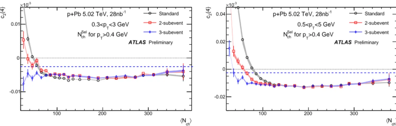
Figure 6: The c

{ 4 } calculated for charged particles with 0.3 < p

< 3 GeV (left panel) or 0.5 < p

< 5 GeV (right panel) compared between the three cumulant methods from the 5.02 TeV p+Pb data. The event averaging is performed for N

calculated for same p

range, which is then mapped to ⟨ N

⟩ , the average number of charged particles with p

> 0.4 GeV. The dashed line indicates the c

{ 4 } value corresponding to a 4% v

signal.

smallest for the three-subevent method and are largest for the standard method. The hierarchy between the three methods is also observed in p + Pb collisions, but it is limited to the low ⟨ N

⟩ region, suggesting that the influences of non-flow in p +Pb collisions are much smaller than those in pp collisions at comparable

⟨ N

⟩ . In p + Pb collisions, all three methods give consistent results for ⟨ N

⟩ > 100. Furthermore, the three-subevent method gives negative c

{ 4 } values in most of the measured ⟨ N

⟩ range.

Figures 7 and 8 compare the c

{ 4 } values between the three collision systems obtained with the standard

method and the three-subevent method. The large positive c

{ 4 } values observed in small ⟨ N

⟩ region

in the standard method are possibly due to non-flow correlations, since these are clearly absent in the

three-subevent cumulant method. In p +Pb collisions, the absolute magnitude of c

{ 4 } seems to decrease

slightly for ⟨ N

⟩ > 200 region.

ch〉

〈N 102

{4}2c

-5 0 5

10-6

×

ATLAS Preliminary

<3 GeV 0.3<pT

Standard method

ch〉

〈N 102

ATLAS Preliminary

<3 GeV 0.3<pT

Three-subevent method

=5.02 TeV s

pp

=13 TeV s pp

=5.02 TeV sNN

p+Pb

Figure 7: The c

{ 4 } calculated for charged particles with 0.3 < p

< 3 GeV using the standard cumulants (left panel) and the three-subevent method (right panel) compared between 5.02 pp, 13 TeV pp and 5.02 TeV p + Pb.

The event averaging is performed for N

calculated for same p

range, which is then mapped to ⟨ N

⟩ , the average number of charged particles with p

> 0.4 GeV.

ch〉

〈N 102

{4}2c

-0.01 0 0.01 0.02 0.03

10-3

×

ATLAS Preliminary

<5 GeV 0.5<pT

Standard method

ch〉

〈N 102

ATLAS Preliminary

<5 GeV 0.5<pT

Three-subevent method

=5.02 TeV s

pp

=13 TeV s pp

=5.02 TeV sNN

p+Pb

Figure 8: The c

{ 4 } calculated for charged particles with 0.5 < p

< 5 GeV using the standard cumulants (left panel) and the three-subevent method (right panel) compared between 5.02 pp, 13 TeV pp and 5.02 TeV p+Pb.

The event averaging is performed for N

calculated for same p

range, which is then mapped to ⟨ N

⟩ , the average

number of charged particles with p

> 0.4 GeV.

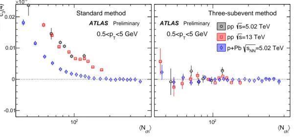
Figures 9 and 10 compare the c

{ 4 } values between the three collisions systems for the standard cumulant method and the three-subevent method. The c

{ 4 } values from the three-subevent method are consistent with zero in all three systems. For the standard method, the positive c

{ 4 } values in the small ⟨ N

⟩ region indicate the influence of non-flow correlations, but the influence is not as strong as that for c

{ 4 } .

ch〉

〈N 102

{4}3c

0 5

10-6

×

ATLAS Preliminary

<3 GeV 0.3<pT

Standard method

ch〉

〈N 102

ATLAS Preliminary

<3 GeV 0.3<pT

Three-subevent method

=5.02 TeV s

pp

=13 TeV s pp

=5.02 TeV sNN

p+Pb

Figure 9: The c

{ 4 } calculated for charged particles with 0.3 < p

< 3 GeV using the standard cumulants (left panel) and the three-subevent method (right panel) compared between 5.02 pp, 13 TeV pp and 5.02 TeV p + Pb.

The event averaging is performed for N

calculated for same p

range, which is then mapped to ⟨ N

⟩ , the average number of charged particles with p

> 0.4 GeV.

ch〉

〈N 102

{4}3c

-0.01 0 0.01 0.02

10-3

×

ATLAS Preliminary

<5 GeV 0.5<pT

Standard method

ch〉

〈N 102

ATLAS Preliminary

<5 GeV 0.5<pT

Three-subevent method

=5.02 TeV s

pp

=13 TeV s pp

=5.02 TeV sNN

p+Pb

Figure 10: The c

{ 4 } calculated for charged particles with 0.5 < p

< 5 GeV using the standard cumulants (left panel) and the three-subevent method (right panel) compared between 5.02 pp, 13 TeV pp and 5.02 TeV p + Pb.

The event averaging is performed for N

calculated for same p

range, which is then mapped to ⟨ N

⟩ , the average

number of charged particles with p

> 0.4 GeV.

7.3 Three-subevent u

{4}

From the measured c

{ 4 } , the harmonic flow v

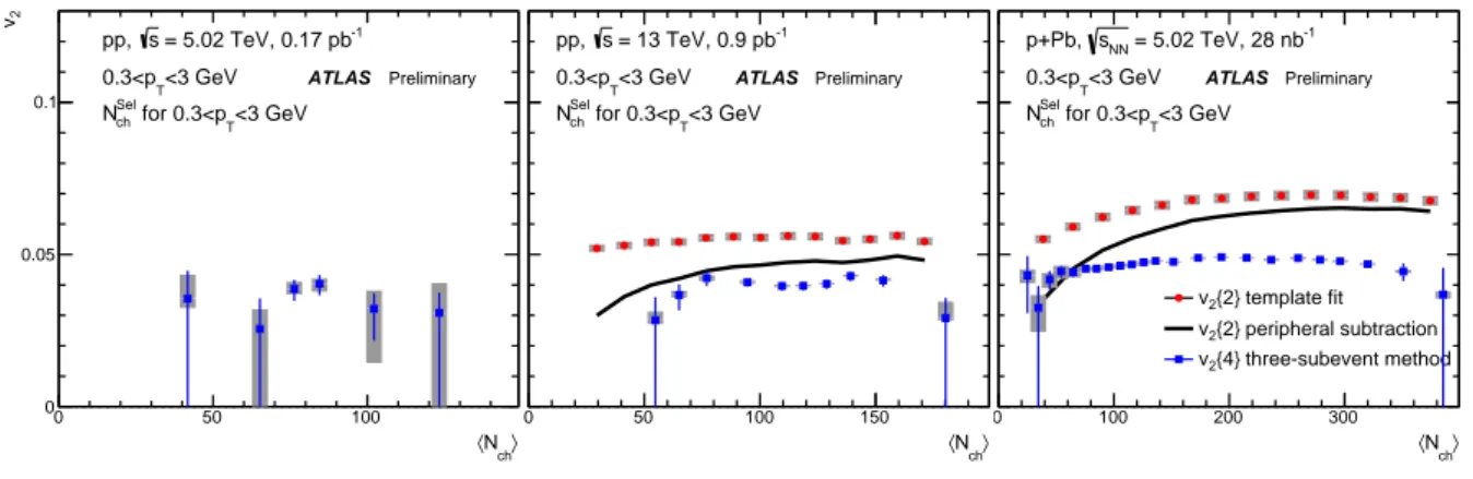
{ 4 } is obtained according to Eq. 7. Figure 11 shows the v

{ 4 } for charged particles with 0.3 < p

< 3 GeV from the three-subevent method in three collision systems. Results for the higher p

range 0.5 < p

< 5 GeV are shown in Figure 12. Significant v

{ 4 } values are observed down to ⟨ N

⟩ ≈ 50 in pp collisions and down to ⟨ N

⟩ ≈ 20–40 in p +Pb collisions.

The v

{ 4 } values are observed to be approximately independent of the ⟨ N

⟩ in the measured range in the three collision systems: 50 ≲ ⟨ N

⟩ ≲ 100 for 5.02 TeV pp, 50 ≲ ⟨ N

⟩ ≲ 150 for 13 TeV pp, and 20 ≲ ⟨ N

⟩ ≲ 300 for 5.02 TeV p +Pb, respectively. Although the much better precision of the p +Pb data suggests a slight decrease of ∣ c

{ 4 }∣ for ⟨ N

⟩ > 200 in Figs. 7 and 8.

The v

{ 4 } results are compared to the v

{ 2 } obtained from a 2PC analysis [11, 15] where the non-flow, mostly from inter-jet correlations from dijets, is estimated using low-multiplicity events ( ⟨ N

⟩ < 10) and then subtracted in the 2PC. The subtraction was done by either including or not including the pedestal in the low multiplicity events (labelled as “template fit” and “peripheral subtraction” respectively), where the pedestal is determined by a zero-yield at minimum (ZYAM) procedure [6]. Not including the pedestal in low-multiplicity events in the subtraction was shown [15] to significantly reduce the measured v

value since it explicitly assumes no long-range v

in the peripheral bin and therefore forces the v

to be zero at the lowest ⟨ N

⟩ .

ch〉

〈N

0 50 100

2v

0 0.05 0.1

= 5.02 TeV, 0.17 pb-1

s pp,

<3 GeV 0.3<pT

<3 GeV for 0.3<pT Sel

Nch

ATLAS Preliminary

ch〉

〈N

0 50 100 150

= 13 TeV, 0.9 pb-1

s pp,

<3 GeV 0.3<pT

<3 GeV for 0.3<pT Sel

Nch

ATLAS Preliminary

ch〉

〈N

0 100 200 300

= 5.02 TeV, 28 nb-1

sNN

p+Pb,

<3 GeV 0.3<pT

<3 GeV for 0.3<pT Sel

Nch

ATLAS Preliminary

template fit

2{2}

v

peripheral subtraction

2{2}

v

three-subevent method

2{4}

v

Figure 11: The v

{ 4 } calculated for charged particles with 0.3 < p

< 3 GeV using the three-subevent method in 5.02 TeV pp (left panel), 13 TeV pp (middle panel) and 5.02 TeV p + Pb collisions (right panel). They are compared to v

obtained from a two-particle correlation analysis [11,15] where the non-flow e ff ects are removed by a template fit procedure (solid circles) or with a fit after subtraction with ZYAM assumption (peripheral subtraction, solid line).

Figures 11 and 12 show that the v

{ 4 } values are smaller than the v

{ 2 } from the template-fit method in both pp and p +Pb collisions. In hydrodynamic models for small collision systems, this difference can be interpreted [39, 40] as influence of event-by-event flow fluctuations associated with fluctuating initial condition, which is closely related to the e ff ective number of sources N

for particle production in the transverse density distribution of the initial state:

v

{ 4 }

v

{ 2 } = [ 4 ( 3 + N

) ]

1/4

or N

= 4v

{ 2 }

v

{ 4 }

− 3 , (14)

Figure 13 shows the extracted N

values as a function of ⟨ N

⟩ in 13 TeV pp and 5.02 p + Pb collisions,

using the model assumption given in Eq. 14, estimated with charged particles in 0.3 < p

< 3 GeV and

ch〉

〈N

0 50 100

2v

0 0.05 0.1

= 5.02 TeV, 0.17 pb-1

s pp,

<5 GeV 0.5<pT

<5 GeV for 0.5<pT Sel

Nch

ATLAS Preliminary

ch〉

〈N

0 50 100 150

= 13 TeV, 0.9 pb-1

s pp,

<5 GeV 0.5<pT

<5 GeV for 0.5<pT Sel

Nch

ATLAS Preliminary

ch〉

〈N

0 100 200 300

= 5.02 TeV, 28 nb-1

sNN

p+Pb,

<5 GeV 0.5<pT

<5 GeV for 0.5<pT Sel

Nch

ATLAS Preliminary

template fit

2{2}

v

peripheral subtraction

2{2}

v

three-subevent method

2{4}

v

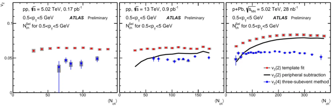
Figure 12: The v

{ 4 } calculated for charged particles with 0.5 < p

< 5 GeV using the three-subevent method in 5.02 TeV pp (left panel), 13 TeV pp (middle panel) and 5.02 TeV p + Pb collisions (right panel). They are compared to v

obtained from a two-particle correlation analysis [11,15] where the non-flow e ff ects are removed by a template fit procedure (solid circles) or with a fit after subtraction with ZYAM assumption (peripheral subtraction, solid line).

0.5 < p

< 5 GeV ranges. The extracted number of sources increases with ⟨ N

⟩ in p +Pb collisions up to N

∼ 20 in the highest multiplicity class, and it is consistent between the two p

ranges. In the model framework of Ref. [39, 40], the flow fluctuations are expected to approach a Gaussian shape for large N

, and ∣ c

{ 4 }∣ or v

{ 4 } is expected to decrease. This may be consistent with the slight decrease of ∣ c

{ 4 }∣

shown in Figs. 7 and 8 for ⟨ N

⟩ > 200. The results for 13 TeV pp collisions cover a much more limited

⟨ N

⟩ range, but are consistent with p + Pb collisions at a comparable ⟨ N

⟩ value.

ch〉

〈N

0 100 200 300

sN

0 10 20

ATLAS Preliminary

<3 GeV 0.3<pT

<3 GeV for 0.3<pT Sel

Nch

=13 TeV s pp

=5.02 TeV sNN

p+Pb

ch〉

〈N

0 100 200 300

sN

0 10 20

ATLAS Preliminary

<5 GeV 0.5<pT

<5 GeV for 0.5<pT Sel

Nch

=13 TeV s pp

=5.02 TeV sNN

p+Pb

Figure 13: The number of sources inferred from v

{ 2 } and v

{ 4 } via the model framework of Ref. [39, 40] and

Eq. 14 in 13 TeV pp and 5.02 TeV p + Pb collisions, for charged particles with 0.3 < p

< 3 GeV (left panel) and

0.5 < p

< 5 GeV (right panel).

8 Summary

Measurements of the four-particle cumulants and elliptic flow coefficients c

{ 4 } and v

{ 4 } for charged particles are presented using 0.17 pb

of pp data at √

s = 5.02 TeV, 0.9 pb

of pp data at √ s = 13 TeV and 28 nb

p +Pb of data at √ s

= 5.02 TeV. The c

{ 4 } values are calculated using the standard cumulant method and the recently proposed two-subevent and the three-subevent methods. They are all presented as a function of the average number of charged particles with p

> 0.4 GeV, ⟨ N

⟩ . It is found that the c

{ 4 } from the standard method is sensitive to the choice of particles used to form the event classes used for averaging. This sensitivity is greatly reduced in the two-subevent method and is almost fully removed in the three-subevent method, suggesting that the three-subevent method is much more ro- bust against non-flow e ff ects. A negative c

{ 4 } is obtained in all three collision systems in a broad range of ⟨ N

⟩ using the three-subevent method. The magnitude of c

{ 4 } is nearly independent of ⟨ N

⟩ but a slight decrease is observed in p + Pb collisions in the large multiplicity region. The single-particle har- monic coe ffi cient v

{ 4 } = (− c

{ 4 })

is calculated and compared with v

{ 2 } obtained previously using a two-particle correlation method, where the non-flow contributions were estimated and subtracted. The magnitude of v

{ 4 } is smaller than v

{ 2 } , as expected for a long-range collective e ff ect, and the ratio of v

{ 4 } to v

{ 2 } is used, in a model-dependent framework, to infer the number of particle-emitting sources in the initial state geometric configuration. The number of sources extracted within this framework is found to increase with ⟨ N

⟩ in p + Pb collisions. The four-particle cumulant triangular flow coe ffi cient c

{ 4 } is also extracted, and its value is found to be consistent with zero in all collision systems.

References

[1] STAR Collaboration, B. I. Abelev et al., Phys. Rev. C 80 (2009) 064912, arXiv:0909.0191 [nucl-ex].

[2] PHOBOS Collaboration, B. Alver et al., Phys. Rev. Lett. 104 (2010) 062301, arXiv:0903.2811 [nucl-ex].

[3] ALICE Collaboration, K. Aamodt et al., Phys. Rev. Lett. 107 (2011) 032301, arXiv:1105.3865 [nucl-ex].

[4] ATLAS Collaboration, Phys. Rev. C 86 (2012) 014907, arXiv:1203.3087 [hep-ex].

[5] CMS Collaboration, Phys. Rev. C 89 (2014) 044906, arXiv:1310.8651 [nucl-ex].

[6] PHENIX Collaboration, A. Adare et al., Phys. Rev. C 78 (2008) 014901, arXiv:0801.4545 [nucl-ex].

[7] CMS Collaboration, Phys. Lett. B 718 (2013) 795, arXiv:1210.5482 [nucl-ex].

[8] ALICE Collaboration, B. Abelev et al., Phys. Lett. B 719 (2013) 29, arXiv:1212.2001 [nucl-ex].

[9] ATLAS Collaboration, Phys. Rev. Lett. 110 (2013) 182302, arXiv:1212.5198 [hep-ex].

[10] PHENIX Collaboration, A. Adare et al., Phys. Rev. Lett. 111 (2013) 212301, arXiv:1303.1794 [nucl-ex].

[11] ATLAS Collaboration, Phys. Rev. C 90 (2014) 044906, arXiv:1409.1792 [hep-ex].

[12] CMS Collaboration, Phys. Rev. Lett. 115 (2015) 012301, arXiv:1502.05382 [nucl-ex].

[13] CMS Collaboration, JHEP 1009 (2010) 091, arXiv:1009.4122 [hep-ex].

[14] ATLAS Collaboration, Phys. Rev. Lett. 116 (2016) 172301, arXiv:1509.04776 [hep-ex].

[15] ATLAS Collaboration, arXiv:1609.06213 [nucl-ex].

[16] ATLAS Collaboration, ATLAS-CONF-2016-106, https://cds.cern.ch/record/2220374.

[17] P. Bozek and W. Broniowski, Phys. Rev. C 88 (2013) 014903, arXiv:1304.3044 [nucl-th].

[18] K. Dusling and R. Venugopalan, Phys. Rev. D 87 (2013) 094034, arXiv:1302.7018 [hep-ph].

[19] CMS Collaboration, Phys. Lett. B 765 (2017) 193, arXiv:1606.06198 [nucl-ex].

[20] N. Borghini, P. M. Dinh, and J.-Y. Ollitrault, Phys. Rev. C 63 (2001) 054906, arXiv:nucl-th/0007063 [nucl-th].

[21] ATLAS Collaboration, Phys. Lett. B 725 (2013) 60, arXiv:1303.2084 [hep-ex].

[22] J. Jia, M. Zhou, and A. Trzupek, arXiv:1701.03830 [nucl-th].

[23] A. Bilandzic, R. Snellings, and S. Voloshin, Phys. Rev. C 83 (2011) 044913, arXiv:1010.0233 [nucl-ex].

[24] A. Bilandzic, C. H. Christensen, K. Gulbrandsen, A. Hansen, and Y. Zhou, Phys. Rev. C 89 (2014) 064904, arXiv:1312.3572 [nucl-ex].

[25] ALICE Collaboration, B. B. Abelev et al., Phys. Rev. C 90 (2014) 054901, arXiv:1406.2474 [nucl-ex].

[26] ATLAS Collaboration, JINST 3 (2008) S08003.

[27] ATLAS Collaboration, Eur. Phys. J. C 70 (2010) 787, arXiv:1004.5293 [physics-ins-det].

[28] ATLAS Collaboration, ATLAS-LHCC-2010-013. ATLAS-TDR-19, https://cds.cern.ch/record/1291633.

[29] ATLAS Collaboration, ATLAS-LHCC-2012-009. ATLAS-TDR-19-ADD-1, https://cds.cern.ch/record/1451888.

[30] ATLAS Collaboration, Eur. Phys. J. C 72 (2012) 1849, arXiv:1110.1530 [hep-ex].

[31] ATLAS Collaboration, Phys. Lett. B 758 (2016) 67, arXiv:1602.01633 [hep-ex].

[32] ATLAS Collaboration, ATLAS-CONF-2013-104, https://cds.cern.ch/record/1624013.

[33] M. Gyulassy and X.-N. Wang, Comput. Phys. Commun. 83 (1994) 307, arXiv:nucl-th/9502021 [nucl-th].

[34] T. Sjostrand, S. Mrenna, and P. Z. Skands, Comput. Phys. Commun. 178 (2008) 852, arXiv:0710.3820 [hep-ph].

[35] ATLAS Collaboration, ATLAS-PHYS-PUB-2011-009, https://cds.cern.ch/record/1363300.

[36] GEANT4 Collaboration, S. Agostinelli et al., Nucl. Instrum. Meth. A 506 (2003) 250.

[37] ATLAS Collaboration, Eur. Phys. J. C 70 (2010) 823, arXiv:1005.4568 [physics].

[38] ATLAS Collaboration, arXiv:1606.08170 [hep-ex].

[39] A. Bzdak, P. Bozek, and L. McLerran, Nucl. Phys. A 927 (2014) 15, arXiv:1311.7325 [hep-ph].

[40] L. Yan and J.-Y. Ollitrault, Phys. Rev. Lett. 112 (2014) 082301, arXiv:1312.6555 [nucl-th].