collisions with the ATLAS detector

ATLAS-CONF-2020-042 14August2020

ATLAS CONF Note

ATLAS-CONF-2020-042

28th July 2020

Measurements of differential cross-sections in four-lepton events in 13 TeV proton–proton

collisions with the ATLAS detector

The ATLAS Collaboration

Measurements of four-lepton differential and integrated fiducial cross-sections in events with two same-flavour, opposite-charge electron or muon pairs are presented. The data correspond to 139 fb

of

√ s = 13 TeV proton–proton collisions, collected by the ATLAS detector during Run 2 of the Large Hadron Collider (2015–2018). The final-state has contributions from a number of interesting Standard Model processes that dominate in different four-lepton invariant mass regions, including single Z boson production, Higgs boson production and on-shell Z Z production, with a complex mix of interference terms, and possible contributions from beyond-the-Standard Model physics. The differential cross-sections include the four-lepton invariant mass inclusively, in slices of other kinematic variables, and in different lepton flavour categories. Also measured are di-lepton invariant masses, transverse momenta, and angular correlation variables, in four regions of four-lepton invariant mass, each dominated by different processes. The measurements are corrected for detector effects and are compared to state-of-the-art Standard Model calculations, which are found to be consistent with the data. The Z → 4 ` branching fraction is extracted, giving a value of ( 4 . 41 ± 0 . 30 ) × 10

. Constraints on a model based on a spontaneously broken B-L gauge symmetry are also evaluated.

© 2020 CERN for the benefit of the ATLAS Collaboration.

Reproduction of this article or parts of it is allowed as specified in the CC-BY-4.0 license.

1 Introduction

This note presents measurements of differential and integrated fiducial cross-sections of four-lepton events, containing two same-flavour, opposite-charge electron or muon pairs. The data used correspond to 139 fb

of

√ s = 13 TeV proton–proton collisions, collected by the ATLAS detector during Run 2 of the Large

Hadron Collider (LHC) between 2015 and 2018.

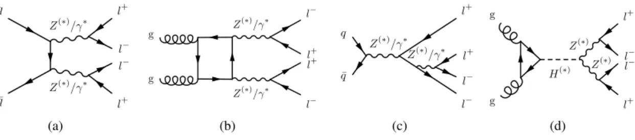
Several interesting Standard Model (SM) processes contribute to this final state, with the possibility of additional contributions from beyond the SM (BSM) physics. The dominant SM contribution is from the quark-induced t -channel q q ¯ → 4 ` process, shown in Figure 1(a). Gluon-induced gg → 4 ` production contributes at next-to-next-to-leading order (NNLO) in QCD, via a quark loop, as shown in Figure 1(b).

The Z → 4 ` process, shown in Figure 1(c), dominates in the four-lepton invariant mass, m

, region close to the Z boson mass, m

. The H → Z

Z

→ 4 ` process, shown in Figure 1(d) for the gluon–gluon production mode, dominates in the m

region close to the Higgs boson mass, m

. Here the superscript (∗) refers to a particle that can be either on-shell or off-shell.

BSM contributions can arise from modifications to the SM couplings of the Higgs boson, the gauge bosons and from possible four-fermion interactions. Contributions are also possible from models producing four leptons either via the decay of Z bosons or of new BSM particles. For example, cascade decays of new particles introduced by the Minimal Supersymmetric SM, with parameters set such that searches based on missing transverse momentum [1] are insensitive, can nevertheless contribute to four-lepton final states [2].

Other examples include generic models with additional gauge boson(s), Z

, which may be pair-produced and decay to lepton pairs, or models with additional Higgs bosons which may decay to Z Z .

Z^(∗)/γ^∗

Z^(∗)/γ^∗

¯ q q

l⁺ l⁻ l⁻ l⁺

(a)

Z^(∗)/γ^∗ Z^(∗)/γ^∗

g g

l⁻ l⁺ l⁺ l⁻

(b)

¯ q q

l⁻ l⁺

Z^(∗)/γ^∗ Z^(∗)/γ^∗

l⁻ l⁺

(c)

H^(∗) Z^(∗) Z^(∗)

g g

l⁺ l⁻ l⁻ l⁺

(d)

Figure 1: Main contributions to thepp→4`(`=e, µ)process: (a)t-channelqq¯→4`production, (b) gluon-induced gg →4`production via a quark loop, (c) internal conversion inZ boson decays and (d) Higgs boson mediated s-channel production (here: gluon–gluon fusion). The superscript(∗)refers to particle that can be either on-shell or off-shell, where-as∗indicates that it is always off-shell.

The measurements are corrected for the effects of the detector and are defined in terms of final-state particles, rather than in terms of a particular process. The definition is inclusive of particles in addition to the two lepton pairs, including neutrinos, other leptons, hadrons, photons and any possible BSM particles, although the leptons are required to be isolated from other particles. There are therefore small SM contributions from top-quark pair production in association with a di-lepton pair, from tri-boson processes, where at least two bosons decay leptonically, and from events where τ leptons decay to muons or electrons. Using this definition results in minimal dependence on the measurement from the modelling of these other SM processes. The dependence on SM modelling is transferred to the theoretical predictions that are used to compare to the data.

Cross-sections are measured differentially as a function of various kinematic variables and integrated fiducial

cross-sections are also provided. The primary observable, m

, is measured inclusively, sliced in other

kinematic variables, and in different lepton flavour categories. Additional differential cross-sections are measured, including di-lepton invariant masses and transverse momenta, and angular correlation variables between leptons, in four regions of m

, each dominated by different processes. The m

distributions and a subset of the other variables measured in the m

region above the on-shell Z Z production threshold, have been previously presented at this centre-of-mass energy, using a smaller dataset [3–5]. The current result is more inclusive than previous measurements, in particular the previous requirements that the invariant mass of at least one of the di-lepton pairs be close to m

is removed. This gives sensitivity to BSM processes where there are sources of di-lepton pairs other than Z boson decays. The cross-section measurement in the region close to the Z mass is used to extract the Z → 4 ` branching fraction.

BSM contributions to this final-state may lead to discrepancies between the measured cross-sections and the SM predictions. The measurements can therefore be used to set limits on a wide range of BSM models.

The methods used to correct the data for the effects of the detector are shown to be robust against the addition of BSM contributions, as is discussed in Section 5.4. Since the cross-sections are defined at particle-level they can be compared to BSM theory predictions or improved SM predictions without the need to simulate the ATLAS detector.

2 ATLAS detector

The ATLAS detector [6] at the LHC covers nearly the entire solid angle around the collision point.

It consists of an inner tracking detector (ID) surrounded by a thin superconducting solenoid, electromagnetic and hadronic calorimeters, and a muon spectrometer incorporating three large superconducting toroidal magnets.

The ID, immersed in a 2 T axial magnetic field, provides charged-particle tracking for |η| < 2 . 5. It consists of a high-granularity silicon pixel detector covering the vertex region and typically provides four measurements per track. This is followed by the silicon microstrip tracker (SCT), which usually provides eight measurements per track. These silicon detectors are complemented by the transition radiation tracker (TRT), which enables radially extended track reconstruction up to |η| = 2 . 0. The TRT also provides electron identification information based on the fraction of hits (typically 30 in total) above a higher energy-deposit threshold corresponding to transition radiation.

The calorimeter system covers the pseudorapidity range |η| < 4 . 9. Within |η| < 3 . 2, electromagnetic calorimetry is provided by barrel and endcap high-granularity lead/liquid-argon (LAr) calorimeters, with an additional thin LAr presampler covering |η| < 1 . 8, to correct for energy loss in material upstream of the calorimeters. Hadronic calorimetry is provided by the steel/scintillating-tile calorimeter, segmented into three barrel structures within |η| < 1 . 7, and two copper/LAr hadronic endcap calorimeters covering 1 . 5 < |η| < 3 . 2. The solid angle coverage is completed with forward copper/LAr and tungsten/LAr

calorimeter modules optimised for electromagnetic and hadronic measurements respectively.

1ATLAS uses a right-handed coordinate system with its origin at the nominal interaction point (IP) in the centre of the detector and thez-axis along the beam pipe. Thex-axis points from the IP to the centre of the LHC ring, and they-axis points upwards.

Cylindrical coordinates(r, φ)are used in the transverse plane,φbeing the azimuthal angle around thez-axis. The rapidity is defined asy=¹₂ln

_E+p

z E−pz

, whereEis the energy of a particle andp_zis the momentum component in the beam direction.

The pseudorapidity is defined in terms of the polar angleθasη=−ln tan(θ/2). Angular distance is measured in units of

∆R≡p

(∆η)2+(∆φ)2.

The muon spectrometer (MS) comprises separate trigger and high-precision tracking chambers measuring the deflection of muons in a magnetic field generated by superconducting air-core toroids. A set of precision chambers covers the region |η | < 2 . 7 with three layers of monitored drift tubes, complemented by cathode-strip chambers in the forward region, where the background is highest. The muon trigger system covers the region |η| < 2 . 4 with resistive-plate chambers in the barrel, and thin-gap chambers in the endcap regions.

Interesting events are selected by the first-level trigger system implemented in custom hardware, followed by algorithms implemented in software in the high-level trigger [7].

3 Fiducial region definition and measured variables

3.1 Fiducial definition

The fiducial phase space is defined according to the kinematic acceptance of the detector, with kinematics that ensure a high efficiency to trigger on the events, and is designed to be as inclusive as possible while keeping backgrounds from non-prompt leptons relatively small. The kinematic selection is defined at particle-level

using final-state, prompt

leptons (including those from τ lepton decays). Prompt electrons are “dressed” by adding to their four-momenta the four-momenta of prompt photons within a cone size of

∆R = 0 . 1. This is done because the experimental measurement of electron energies in the calorimeter includes the energy of close-by photons. If the photon is near more than one electron it is assigned to the nearest. This dressing is not applied to prompt muons as their four-momenta are measured using the ID and the MS, and the four-momenta of close-by photons are not included in the measurement. Prompt-leptons are required to be isolated from other particles by forming a scalar sum of the transverse momentum, p

, of all charged particles within a cone of ∆R = 0 . 3 of the lepton. The ratio of this sum to the p

of the lepton is required to be less than 0.16. If another selected lepton is within the cone, the momentum of this lepton is not included in the sum.

Electrons (muons) are required to have p

> 7 ( 5 ) GeV and |η| < 2 . 47 ( 2 . 7 ) . Events are required to contain at least four such leptons that can be formed into at least two same-flavour, opposite-charge pairs. This results in three possible flavour configurations: e

e

e

e

(4 e ), e

e

µ

µ

(2 e 2 µ ) and µ

µ

µ

µ

(4 µ ).

Additional particles (leptons, neutrinos, photons, hadrons and possible BSM particles) are allowed to be present in the event. Events are also required to satisfy the following:

• p

> 20 GeV for the leading lepton (in p

).

• p

> 10 GeV for the sub-leading lepton (in p

).

• The invariant mass of any same-flavour, opposite-charge lepton pair that can be formed in the event is required to exceed m

> 5 GeV.

• The angular separation between any two leptons in the event is required to exceed ∆R > 0 . 05.

These requirements are made to minimise experimental uncertainties and are justified in Section 5.1.

2Particle-level refers to a definition based on final-state particles equivalent to the particles produced from a Monte Carlo event generator simulation, without simulating the effects of the detector. The data are corrected to this level such that they can be compared directly to theoretical predictions.

3Prompt refers to leptons and photons that do not originate from hadron decays. This excludes leptons originating from hadronic resonances such asJ/ψ→`<sup>+</sup>`⁻andΥ→`<sup>+</sup>`⁻[8].

3.2 Lepton pairing

Leptons are paired in order to define some of the measured variables. The same-flavour, opposite-charge pair with an invariant mass closest to m

is selected as the primary pair in the event. Of the remaining leptons, the same-flavour, opposite-charge pair with an invariant mass closest to m

is selected as the secondary pair, completing a quadruplet of leptons. Therefore, only one quadruplet is defined even in events containing more than four leptons. This selection strategy ensures that pairs corresponding to on-shell Z bosons for the dominant Z Z pair production process are preferentially formed.

3.3 Measured variables

The integrated fiducial cross-section is measured over the full fiducial phase-space and in four m

regions dominated by: single Z boson production (60 < m

< 100 GeV), Higgs boson production (120 < m

< 130 GeV), on-shell Z Z production (180 < m

< 2000 GeV) and off-shell Z Z production (20 < m

< 60 GeV or 100 < m

< 120 GeV or 130 < m

< 180 GeV).

A number of differential fiducial cross-sections are also measured, providing kinematic information about the events sensitive to the modelling of the SM processes, including QCD and electroweak corrections, and to possible BSM contributions. The main observable of this measurement is the invariant mass of the four leptons in the quadruplet, m

. The distribution is measured single-differentially as well as differentially in slices of the four-lepton transverse momentum, p

T

, and the absolute four-lepton rapidity, | y

|. The single-differential m

distribution is also measured in 4 e , 4 µ and 2 e 2 µ events separately.

The following variables are measured in the four regions of m

defined above:

• The invariant mass of the primary (secondary) lepton pair: m

( m

).

• The transverse momentum of the primary (secondary) lepton pair: p

( p

).

• A variable sensitive to the polarisation of the decaying particle: cos θ

12(34)

is the cosine of the angle between the negative lepton in the primary (secondary) di-lepton rest frame, and the primary (secondary) di-lepton pair in the laboratory frame.

• The absolute rapidity difference between the primary and secondary lepton pairs, |∆y

| .

• The difference in the azimuthal angle between the primary and secondary lepton pairs, |∆φ

| .

• The difference in the azimuthal angle between the leading lepton and sub-leading lepton of the quadruplet, |∆φ

| .

4 Theoretical predictions and simulation

Simulated events are used to correct the observed events for detector effects, as well as to provide the particle-level predictions with systematic uncertainties to compare with the measured data. The various simulated samples and their uncertainties are described in this section.

The q q ¯ → 4 ` process, including Z → 4 ` , is simulated with the Sherpa v2.2.2 event generator [9]. Matrix

elements are calculated at next-to-leading order (NLO) accuracy in QCD for up to one additional parton and

at leading order (LO) accuracy for up to three additional parton emissions. The higher order corrections

include initial-states with a gluon, but the q q ¯ → 4 ` notation is kept for simplicity. The calculations are matched and merged with the Sherpa parton shower based on Catani-Seymour dipole factorisation [10, 11], using the meps@nlo prescription [12–15]. The virtual QCD corrections are provided by the OpenLoops library [16, 17]. The NNPDF3.0nnlo set of PDFs is used [18], along with the dedicated set of tuned parton-shower parameters developed by the Sherpa authors. All Sherpa v2.2.2 samples discussed below use this same PDF set and tune.

An alternative q q ¯ → 4 ` sample is generated at NLO accuracy in QCD using Powheg-Box v2 [19–21].

Events are interfaced to Pythia8.186 [22] for the modelling of the parton shower, hadronisation, and underlying event, with parameters set according to the aznlo tune [23]. The CT10 PDF set [24] is used for the hard-scattering processes, whereas the CTEQ6L1 PDF set [25] is used for the parton shower. A correction to higher-order precision, defined for this process as the ratio of the cross-section at NNLO QCD accuracy to the one at NLO QCD accuracy, is obtained using a matrix NNLO QCD prediction [26–29], and applied as a function of m

.

A reweighting for virtual NLO electroweak (EW) effects [30, 31] is applied as a function of m

to both q q ¯ → 4 ` samples. A 100% uncertainty on this reweighting function is assigned to account for non- factorising effects in events with high QCD activity [32]. The real higher-order electroweak contribution to 4 ` production in association with two jets (which includes vector-boson scattering, but excludes processes involving the Higgs boson) is not included in the sample discussed above but is simulated separately with the Sherpa v2.2.2 generator. The LO-accurate matrix elements are matched to a parton shower based on Catani-Seymour dipole factorisation using the meps@lo prescription [12–15].

Uncertainties on both q q ¯ → 4 ` samples due to missing higher-order QCD corrections are evaluated [33]

using seven variations of the QCD factorisation and renormalisation scales in the matrix elements by factors of one half and two, avoiding variations in opposite directions. The envelope of these variations is taken as the uncertainty. For the Sherpa sample, uncertainties on the nominal PDF set are evaluated using 100 replica variations, as well as by reweighting to the alternative CT14nnlo [34] and MMHT2014nnlo [35]

PDF sets, and taking the envelope of these contributions as a combined PDF uncertainty. The uncertainty on the strong coupling constant α

is assessed by variations of ± 0 . 001. For the Powheg +Pythia8 sample, the PDF uncertainty is evaluated using the 26 pairs of upwards and downwards internal PDF variations within CT10 NLO , as well as reweighting to the NNPDF3.0nnlo and MSTW2008 [36] PDF sets, and taking the envelope of the variations.

The gluon-initiated 4 ` production process is simulated using Sherpa v2.2.2 [37] at LO precision for up to one additional parton emission, with the same setup used for the parton shower as the q q ¯ → 4 ` sample described above. There is a m

> 10 GeV generator cut on any same-flavour and opposite-charge lepton pair, removing a small amount of the phase-space included in the measurement. This is recovered by the reweighting procedure described below, for all but the m

and m

distributions in the region below 10 GeV, where the prediction from this sample is missing. This is a few percent of the total prediction in the fiducial phase-space in this region. The sample includes the gg → 4 ` box diagram, the s -channel process proceeding via a Higgs boson, gg → H

→ Z

Z

→ 4 ` , and the interference between the

two. In the region m

< 130 GeV, where on-shell Higgs boson production dominates, this sample is

only used to simulate the gg → 4 ` box diagram, with the dedicated samples described below used to

simulate Higgs boson production. In this region the interference between the two is negligible and is

not simulated. In the region m

> 130 GeV this sample is used to simulate all three contributions. A

NLO QCD calculation [38, 39] allowing m

differential K -factors to be calculated is used to correct each

of these contributions separately, together with an associated uncertainty. The details are the same as

those described in Ref. [3]. An additional correction factor of 1.2, taken from the ratio of a NNLO QCD

precision calculation [40, 41] to the NLO prediction for off-shell Higgs production, is assumed to be the same for all three components. Scale and PDF uncertainties are obtained in the same way as for the Sherpa q q ¯ → 4 ` sample described above.

In the region m

< 130 GeV, where on-shell Higgs boson production is important, and the effect of interference is negligible, dedicated samples are used to model the Higgs boson production processes as accurately as possible. Higgs boson production via gluon–gluon fusion [42], which dominates, is simulated at NNLO accuracy in QCD using the Powheg NNLOPS program [19, 43–46]. The simulation achieves NNLO accuracy for arbitrary inclusive gg → H observables by reweighting the Higgs boson rapidity spectrum in Hj-MiNLO [42, 47, 48] to that of HNNLO [49]. Pythia8 [50] is used. The PDF4LHC15nnlo PDF set [51] and the aznlo tune [23] of Pythia8 [50] is used. The prediction from the Monte Carlo samples is normalised to the next-to-next-to-next-to-leading order (N

LO) cross-section in QCD plus electroweak corrections at next-to-leading order (NLO) [41, 52–61]. Higgs boson production via vector-boson fusion (VBF) [62], in association with a vector boson ( V H ) [63], and in association with a top-quark pair are all simulated with Powheg [19, 45, 46, 62] and interfaced with Pythia8 [50] for parton shower and non-perturbative effects. The PDF4LHC15 PDF set [51] and the aznlo tune [23] of Pythia8 [50] are used. For VBF production, the Powheg prediction is accurate to NLO in QCD, and is normalised to an approximate-NNLO QCD cross-section with NLO electroweak corrections [64–66]. For V H production, the Powheg prediction is accurate to NLO in QCD for up to one additional jet, and is normalised to a cross-section calculated at NNLO in QCD with NLO electroweak corrections [67–71]. The uncertainties on the on-shell Higgs boson production are the same as reported in Ref. [72]. The largest components are the QCD scale and PDF uncertainties affecting the gluon–gluon fusion component.

Other smaller SM processes contributing to the final-state of the analysis include tri-boson production ( WW Z , W Z Z and Z Z Z ) collectively referred to as VVV , and t t ¯ pairs produced in association with vector bosons ( t t Z ¯ , t tWW ¯ ) collectively referred to as t tV ¯ ( V ). The production of tri-boson events is simulated with Sherpa v2.2.2 using factorised gauge boson decays. Matrix elements, accurate at NLO for the inclusive process and at LO for up to two additional parton emissions, are matched and merged with the Sherpa parton shower based on Catani-Seymour dipole factorisation using the meps@nlo prescription. The virtual QCD correction for matrix elements at NLO accuracy are provided by the OpenLoops library. The t¯ tV ( V ) samples are produced with Sherpa v2.2.0 at LO accuracy, using the meps@lo setup with up to one additional parton. The default Sherpa v2.2.0 parton shower is used along with the NNPDF3.0nnlo PDF set.

For practical reasons, uncertainties on these predictions are evaluated based on experimental uncertainties on the cross-section measurements of t t Z ¯ [73] and WW Z [74]. The former leads to a flat ± 15% uncertainty on all t tV ¯ ( V ) processes and the latter to a flat ± 40% uncertainty on all tri-boson processes.

A small contribution from double-parton scattering, with the di-lepton pairs produced in different parton- parton interactions is expected to contribute at the level of 0.1%. This is included in the definition of the final-state but is neglected from the predictions.

For the purpose of correcting for detector effects, generated events are passed through a simulation of

the ATLAS detector and trigger [75], and the same reconstruction and analysis software as applied to

the data. Corrections are applied to the simulation of leptons, to account for differences seen with the

data. These include differences in lepton reconstruction, identification, isolation and vertex-association

efficiencies, as well as momentum scale and resolution, with associated uncertainties [76, 77]. The effect

of multiple proton–proton interactions in the same bunch crossing, known as pile-up, is emulated by

overlaying inelastic proton–proton collisions, simulated with Pythia8.186 [22] using the NNPDF2.3lo set

of PDFs [78] and the A3 tune [79]. The events are then reweighted to reproduce the distribution of the

number of collisions per bunch-crossing observed in the data, with an associated uncertainty coming from the uncertainty on the inelastic cross-section.

5 Data analysis

5.1 Event Selection

Events are selected by requiring at least one of a set of triggers to be activated. Each trigger requires the presence of one, two or three electrons or muons with a variety of p

thresholds [80, 81]. The trigger efficiency increases from around 80% for m

below 80 GeV, to nearly 100% at m

∼ 200 GeV and above.

Events are required to contain at least one reconstructed pp collision vertex candidate with at least two associated ID tracks. The vertex with the largest sum of p

T

of tracks is considered to be the primary interaction vertex.

Electron identification utilises a likelihood-based method, combining information from the shower shapes of clusters in the electromagnetic calorimeters, properties of tracks in the ID, and the quality of the track–cluster matching, the latter being based on spatial separation as well the ratio of the cluster energy to the track momentum. The shower shape variables include variables sensitive to the lateral and longitudinal development of the electromagnetic shower, and variables designed to reject clusters from multiple incident particles. A loose identification working point is used [76], with the additional requirement of a hit on the innermost layer of the pixel detector. Muons are identified using information from various combinations of the MS, the ID and the calorimeters. As with electrons, a loose identification working point is used [77], which focuses on recovering efficiency in poorly instrumented detector regions. In particular, ID tracks identified as muons based on their calorimetric deposits or the presence of individual muon segments are included in the region |η| < 0 . 1, where the muon spectrometer is only partially instrumented. In addition, standalone MS tracks, supplemented using tracklets in the forward pixel detector where possible, are added in the region 2 . 5 < |η| < 2 . 7, where ID coverage does not permit full independent ID track reconstruction.

The kinematic cuts described in Section 3 for the particle-level selection are also applied to these reconstruction-level

electrons and muons, ensuring very little extrapolation into unmeasured regions when correcting for detector effects. The p

cuts on the leading and sub-leading leptons are 20 GeV and 10 GeV respectively, to ensure efficient triggering of events. The requirements of m

> 5 GeV and ∆R > 0 . 05 between the leptons suppress contributions from J/ψ decays and conversion electrons respectively. To select leptons originating from the primary proton–proton interaction, their tracks are required to have a longitudinal impact parameter, z

, satisfying | z

sin (θ)| < 0 . 5 mm from the primary interaction vertex.

For MS-only muons no such requirement is made. To avoid the double-counting of particles, if leptons share an ID track, only one survives the selection. Preference is given to higher p

leptons and muons over electrons, unless the muon has no associated MS track, in which case the electron survives. The leptons satisfying the above criteria are referred to as baseline leptons, and are used to estimate the background contribution from non-prompt leptons, as discussed in Section 5.2.

Once the quadruplet is formed, as detailed in Section 3, the following further selection requirements are made. The electrons and muons are required to be isolated from other particles using information from the

4Reconstruction-level refers to the identification and kinematic measurements of final-state object candidates, as defined by measurements with the detector, or full detector simulation, and a subsequent reconstruction software step.

ID and the calorimeters. The isolation variables have a correction for pile-up, and another correction for tracks or deposits originating from other leptons in the quadruplet, in order to retain events with close-by prompt leptons. Additionally, the transverse impact parameter significance, | d

|/σ

, calculated relative to the measured beam-line position must be less than 5 (3) for electrons (muons). The leptons satisfying the above criteria are referred to as signal leptons, and they are a subset of the baseline leptons.

The overall efficiency to reconstruct, identify, isolate and vertex-associate electrons varies from 30% at low- p

and high |η| to 98% at high- p

. For muons it varies from 30% at low- p

and high |η| to more than 99% at high- p

, and is higher on average than for electrons.

5.2 Background Estimation

Backgrounds where one or more of the reconstructed leptons entering a quadruplet did not originate from a prompt lepton are estimated using data-driven methods rather than simulation. The backgrounds are subtracted from the data prior to correcting for detector effects. Simulations suggest that the main source of background events are those where the quadruplet is formed by a combination of prompt leptons from Z /γ

or t¯ t production processes, with additional leptons originating from the decay of hadrons.

The background is estimated with a fake factor method. The method uses three classes of leptons, the signal and baseline leptons defined in Section 5.1, as well as baseline-not-signal leptons, defined as those which pass the baseline selection but fail the signal selection. A quantity called the fake factor is defined as the ratio between the number of signal leptons and the number of baseline-not-signal leptons and measured in a dedicated control region in data, which is enriched with non-prompt leptons. The background yield is estimated by applying the fake factor to each baseline-not-signal lepton in events passing an event selection requiring only baseline instead of signal leptons. Four-lepton events containing prompt baseline-not-signal leptons are removed from the estimation using simulated predictions.

The control region in which the fake factor is evaluated is defined by selecting events containing a same-flavour and opposite-charge lepton pair, with an invariant mass within 15 GeV of m

, and at least one other baseline lepton. This sample is composed of 90% Z → `` events. The remaining leptons that do not form the candidate Z pair are likely to be non-prompt and to have originated from hadron decays or, to a lesser extent, from jets mis-identified as leptons. There is a small contribution of prompt leptons, primarily from W Z decays, and an even smaller contribution from four-prompt-lepton events. These contributions are subtracted using Sherpa 2.2.2 simulations. After this subtraction, the fake factor is measured in bins of lepton p

and the number of jets in the event.

An important assumption of the fake factor method is that the probability of any given lepton to be prompt is uncorrelated with the equivalent probabilities for other leptons in the event. Since this analysis accepts leptons which are separated by as little as ∆R = 0 . 05, this assumption can break down. For example, cascade decays of b -hadrons can lead to two or more leptons being nearby. In such cases, the leptons’

prompt/non-prompt probabilities are highly correlated. To account for this, if two leptons are found to be

within ∆R < 0 . 4 of each other, one of them is omitted when determining the fake contribution expected

from that event. The choice of which lepton to omit depends on the lepton flavour and p

. If the leptons

are opposite flavour, the electron is skipped, and if the leptons are of the same flavour, the one with the

lowest transverse momentum is skipped. This approach was verified in closure tests of the method using

simulated events.

In order to limit the impact of statistical fluctuations in the background, a smoothing procedure based on a variable-span smoothing technique [82] is used to obtain a smoother background shape and reduce the impact of single outlier events. The overall predicted background is 4% of the selected data in the signal region, and varies from 38% for m

between 20 and 60 GeV, quickly falling with m

to around 2.5% for m

above 200 GeV.

The background estimation was validated in dedicated phase-space regions: The first validation region is the “different-flavour validation region”, which is defined like the signal region, but requiring one of the pairs of leptons to have different flavours. The second is the “same-charge validation region”, which instead requires one of the pairs of leptons to have the same charge. After application of the estimated background yield, the data and simulation in both validation regions are in agreement within the statistical uncertainties of the data.

Five sources of uncertainty on the background yield are considered. First, the dominant uncertainty for m

< 150 GeV and m

> 350 GeV comes from the statistical uncertainty on the data in events with four baseline-not-signal leptons, used as input to the fake factor method. Second, dominant in the region 150 < m

< 350 GeV, is the theory uncertainties on the prompt lepton subtraction in the control region, predominantly from W Z events, which are dominated by QCD scale variations. Third, the uncertainties on the subtracted contribution of genuine prompt four-lepton events containing baseline-not-signal leptons (which is estimated from simulation) are propagated to the background estimate, leading to a sizeable contribution at m

∼ 1000 GeV. Fourth is the statistical uncertainty on the data in the control region used to measure the fake factors, which is a sub-dominant contribution. Finally, a very small uncertainty on the smoothing technique is included. The total size of the uncertainty on the predicted number of background events varies between 15% for m

between 20 and 60 GeV and 150% for m

of 1000 GeV.

The above method does not account for a very small background contribution from Z + Υ events. These events amount to 0.2% of the selected data, and 0.8% in the Z → 4 ` region, and are removed using an estimate from Pythia8 simulation.

5.3 Selected Events

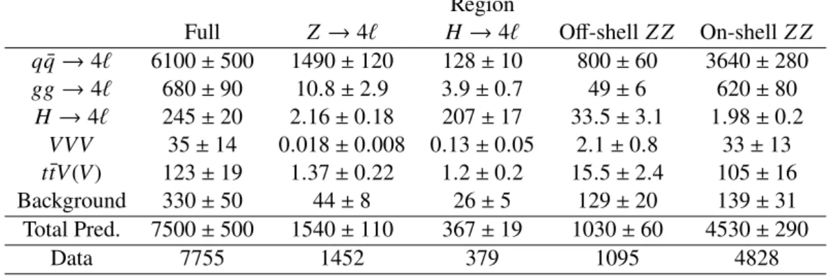
Table 1 shows the number of selected events over the full fiducial phase-space and in each m

region.

Also shown is the predicted contribution from each SM process contributing to the final state, as well the predicted background contribution from non-prompt leptons. The Sherpa simulation is used for the q q ¯ → 4 ` process. Uncertainties on the predictions arise from the sources discussed in Sections 4, 5.2 and 5.5.

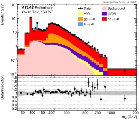
Figure 2 shows the m

distribution comparing data to these predictions at reconstruction level, together with the uncertainties. The distribution shows a number of interesting features. There is a peak in the region m

∼ m

, dominated by the Z → 4 ` process, and a peak in the region m

∼ m

, dominated by the H → 4 ` processes. At the threshold for producing two on-shell Z bosons, m

∼ 180 GeV, there is an increase in the cross-section. The cross-section then falls steeply.

5.4 Detector Corrections

After subtracting the backgrounds from non-prompt leptons, the measured cross-sections are corrected for

detector effects using a combination of a per-lepton efficiency correction and an iterative Bayesian unfolding

Table 1: Predicted reconstruction-level yields per process and in total, compared to observed data counts, over the full fiducial phase-space and in the following regions ofm₄`: Z → 4` (60 < m₄` < 100 GeV),H → 4` (120<m_{4`</sub> <130 GeV), off-shellZ Z(20<m<sub>4`} <60 GeV or 100<m_{4`</sub> <120 GeV or 130<m<sub>4`} <180 GeV) and on-shellZ Z(180<m<sub>4`</sub> <2000 GeV). Uncertainties on the predictions include both statistical and systematic sources. The uncertainty on the total prediction takes into account correlations between processes. H→4`row includes only the on-shell Higgs boson contribution, with off-shell contributions included ingg→4`.

Region

Full Z → 4 ` H → 4 ` Off-shell Z Z On-shell Z Z q q ¯ → 4 ` 6100 ± 500 1490 ± 120 128 ± 10 800 ± 60 3640 ± 280 gg → 4 ` 680 ± 90 10 . 8 ± 2 . 9 3 . 9 ± 0 . 7 49 ± 6 620 ± 80

H → 4 ` 245 ± 20 2 . 16 ± 0 . 18 207 ± 17 33 . 5 ± 3 . 1 1 . 98 ± 0 . 2 VVV 35 ± 14 0 . 018 ± 0 . 008 0 . 13 ± 0 . 05 2 . 1 ± 0 . 8 33 ± 13 t¯ tV ( V ) 123 ± 19 1 . 37 ± 0 . 22 1 . 2 ± 0 . 2 15 . 5 ± 2 . 4 105 ± 16

Background 330 ± 50 44 ± 8 26 ± 5 129 ± 20 139 ± 31

Total Pred. 7500 ± 500 1540 ± 110 367 ± 19 1030 ± 60 4530 ± 290

Data 7755 1452 379 1095 4828

technique [83]. The detector effects include the resolution of the measured kinematic variables and the inefficiencies of reconstructing leptons and of triggering on the events. The sum of the SM simulations described in Section 4 are used to provide the relationship between the particle-level observables defined in Section 3 and the reconstruction-level observables defined in Section 5.1.

The first step is a correction for the efficiency of reconstructing, identifying, isolating and vertex-associating each lepton in the quadruplet, which is referred to as a pre-unfolding efficiency correction. The efficiency is measured in the simulation as a function of η and p

for electrons and muons separately. It is defined as the ratio of the number of reconstruction-level leptons (that are matched with ∆R < 0 . 05 to particle-level leptons) to the number of particle-level leptons. A per-event weight is given by:

Î

i(pTi1,ηi)

, where

(p

, η

) is the efficiency for the i

lepton in the quadruplet, treated as uncorrelated between leptons.

This weight is applied to events in both data and simulation, taking the η and p

values from the leptons in data and simulation respectively. This ensures there is minimal dependence on the SM description of the lepton kinematics when correcting the data. This pre-unfolding correction takes into account the different efficiency for leptons from tau decays, due to a lower | d

|/σ

efficiency, based on their admixture expected from the simulation, as a function of m

.

The data are then corrected for events that pass the reconstruction-level selection but fail the particle-level

selection. This primarily occurs due to resolution effects, and is corrected by a multiplicative factor, known

as a fiducial correction, in each bin of each distribution. Then, the iterative Bayesian procedure is applied

using the SM particle-level distribution as the initial prior. The data are unfolded using a migration matrix

containing probabilities that an event in a given particle-level bin of a distribution will be found in a

particular reconstruction-level bin of that distribution. This matrix is formed from events that pass both the

particle-level and reconstruction-level event selections. This process is iterated with the prior being replaced

by the unfolded data on each iteration: three iterations are used for all distributions, with the exception of

m

, |∆ y

| and |∆φ

| where only two iterations are applied. The final step is to divide the resulting

unfolded distribution by the ratio of the number of events passing both particle- and reconstruction-level

selection to the number passing the particle-level selections. Since the reconstruction-level selections have

already had the pre-unfolding weights applied, this correction is fairly close to one, but it accounts for any

50 100 150 200 [GeV]

m4l

−2

10

−1

10 1 10 102

103

Events / GeV

103

[GeV]

m4l > 216 GeV m4l x axis logarithmic for

Data Background

VVV ttV(V)

→ 4l

gg qq → 4l

→ 4l H Preliminary

ATLAS

=13 TeV, 139 fb-1

s

50 100 150 200

0.2 0.4 0.6 0.8 1 1.2 1.4 1.6 1.8

Data/Prediction

[GeV]

m4l

300 500 700 1000 2000

Figure 2: Observed data compared to the SM prediction, using Sherpa for theqq¯→ 4`simulation, for them<sub>4`</sub>

distribution. The statistical uncertainty on the data is displayed as error bars and systematic uncertainties on the prediction are shown as a grey hashed band. The ratio of the data to the prediction is shown in the lower panel. The x-axis is on a linear scale untilm_{4`</sub> =216 GeV, when it switches to a logarithmic scale, as indicated by the double dashes on the axis. There is one additional data event reconstructed withm<sub>4`} =2.14 TeV, while 0.4 are expected from simulation form_4` >2 TeV.

residual effects such as resolution and trigger efficiencies. This is known as an efficiency correction.

For sliced variables the distributions are unfolded simultaneously, properly taking into account the migration between regions. The integrated cross-section is obtained by correcting the total number of observed events after background subtraction and pre-unfolding weights, with the fiducial and efficiency corrections calculated for the inclusive phase-space. When unfolding the per region cross-sections the inter-region migrations are accounted for.

The binning of each distribution is driven by the requirement that the fraction of events in a reconstruction- level bin that originate from the same bin at particle-level is at least 60% (70%, 80%) if there are 25 (20,14) or more events in the predicted reconstruction-level yield of the bin. These requirements ensure that the statistical uncertainties can be treated as approximately Gaussian. There is an additional constraint that bins should be centred on the various resonant peaks in the distributions.

The unfolding method is designed to minimise the dependence on the simulation of the underlying

kinematics of the particles. To validate this, a data-driven closure test is performed, where a simulated

pseudo-data sample is formed by reweighting the simulation such that the distribution agrees with the

data. This pseudo-data is then unfolded with the nominal simulation and the resulting unfolded result is

compared to the input reweighted particle-level prediction. The agreement is good and the small differences,

averaging much less than 1% but reaching 3% in a few bins in some distributions, are taken as a systematic

uncertainty on the final result.

In order to demonstrate that these measurements are robust against the presence of BSM physics in the data and can be used to constrain BSM models, a number of BSM signal injection tests are performed.

Pseudo-data consisting of SM+BSM simulations are unfolded with the nominal SM simulation and the result is compared to the particle-level SM+BSM simulation. Any differences are interpreted as a bias on the unfolded SM+BSM result. Overall the results are found to be extremely robust with only small deviations seen, all of them within the experimental uncertainties. Models that predict a broad excess over the SM prediction, such as large width resonances and modifications to SM couplings, lead to very small biases in the unfolded distributions. As an example, the addition of a heavy Higgs boson, with various Higgs masses ranging from 300 GeV to 1400 GeV, and a width of 15% of the mass, is studied. The cross-section of the process is scaled such that the change with respect to the SM prediction is equivalent to 2 σ of the data uncertainty. The bias on the unfolded result is always less than 20% of the total experimental uncertainty in any given bin, with most cases and bins being considerably less affected. Without the pre-unfolding corrections applied the bias is up to a factor of two larger, indicating that the pre-unfolding step improves the robustness of the unfolding. The same tests are performed with narrow width heavy Higgs bosons, which lead to predicted enhancements in a single bin only. These tests lead to slightly larger biases due to the more drastic changes in the predicted shapes of distributions. In this case the bias observed is still always within experimental uncertainties, with the maximum being 50% of the total experimental uncertainty in any given bin. This bias slightly reduces the cross-section in the bin of interest.

This implies that limits placed on narrow width resonances will be slightly more stringent, or claims of an excess would be slightly less significant, then they would be without the bias.

5.5 Uncertainties

The statistical uncertainty on the data is dominant for the vast majority of the differential cross-section bins.

It is estimated using 250 pseudo-datasets generated by assigning random Poisson-distributed weights of mean one to the data events, and taking the root mean square of the differences between all the unfolded results obtained using the pseduo-datasets. The statistical uncertainties obtained this way are equivalent to frequentist confidence intervals in the high-statistics limit, while in the bins with very low statistics, close to the 14 event threshold or where the data fluctuated below the threshold, the quoted bands are known to under-cover by up to 10% compared to a frequentist confidence interval.

The systematic uncertainties on the measured cross-sections are evaluated by repeating the measurement after applying each associated variation and comparing the unfolded result to the nominal. Dominant contributions arise from uncertainties on the lepton reconstruction, identification, isolation and track-to- vertex association efficiencies, and momentum resolution and scale. These uncertainties are derived from the data-driven measurements used to determine the factors applied to the simulation [76, 77], as discussed in Section 4. Another important source of uncertainty arises from the choice of generator in the simulation of the q q ¯ → 4 ` process (the nominal Sherpa prediction and the alternate Powheg + Pythia8 prediction, both introduced in Section 4) used to unfold the results. This predominantly comes from a known difference in modelling the final-state radiation of photons for the two generators. When this difference is evaluated the Powheg + Pythia8 prediction is first reweighted to match the Sherpa prediction for the distribution being unfolded. This is to avoid double counting with the data-driven closure test, described in Section 5.4.

Generally comparable in size, but larger in the tails of distributions, is the uncertainty on the estimate of the background from non-prompt leptons, as described in Section 5.2. A flat uncertainty of ± 1.7%

is assigned as a result of the uncertainty in determining the luminosity for the Run 2 dataset [84, 85].

Smaller uncertainties come from the slight non-closure in the data-driven test for the unfolding, described

in Section 5.4, the statistical uncertainty of the simulated samples, the uncertainty on the uncertainty on the inelastic cross-section, and the other theory uncertainties, the latter two both introduced in Section 4.

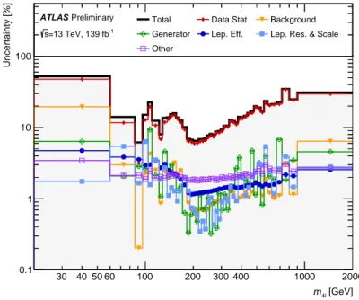
The theory uncertainties have small effects on the unfolding due to changes in the shape and normalisation of the various SM contributions. They have a much larger effect on the particle-level predictions that are compared to the data. The dominant uncertainty comes from the scale variations of each process. Figure 3 shows the breakdown of the uncertainties for the measured m

distribution. The statistical uncertainty on the data is the dominant source of uncertainty in all but the third mass bin (at m

≈ m

).

30 40 50 60 100 200 300 400 1000 2000

[GeV]

m4l

0.1 1 10 Uncertainty [%] 100

Total Data Stat. Background

Generator Lep. Eff. Lep. Res. & Scale Other

Preliminary ATLAS

=13 TeV, 139 fb-1

s

Figure 3: Uncertainty breakdown of the measured cross-section as a function ofm_4`. “Lep. Eff.” refers to the uncertainties on the lepton efficiencies, “Lep. Res. & Scale” refers to the uncertainties on the lepton resolutions and scales, the theory uncertainties are included in the “Generator” uncertainty. Contributions from the Monte Carlo statistical uncertainty and uncertainties on the luminosity and the inelastic cross-section are included in “Other”.

The dominant parts of the lepton uncertainties are highly correlated across bins. The background uncertainties are mostly uncorrelated as they are driven by limited statistics. The systematic uncertainty arising from the choice of generator is highly correlated across bins.

For the theoretical uncertainties on the particle-level predictions, the uncertainties from each individual

process are treated as uncorrelated and an additional decorrelation of the scale uncertainty between the

four m

regions for the q q ¯ → 4 ` process is introduced. This strategy is motivated by the fact that each

region is probing a very different scale of interaction, with different types of process dominating. This

correlation scheme also leads to the most conservative results when interpreting the data.

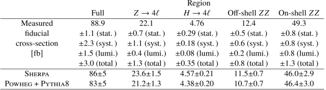
Table 2: Fiducial cross-sections in femtobarns in the full fiducial phase-space and in the following regions of m₄`: Z → 4` (60 <m₄` < 100 GeV), H → 4` (120 < m₄` < 130 GeV), off-shell Z Z(20 < m<sub>4</sub>` <60 GeV or 100 <m_{4`</sub> <120 GeV or 130 <m<sub>4`} <180 GeV) and on-shellZ Z(180 <m<sub>4`</sub> < 2000 GeV), compared to particle-level predictions and their uncertainties as described in Section4. Two predictions are shown with the qq¯→4`process simulated with Sherpa or with Powheg + Pythia8. All other SM processes are the same for the two predictions.

Region

Full Z → 4 ` H → 4 ` Off-shell Z Z On-shell Z Z

Measured 88.9 22.1 4.76 12.4 49.3

fiducial ± 1.1 (stat. ) ± 0.7 (stat. ) ± 0.29 (stat. ) ± 0.5 (stat. ) ± 0.8 (stat. ) cross-section ± 2.3 (syst. ) ± 1.1 (syst. ) ± 0.18 (syst. ) ± 0.6 (syst. ) ± 0.8 (syst. ) [ fb ] ± 1.5 (lumi.) ± 0.4 (lumi.) ± 0.08 (lumi.) ± 0.2 (lumi.) ± 0.8 (lumi.)

± 3.0 (total ) ± 1.3 (total ) ± 0.35 (total ) ± 0.8 (total ) ± 1.3 (total ) Sherpa 86 ± 5 23.6 ± 1.5 4.57 ± 0.21 11.5 ± 0.7 46.0 ± 2.9 Powheg + Pythia8 83 ± 5 21.2 ± 1.3 4.38 ± 0.20 10.7 ± 0.7 46.4 ± 3.0

6 Results

6.1 Measurements

Table 2 gives the measured cross-sections in the full fiducial phase space and in four m

regions, each dominated by different processes from Figure 1, compared to the theoretical predictions described in Section 4. Two predictions are shown, one where the q q ¯ → 4 ` process is simulated with Sherpa at NLO accuracy in QCD and one where it is simulated with Powheg + Pythia8 normalised to a prediction at NNLO accuracy in QCD, as described in Section 4. All the other SM processes are the same in the two predictions. The Sherpa prediction is generally higher than the Powheg + Pythia8 prediction in all but the on-shell region, where the predictions are very close. The agreement between the data and both predictions is generally within the quoted uncertainties. The data central values are above the Powheg + Pythia8 predictions in all regions, and in all but the Z → 4 ` region for Sherpa. In the on-shell region the Sherpa prediction is 1 σ below the data. In Ref. [86] the H → 4 ` cross-section is measured by ATLAS in a slightly different fiducial phase-space to the H → 4 ` region measured here. The phase-space is designed to minimise the contribution from non- H → 4 ` processes. In the dedicated Higgs measurement the cross-section is found to be slightly below the SM prediction. The difference with this measurement is due to the different phase-space cuts, the fact that the non-Higgs processes are subtracted using a data-driven approach, and the fact that a ∼ 1% contribution from Higgs production in association with a b-quark pair is included in the prediction.

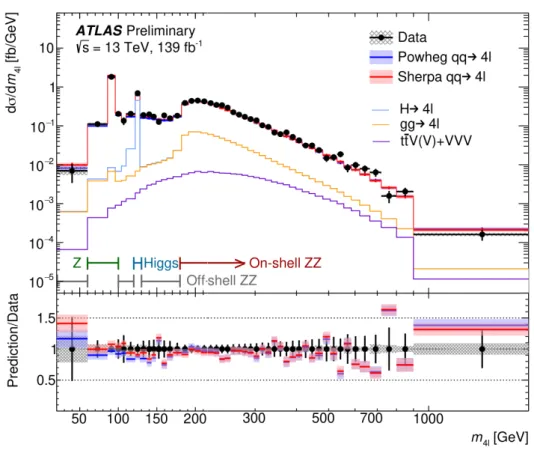
The differential cross-section as a function of m

is shown in Figure 4, in much finer bins than those in Table 2. The breakdown of the contribution from different SM processes is also shown. The features seen in the reconstruction-level distribution are also present here. The SM predictions agree well with the measurement within uncertainties over the entire m

spectrum, with the same features seen as in the comparisons in Table 2.

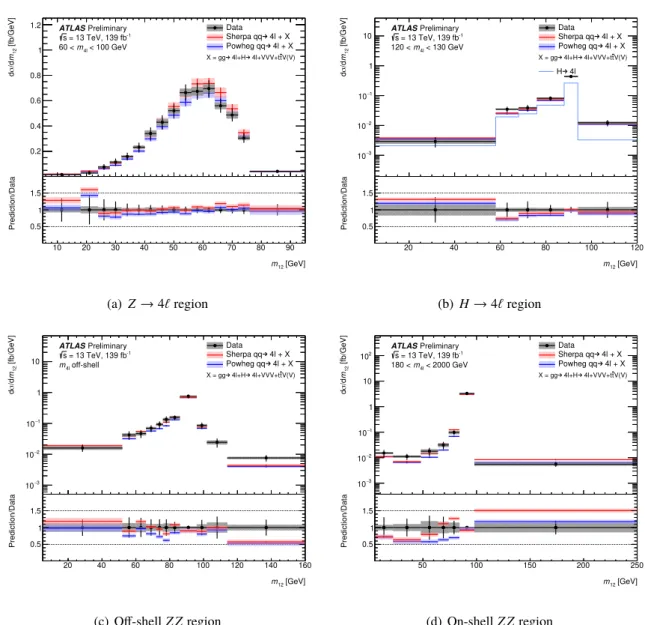
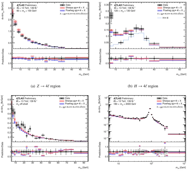
In order to study the different m

regions more closely, Figures 5 and 6 show the cross-section versus

m

and m

respectively in each region. In the H → 4 ` region the contribution from Higgs production is

shown separately. The different regions show peaks in different places due to the kinematic constraints of

Figure 4: Differential cross-section ofm<sub>4`</sub>. The measured data (black points) are compared to the SM prediction using either Sherpa (red with red hashed band for the uncertainty) or Powheg + Pythia8 (blue with blue hashed band for the uncertainty) to model theqq¯→4`contribution. The error bars on the data points give the total uncertainty and the grey hashed band gives the systematic uncertainty. The breakdown of the contribution from different SM processes is also shown in successive stacked histograms. The horizontal lines indicate the boundaries of the different m_{4`</sub>regions in which the other variables are measured. The lower panel shows the ratio of the SM predictions to the data. Thex-axis is on a linear scale untilm<sub>4`} =216 GeV, when it switches to a logarithmic scale.

the m

requirements. For all regions but Z → 4 ` there is a clear enhancement at m

for m

. Conversely, m

only has contributions from on-shell Z bosons in the on-shell region. The Z → 4 ` and off-shell regions are dominated by off-shell photon and Z boson exchange, and the H → 4 ` region is dominated by off-shell Z production. The data are generally well modelled by the SM predictions within uncertainties, apart from m

in the on-shell Z Z region, where the predictions are below the data for m

below m

, and above the data for m

above m

. Here the shapes of the two SM predictions also deviate, indicating differences in the modelling, perhaps related to the modelling of the final-state radiation of photons. The m

and m

measurements provide particular sensitivity to BSM models in which the lepton pairs do not come from Z boson decays, as discussed in Section 6.3.

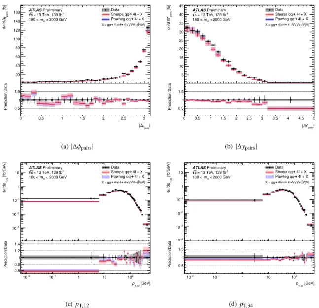
Figure 7 shows the |∆ φ

| , |∆ y

| , p

, and p

differential cross-sections in the highest cross-section on-shell Z Z region. The |∆φ

| distribution peaks at π , with the di-lepton pairs back-to-back. The

|∆ y

| distribution peaks at zero, with a tail going out to five. The p

and p

distributions peak at

around 40 GeV. Overall the SM gives a good description of the kinematics in this region, however the SM

10 20 30 40 50 60 70 80 90 0.2

0.4 0.6 0.8 1 1.2 [fb/GeV]12m/dσd

= 13 TeV, 139 fb-1

s

Preliminary ATLAS

< 100 GeV m4l

60 <

Data 4l + X Sherpa qq→

4l + X Powheg qq→

V(V) t 4l+VVV+t 4l+H→ X = gg→

10 20 30 40 50 60 70 80 90

[GeV]

m12

0.5 1 1.5

Prediction/Data

(a) Z→4`region

20 40 60 80 100 120

3

10− 2

10− 1

10−

1 10

[fb/GeV]12m/dσd 4l→H

= 13 TeV, 139 fb-1

s

Preliminary ATLAS

< 130 GeV m4l

120 <

Data 4l + X Sherpa qq→

4l + X Powheg qq→

V(V) t 4l+VVV+t 4l+H→ X = gg→

20 40 60 80 100 120

[GeV]

m12

0.5 1 1.5

Prediction/Data

(b)H→4`region

20 40 60 80 100 120 140 160

3

10− 2

10− 1

10−

1 10 [fb/GeV]12m/dσd

= 13 TeV, 139 fb-1

s

Preliminary ATLAS

off-shell m4l

Data 4l + X Sherpa qq→

4l + X Powheg qq→

V(V) t 4l+VVV+t 4l+H→ X = gg→

20 40 60 80 100 120 140 160

[GeV]

m12

0.5 1 1.5

Prediction/Data

(c) Off-shellZ Zregion

50 100 150 200 250

3

10− 2

10− 1

10−

1 10 102

[fb/GeV]12m/dσd

= 13 TeV, 139 fb-1

s

Preliminary ATLAS

< 2000 GeV m4l

180 <

Data 4l + X Sherpa qq→

4l + X Powheg qq→

V(V) t 4l+VVV+t 4l+H→ X = gg→

50 100 150 200 250

[GeV]

m12

0.5 1 1.5

Prediction/Data

(d) On-shellZ Zregion

Figure 5: Differential cross-section ofm₁₂in the fourm₄`regions. The measured data (black points) are compared to the SM prediction using either Sherpa (red with red hashed band for the uncertainty) or Powheg + Pythia8 (blue with blue hashed band for the uncertainty) to model theqq¯→4`contribution. In (b) the contribution from Higgs production is shown in addition to the total SM prediction. The error bars on the data points give the total uncertainty and the grey hashed band gives the systematic uncertainty. The lower panel shows the ratio of the SM predictions to the data.

prediction is about 20% lower than the data for 2 . 6 < |∆ y

| < 3 . 2 and 50% lower for |∆ y

| > 3 . 2, indicating a mis-modelling by the simulation in this region of phase-space.

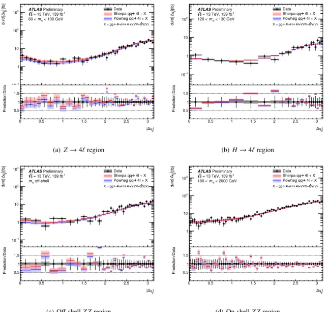
Figure 8 shows the cross-section versus |∆φ

| for each region, where good agreement with the SM prediction is seen. In each region the cross-section peaks when the two leading leptons are back-to-back.

In the Z → 4 ` region this variable is sensitive to electroweak corrections to single- Z production.

Figures 9 and 10 show cos θ

12

and cos θ

34

respectively, in all four regions. These variables are sensitive to

the polarisation of the decaying bosons. A good agreement with the SM prediction is seen in all regions.