s = 13 TeV with the ATLAS Detector Using Multivariate

CERN-THESIS-2017-272 21/08/2017

Technische Universität München Physik-Department

Masterarbeit

Search for top squark Production at the LHC at √

s = 13 TeV with the ATLAS Detector Using Multivariate

Analysis Techniques

von

Jonas Graw München

Freitag, den 18. August 2017

Technische Universität München Physik-Department

Erstgutachter (Themensteller): Prof. Dr. H. Kroha

Zweitgutachter: Prof. Dr. L. Oberauer

I assure the single handed composition of this master’s thesis is only supported by declared resources.

Ich versichere, dass ich diese Masterarbeit selbstständig verfasst und nur die angegebenen Quellen und Hilfsmittel verwendet habe.

München, den 18. August 2017

Unterschrift

Abstract

Supersymmetry is a very promising extension of the Standard Model. It predicts

new heavy particles, which are currently searched for in the ATLAS experiment at

the Large Hadron Collider at a center-of-mass energy of 13 TeV. So far, all searches

for supersymmetric particles use a cut-based signal selection. In this thesis, the use

of multivariate selection techniques, Boosted Decision Trees and Artificial Neural

Networks, is explored for the search for top squarks, the supersymmetric partner of

the top quark. The multivariate methods increase the expected lower limit in the

mass of top squarks by approximately 90 GeV from currently 990 GeV for small

neutralino masses.

Acknowledgments

First of all, I would like to thank Professor Hubert Kroha for giving me the opportunity to study and research in such a fantastic group. I am also very grateful for the proof- reading of my thesis. I greatly benefited from his keen insight.

Secondly, I must express my profound gratitude to Nicolas Köhler and Johannes Junggeburth, who always provided help when I needed some – even at night or on weekends. In addition, I am much obliged to them for proof-reading the thesis. I really enjoyed our time together and I greatly appreciate their unconditional efforts.

Finally, I would also like to express my gratitude to all my friends and my family,

particularly to my mother Regina Graw, for always supporting me.

Contents

Abstract . . . . vii

Acknowledgments . . . . ix

Contents . . . . xi

1 Introduction . . . . 1

2 Theoretical Framework . . . . 3

2.1 The Standard Model of Particle Physics . . . . 3

2.2 Limitations of the Standard model . . . . 6

2.3 Supersymmetry . . . . 6

2.4 The Minimal Supersymmetric Standard Model (MSSM) . . . . 7

2.5 R-Parity . . . . 7

3 The ATLAS Experiment . . . . 11

3.1 The Large Hadron Collider . . . . 11

3.2 The ATLAS Detector . . . . 13

3.2.1 The Inner Detector . . . . 14

3.2.2 The Calorimeter System . . . . 15

3.2.3 The Muon Spectrometer . . . . 16

3.2.4 The Trigger System . . . . 18

4 The search for top squarks . . . . 21

4.1 Reconstruction of physics objects . . . . 21

4.2 Background Processes . . . . 23

4.3 Event Selection . . . . 23

4.4 Monte-Carlo Event Simulation . . . . 26

5 Machine Learning . . . . 29

5.1 Boosted Decision Trees . . . . 29

5.2 Neural Networks . . . . 35

5.3 Overtraining . . . . 38

5.4 Performance Evaluation . . . . 41

6 Analysis . . . . 43

6.1 Input Variables . . . . 43

6.2 Correlations between Input Variables . . . . 47

6.3 Boosted Decision Trees . . . . 51

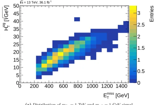
6.3.1 Selection of Signal Samples . . . . 51

6.3.2 Optimization of the Training Configurations . . . . 57

6.3.3 Input Variable Ranking . . . . 67

6.3.4 Final Results . . . . 70

6.4 Neural Networks . . . . 76

6.4.1 Setup . . . . 76

6.4.2 Final Results . . . . 83

7 Summary and Conclusion . . . . 89

Appendix . . . . 91

1 Input Variables . . . . 91

2 Boosted Decision Trees . . . . 95

2.1 Real AdaBoost . . . . 95

2.2 Gradient Boost . . . . 96

2.3 BDT Parameter Plots . . . . 98

3 Neural Networks . . . . 108

3.1 The BFGS algorithm . . . . 108

3.2 Parameter Plots . . . . 109

Bibliography . . . . 119

List of Figures . . . . 125

List of Tables . . . . 133

Chapter 1 Introduction

The Standard Model of particle physics has successfully passed all tests over the last several decades. The last missing particle of the Standard Model, the Higgs boson, was discovered in the ATLAS [1] and CMS [2] experiments at the Large Hadron Collider (LHC) in 2012. There are, however, many experimental and theoretical reasons to believe that the Standard Model is not the final theory of elementary particles. Dark Matter and Dark Energy, established by astrophysical observations, dominate the energy content of the universe and cannot be explained by the Standard Model [3, 4]. The smallness of the Higgs boson mass compared to the energy scale of the unification of all interaction strengths requires an explanation, the so-called naturalism or fine-tuning problem of the Higgs mass in the Standard Model.

Supersymmetry is a very promising extension of the Standard Model, in which every Standard Model particle is accompanied by a supersymmetric partner particle differing by spin

. The searches for supersymmetric particles like the top squark – the partner of the top quark – have been performed with cut-based signal selection methods in the ATLAS experiment up to now. In this thesis, a search for top squarks with ATLAS at 13 TeV centre of mass energy has been performed using machine learning or multivariate methods which allow for the efficient combination of many partially correlated discriminating variables.

In Chapter 2, the Standard Model and supersymmetry are introduced, while in Chapter 3 the Large Hadron Collider and the ATLAS Experiment are described.

Chapter 4 explains the signatures of top squark production in ATLAS and the cut-

based search as a reference. Chapter 5 introduces the machine learning methods used,

Boosted Decision Trees (BDT) and Artificial Neural Network (ANN). Chapter 6

finally describes the results of the multivariate signal selection techniques for the top

squark search. The summary of the analysis and results are given in Chapter 7.

Chapter 2

Theoretical Framework

2.1 The Standard Model of Particle Physics

The particle content of the Standard Model is shown in Figure 2.1. Besides the three generations of quarks and leptons, the matter particles with spin

, there are force mediators with spin 1 and the scalar Higgs boson.

Four fundamental forces are known – the strong, the weak, the electromagnetic and the gravitational force. All fundamental forces, except gravitational, are described by the Standard Model (SM based on the gauge symmetry groups [5, 6]

SU (3)

⊗ SU (2)

⊗ U (1)

. (2.1) The gauge symmetries predict mediators of the interactions with spin 1, called gauge bosons. SU(3)

is the gauge group describing the strong force with eight gluons as force carriers, whereas SU (2)

⊗ U (1)

is the gauge group of the unified electroweak interaction. SU (2)

is the gauge group of the weak force with three force carriers W

, i = 1, 2, 3, belonging to the weak isospin outer components T

as charge operators.

U (1)

is the symmetry group of the weak hypercharge Y , which is related to the electric charge Q and T

via

Q = T

+ Y

2 (2.2)

and is mediated by a gauge boson B.

The electroweak gauge bosons mix to the electrically charged mass eigenstates.

W

= 1

√ 2 · W

∓ iW

, (2.3)

and to neutral mass eigenstates Z

A

=

cos θ

− sin θ

sin θ

cos θ

· W

B

, (2.4)

Figure 2.1: Particles of the Standard Model [7].

2.1 The Standard Model of Particle Physics

where Z

is the mediator of the neutral weak interaction and heavy partner of the photon field A. The Weinberg mixing angle θ

is related to the gauge coupling constants corresponding to the hypercharge, g

and g

of the weak hypercharge and the weak isospin interaction via

tan θ

= g

g

. (2.5)

The SU (3)

color gauge interaction predicts the existence of eight gluons as carriers of the strong force coupling to the quarks which all appear in three color states [8].

The gauge symmetries predict invariance of the theory under local phase transforma- tions of the matter fields and the massless spin 1 gauge bosons. The problem that the gauge bosons of the weak interaction are massless in contradiction to experimental observations was solved by introducing spontaneous weak interaction breaking of the electroweak gauge symmetry [9–11], which, in its minimal form requires a complex scalar weak isospin doublet Φ with Y = 1. The potential of the scalar field

V (φ) = µ|φ|

+ λ|φ|

. (2.6) acquires a non-zero vacuum expectation value

Φ

= r −µ

2λ (2.7)

for negative parameter µ such that the ground vacuum state violates the SU (2)

⊗ U (1)

gauge symmetry. The spontaneous symmetry breaking leads to masses for the weak W

and the Z

, while the photon field A remains massless corresponding to the unbroken U (1) gauge group of the electromagnetic interaction. A further consequence is the existence of a new scalar particle, the Higgs boson. It was discovered by ATLAS and CMS experiments of the LHC in 2012 [1, 2] with a mass of about 125 GeV. All measured properties so far fit the Standard Model predictions [12–16].

The spin

particles in the SM comprise six quarks with electric charges

e or −

e and six leptons which obtain their mass via Yukawa interactions with the Higgs field [8]. The Yukawa couplings are proportional to the fermion masses. Neutrinos may have additional mass terms.

The left-handed states of the quark and the leptons are doublets of the SU (2)

weak interaction gauge symmetry,

u d

L

, c

s

L

t b

L

, (2.8)

ν

e

L

, ν

µ

L

, ν

τ

L

, (2.9)

and participate in the charged weak interaction via the exchange of W

bosons and transition from up to down states and vice versa.

Right-handed quarks and right-handed leptons have isospin T = 0 and are singlets of the SU (2)

symmetry, i. e. they do not participate in the charged weak interaction.

2.2 Limitations of the Standard model

Despite the greatness of the SM passing all experimental tests with high precision, there is a large number of open questions which show that the Standard Model (SM) cannot be complete.

The SM does not allow for neutrino oscillations [17–19] as neutrinos are massless in the SM.

From astrophysical and cosmological observations it is known that only 4.9% of the universe consists of SM particles, whereas 26.8% is so-called Dark Matter and the remaining fraction Dark Energy, neither of which is described in the SM [3, 4]. It also appears that the matter-anti-matter asymmetry in the universe cannot be explained by the Standard Model.

Another problem – and one of the key arguments for supersymmetry – is the naturalness- and, related, hierarchy-problem. The question is, why the electroweak scale (≈ 100 GeV) is so much smaller than the Planck-scale (10

GeV) [20]. Since the quantum loop corrections to the Higgs boson mass diverge quadratically with the cutoff scale, it remains unnatural fine-tuning of the SM parameters to keep the Higgs boson mass as low as 125 GeV.

Finally, the SM does not describe (quantum) gravity. One very promising extension of SM which solves several problems is supersymmetry.

2.3 Supersymmetry

Supersymmetry (SUSY) transforms boson into fermion states and vice versa.

As a consequence, in supersymmetric extensions of the SM, there is a supersymmetric partner, each SM particle which differs by spin

, but otherwise has the same mass as its super-partner. In this case, fermionic and bosonic loop corrections to the Higgs mass would exactly cancel, solving the naturalness problem of to the Higgs mass.

SUSY, however, has to be a broken symmetry, since no super-partners of the SM

particles with the same mass have been observed. In order to solve the naturalness

2.4 The Minimal Supersymmetric Standard Model (MSSM)

problem, the SUSY breaking scale must not be higher than a few TeV, which could be within the reach of the LHC, in particular, the masses of the partners of the top quark.

2.4 The Minimal Supersymmetric Standard Model (MSSM)

The MSSM is the minimal supersymmetric extension of the SM with the smallest number of additional particles of the MSSM. The particles of the MSSM are shown in Figure 2.2. Instead of one Higgs doublet, two Higgs doublets are required, one for up- type and one for down-type fermions in order to avoid gauge anomalies. Spontaneous electroweak symmetry breaking in this case leads to five Higgs bosons: a Standard Model-like h, another heavier neutral scalar boson H

, a pseudo-scalar neutral boson A and two charged Higgs bosons H

.

Each of these bosons is provided with its own superpartner. The nomenclature is as follows: The supersymmetric partners of bosons are denoted by an -ino ending, the five Higgsinos and the gauginos, the three Winos, the Bino, the eight gluinos and the photino. The supersymmetric partners of the SM fermions are denoted by an s- at the beginning, squarks and sleptons as the partners of the quarks and the leptons. The symbols of the supersymmetric particles are marked with a tilde on the SM particles symbols, e. g. ˜ t for a top squark. The spin-

Higgsinos, Binos and Winos mix to four neutral mass eigenstates χ

, i = 1, ..., 4, the neutralinos, and four charged mass eigenstates χ

, i+1, 2, the charginos. Since right-handed and left-handed SM fermions couple differently to the weak interaction, the two charginos are distinguished for each SM fermion with mass coupling scalar superpartner states e l

and q e

for sleptons and squarks, respectively.

2.5 R-Parity

As the lepton and baryon number are not conserved in SUSY theories, the proton is allowed to decay rapidly without an extra symmetry, which prevents it.

In the MSSM, a new conserved quantum number is introduced, the so-called R-parity

P

= (−1)

(2.10)

where B is the baryon number, L the lepton number and S the spin of the particle.

The R-parity is 1 for SM particles and −1 for supersymmetric particles. In this

quarks

u c t

d s b

e µ τ

ν _e ν _µ ν _τ

leptons

gauge bosons

Higgs bosons γ h, H ⁰

Z A

W ^± H ^±

g

squarks

˜

u _1,2 c ˜ _1,2 t ˜ _1,2

d ˜ _1,2 s ˜ _1,2 ˜ b _1,2

˜

e _1,2 µ ˜ _1,2 τ ˜ _1,2

˜

ν _e ν ˜ _µ ν ˜ _τ

sleptons gauginos

˜

χ ⁰ ₁ χ ˜ ⁰ ₂

˜

χ ⁰ ₃ χ ˜ ⁰ ₄

˜

χ ^± ₁ χ ˜ ^± ₂

˜ g

Figure 2.2: Particles of the Minimal Supersymmetric Standard Model [21].

2.5 R-Parity

thesis, any SUSY model with R-parity conservation is considered. In this case, the lightest supersymmetric particle (LSP) is stable, and super-partners are produced in pairs from SM particle collisions. If the LSP is neutral and only weakly-interacting, it proves to be an excellent candidate for a Dark Matter particle. The lightest neutralino,

˜

χ

, is often assumed to be the LSP. In SUSY models with R-parity violation, other

symmetries are introduced to prevent rapid proton decay.

Chapter 3

The ATLAS Experiment

3.1 The Large Hadron Collider

The Large Hadron Collider (LHC) at CERN, the European centre for particle physics near Geneva, collides protons cylindrically at a centre-of-mass energy of 13 TeV and a luminosity of L = 1.5 · 10

cm

s

.

It is located in a tunnel at a depth between 50m and 175m underground and has a circumference of about 26.6 km.

The LHC utilizes 1232 superconducting dipole magnets to keep the protons on their circular path. They are operated at a maximum current of 12 kA resulting in a magnetic field of 8.3 T. The proton beams consist of 2808 bunches of 10

protons each. The bunch spacing time is 25 ns.

Before injection into the LHC, the protons are pre-accelerated in several other accel- erators: First a linear accelerator, then the proton synchrotron (PS) and finally the Super Proton Synchrotron (SPS), which increases the proton energy to the injection energy of 450 GeV. Figure 3.1 shows the CERN accelerator complex schematically.

There are four detectors at the LHC: ATLAS (A Toroidal LHC ApparatuS) and CMS (Compact Muon Solenoid), which are designed to search for production and decays of the Higgs boson and for signatures of physics beyond SM, LHCb (Large Hadron Collider beauty detector), a bottom quark physics experiment and ALICE (A Large Ion Collider Experiment), built for the investigation of heavy ion collisions.

The main goal and greatest success of the LHC so far was the discovery of the Higgs

boson in 2012 by the ATLAS [1] and CMS [2] experiments.

Figure 3.1: Schematic layout of the CERN accelerator complex [22].

3.2 The ATLAS Detector

3.2 The ATLAS Detector

ATLAS [23] is one of the two main experiments at the LHC, along with the CMS detector. It has a length of 46 m, a diameter of 25 m and a mass of 7000 tons. It is located about 100 m underground.

Figure 3.2 shows the ATLAS Detector and its main components. Like other collider detectors, it consists of a barrel region containing co-axial cylindric detector layers and endcaps with two disk-shaped detector layers. Figure 3.3 explains the functionality of the sub-detectors for the identification and measurement of various particle types.

Figure 3.2: Schematic views of the ATLAS detector [23].

ATLAS uses a right-handed coordinate system of which the origin cuts the nominal interaction point. The z-axis is the proton beam axis, whereas the x-axis points towards the centre of the LHC ring. The x-y-plane is the transverse plane with respect to the proton beam. To describe points in the detector, spherical coordinates (r, θ, φ) are used, where r is the distance from the origin, θ the polar angle and Φ the

azimuthal angle in the x-y-plane.

Alternatively, the pseudo-rapidity η = −ln tan

serves to describe particle pro-

duction in the r-z-plane. It is related to the transverse momentum p

and the transver-

sal energy E

of particles relative to the beam axis by the expressions p

=

q

p

+ p

= |p|

cosh (η) , (3.1)

E

= E

cosh (η) . (3.2)

Figure 3.3: Schematic illustration of the detection of particles in the ATLAS detector components [24].

3.2.1 The Inner Detector

The Inner Detector, depicted in Figure 3.4, is the innermost detector component,

which consists of three layers: the Pixel Detector, the Semiconductor Tracker and

3.2 The ATLAS Detector

the Transition Radiation Tracker. The Inner Detector is surrounded by a 2T super- conducting solenoid magnet in order to measure the deflection and momentum of charged particles up to a pseudo-rapidity of |η| =2.5.

The Pixel Detector is the detector closest to the beamline. Its purpose is to reconstruct interaction and decay vertices. It consists of silicon pixel sensors with 80 million pixels in total and a spatial resolution of 14 µm in the transverse plane and 115 µm in the direction of the beam axis which are arranged in three layers in the barrel region and three disks in the end-caps. The innermost layer is called B-layer, since it is particularly important for the tagging of b-quark jets making use of the long lifetime and decay length of B hadrons.

The Semiconductor Tracker is built around the Pixel Detector, consisting of four layers and nine disks of silicon microstrip detectors with a resolution of 17 µm and 580 µm in transverse and in longitudinal direction respectively.

The outermost layer of the Inner Detector is the Transition Radiation Tracker, which also helps to identify electrons. It consists of straw drift tubes with a diameter of 4 mm, which are filled with a gas mixture of Xenon (70%) and carbon dioxide (27%).

It measures the particle tracks in the transverse plane with about 30 layers of straw tubes with a resolution of 130 µm. Electrons are distinguished by measuring the transition radiation emitted when they traverse carbon foils inserted between the straw tube layers.

3.2.2 The Calorimeter System

The Calorimeter System (illustrated in Figure 3.5) surrounds the Inner Detector and measures the energy of particles interacting electromagnetically or hadronically. There are two main parts – the electromagnetic calorimeter and the hadronic calorimeter.

Both consist of metal absorber plates interleaved between active detector material, liquid argon in the electromagnetic and hadronic endcap calorimeters and scintillating plastic tiles in the barrel hadronic calorimeter.

The electromagnetic calorimeter, consisting of a barrel and an endcap part, is located in the front and measures the energy of electrons and photons. The barrel part covers |η| < 1.475, whereas the end-caps cover 1.375 < |η| < 2.5. Copper plates are used as absorber material. Electromagnetic showers start in the copper plates.

The shower particles ionize the Argon atoms in the active groups. The ionization electrons are collected on electrode boards in the liquid Argon gaps. The thickness of the electromagnetic calorimeter is more than 20 radiation lengths, such that photons and electrons are completely absorbed.

The hadronic calorimeter surrounds the electromagnetic calorimeter and captures

Figure 3.4:The ATLAS Inner Detector [23].

hadrons traversing the electromagnetic calorimeter. It covers the range |η| < 4.9 and consists of three different components: The Tile Calorimeter utilizes steel absorber plates and scintillating tiles as active material covering |η| < 1.7, whereas the hadronic endcap calorimeter uses copper absorber plates and liquid argon as active material in the range 1.5 < |η| < 3.2. The forward liquid-argon calorimeter consists of three layers with tungsten absorber plates and covers 3.1 < |η| < 4.5. The thickness of the hadronic calorimeter is greater than 10 radiation lengths in order to absorb all hadrons.

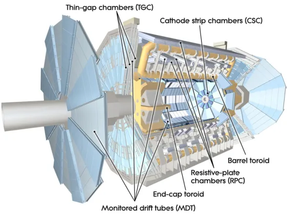
3.2.3 The Muon Spectrometer

Apart from neutrinos, muons are the only Standard Model particles, that pass the calorimeters. The Muon Spectrometer (shown in Figure 3.6) is the outermost and by far the largest component of the detector. It uses a toroidal magnetic field of 0.5 to 1 T to bend the muon tracks. Its pseudo-rapidity range is divided into three regions:

The barrel part covers the region |η| ≤ 1.0, while the regions 1.4 ≤ |η| ≤ 2.7 are

3.2 The ATLAS Detector

Figure 3.5: The ATLAS Calorimeter System [23].

covered by two separate endcap magnets. The η regions in between are covered by both magnet systems.

Two different kinds of muon chambers are used: Precision tracking chambers and trigger chambers. The precision muon tracking chambers allow for very precise mea- surement of the momenta of muons. The momentum resolution for 1 TeV muons is 10%, dominated by the chamber position resolution of 35 µm and the chamber alignment accuracy of 30 µm, while it is 3-4% for 100 GeV muons. Multiple scattering starts to become relevant. Two types of tracking chambers are used:

The Monitored Drift Tube chambers (MDT) consist of aluminium drift tubes of 30 mm diameter filled with a gas mixture of Argon (93%) and carbon dioxide (7%) at 3 bar pressure. Since there are higher background rates of neutrons and γ-rays close to the beamline, Cathode Strip Chambers (CSC), operated with Argon (30%), carbon dioxide (50%) and tetrafluoromethane CF

(20%), are used in the very forward regions of the inner end-caps wheels.

Two types of muon trigger chambers are made use of: Resistive Plate Chambers

(RPC), in the barrel region (|η| <1.05) and Thin Gap Chambers (TGC) in the end-

Figure 3.6: The ATLAS Muon Spectrometer with eight barrel toroid coils and two endcap toroid magnets in separate cryostats. The muon chambers are installed on the barrel toroid coils or on separate wheel-shaped support structures in the end-cap [23].

cap regions (1.05< |η| <2.4). The trigger chambers have a poorer spatial resolution than the tracking chambers but provide fast signals for the muon trigger and for the determination of the proton bunch collision time that the muon belongs to.

3.2.4 The Trigger System

At the LHC, proton bunch collisions take place at a frequency of 40 MHz. A collision event contains about 1 MB of information. The resulting data rate would be much too high to be recorded. Therefore, the data rate is drastically reduced by a two-stage trigger system down to a maximum recording rate of 1 kHz [25]. The trigger scheme is presented in Figure 3.7.

The first trigger stage (level-1 trigger) is completely hardware-based and uses the

transverse momentum p

, the missing transverse energy E

and the energy of

3.2 The ATLAS Detector

Figure 3.7: Schematics of the ATLAS trigger system [25].

hadron jets to reject events and define regions of interest (RoI) for evaluation by the next trigger stage.

The second trigger stage is called High-Level Trigger (HLT) and is software-based. It

utilizes simplified versions of the reconstruction algorithms used by ATLAS for the

measurement of particle and event properties.

Chapter 4

The search for top squarks

In this thesis, the search for t-quarks is examined by using multivariate analysis ˜ techniques. The considered model together with the final state is presented in this chapter. This is followed by a short introduction of physical objects, by analyzing the different background events and by describing the Monte-Carlo event generation.

Figure 4.1 depicts a sketch of the simplified ˜ t

-model used throughout this thesis.

The t ˜

is assumed to be produced pairwise in the pp-collisions. Each ˜ t

then decays into a fully hadronically decaying top and in χ ˜

, which is assumed to be stable and to leave the detector system undetected. So the final state of interest consists of six jets, two of which are b-tagged, and a large amount of E

. The masses of the two sparticles are considered to be the only free parameters of the model, while all remaining sparticles are decoupled.

4.1 Reconstruction of physics objects

The physics objects considered here are jets, electrons, muons and the missing trans- verse energy. Hadronic τ lepton are identified from jets using substructure informa- tion [27].

The primary interaction vertex reconstruction uses charged particle tracks reconstruc- tion in the Inner Detector [28]. Events are required to obtain at least one vertex with at least two well reconstructed tracks [29]. Well-reconstructed tracks are required to have a transverse momentum p

>400 MeV and a pseudo-rapidity |η| <2.5. The primary interaction vertex is defined as the vertex with a maximum P

p

of the associated tracks. The remaining reconstructed vertices are called pileup vertices.

The anti-k

algorithm [30] with a radius parameter of R = 0.4 is employed to re- construct jets starting from topological clusters [31]. Area-based corrections using calorimeter information are performed for contributions from pileup interactions [32].

Vertex reconstruction of b-hadron decays is an important ingredient for b-tagging,

˜ t

˜ t

t W

t W

p p

˜ χ ⁰ ₁

b q

q

˜ χ ⁰ ₁

b

q q

Figure 4.1: Sketch of pair production of top squarks with fully-hadronic decay into final states withb-quark jets of which two are fromb-quarks and missing energy due to the lightest super-symmetric particleχ˜⁰₁leaving the detector undetected [26].

the identification of b-quark jets. Since b-hadrons have a long lifetime (some more than 1 ps [33]), it is possible to distinguish between b-jets and jets from lighter quarks or gluons. Multivariate methods, neural networks and Boosted Decision Trees (BDT), are used in order to collect the maximum information for b-tagging [34]. A jet is b-tagged if it satisfies the 77% selection efficiency working point at a misclassification rate of less than 1% for light jets [35]. Both numbers are extracted from simulated t ¯ t-events.

Electrons are reconstructed in the range |η| < 2.47 and p

> 7 GeV using energy deposit in the electromagnetic calorimeter matching a track in the Inner Detector in energy and direction [36]. Likelihood-based multivariate identification techniques are applied to discriminate electrons from jets. Electron candidates that satisfy the Loose LH selection criteria are selected if there is not any jet in the cone 0.2 < ∆R < 0.4 or a b-jet within ∆R < 0.2. Light jets within ∆R < 0.2 are discarded as electrons.

The electromagnetic showers of electrons are distinguished from the ones of hadron jets by a likelihood-based method. A reconstructed jet is taken as an electron if

∆R = q

(η

− η

)

+ (φ

− φ

)

< 0.2. (4.1)

If the jet is b-tagged, it is always kept, and the electron is discarded.

4.2 Background Processes

Both the Inner Detector and the Muon Spectrometer are used to reconstruct muons in the range |η| < 2.7 and p

> 6 GeV. The Inner Detector and Muon Spectrometer tracks are combined into one single track forming the muon. The ∆R separation between a muon and a nearby jet must be greater than 0.4, in order to keep the muon.

Otherwise, the jet is kept.

The missing transverse momentum p

is the negative sum of the transverse mo- menta of all reconstructed physics objects in an event. Since neutrinos and other only weakly interacting particles are not detected by any elements of the detector, they lead to missing transverse momentum. The magnitude of p

is the missing trans- verse energy E

. High E

is an important criterium in the search for processes beyond the Standard Model.

4.2 Background Processes

Most of the SM background in the 0` channel arises from t t ¯ where one top quark decays hadronically and the other one leptonically. The produced lepton from the decay is not reconstructed, and the neutrino leads to an amount of E

after preselection comes from t ¯ t, where top quarks are produced, which decay into a W -boson and a b-quark each, where the W -boson decays either into two quarks, or into a lepton and a neutrino with the lepton either being falsely classified as a jet through a hadronic decay (τ ) or not being reconstructed (e, µ) leading to E

. The second largest background arises from the production of a Z-boson with heavy jets, where the Z -Boson decays into two neutrinos Z → ν ν, leading to very high ¯ E

. Another important background process is the production of a W -boson in combination with heavy jets, where the W -boson mostly decays via W → `ν, and the lepton escapes directly. Further background processes are single top quark production in combination with at least one jet. In comparison to t t, single top quarks are produced weakly and ¯ were discovered at the Fermilab Tevatron Collider in 2009 [37, 38]. The production of t t ¯ + Z where the Z-boson decays into neutrinos also contributes to the final states.

Processes involving a pair of two bosons, also known as diboson, are rare, as well as t t ¯ + W processes. Single Photon and ttγ processes are negligible [26].

4.3 Event Selection

In order to search for top squark ˜ t

decays, signal regions (SR) are defined [26] by

cuts which suppress the SM background while keeping the signal events with high

efficiency. Two signal regions are used to search for high top squarks masses: signal

region A (SRA) for the case of large mass differences ∆m(˜ t

, χ ˜

) between top squarks and the neutralinos χ ˜

and signal region B (SRB) for smaller, intermediate mass differences ∆m(˜ t

, χ ˜

). SRA is optimized for m

1

=1 TeV and m

1

= 1 GeV, SRB for m

= 600 GeV and m

1

= 300 GeV.

Both signal regions have the following preselection in common: A missing transverse momentum trigger is required which is fully efficient for offline calibrated missing transverse energies E

> 250 GeV. Thus, a cut on E

> 250 GeV is applied. In addition, at least four jets are required, where the transverse momenta of the two most energetic ones must be at least 80 GeV, while the third and forth jet have to have transverse momenta greater than 40 GeV. In addition, two of the b-tagged jets are required to have a b-tag. This preselection is also the starting point for all studies presented in the thesis.

Events with wrongly measured E

, due to multijet, arising from mismeasured jets, will be rejected by requiring the difference between the azimuthal angles

∆φ jet

, p p p

of the three highest p

jets and the missing transverse mo- mentum vector p

to be greater than 0.4.

The track transverse momentum p

is defined as the sum of the transverse mo- menta of all ID-tracks belonging to the primary vertex. The corresponding missing track transverse momentum and energy are denoted by p

and E

. It is required that E

> 30 GeV and

∆φ

p p

p

, p p p

< π

3 . (4.2)

Depending on the boost of the decay products, sometimes the six jets with a radius parameter R = 0.4 are either all reconstructed individually or if two jets are a distance R of less than 2R apart from each, some of the jets merge. In the latter case, hadronic top decays must be reconstructed by the anti-k

-clustering algorithm with R = 0.8 or R = 1.2 reclustering. For high top squark masses, two R = 1.2 jets (with mass m

and m

) and at least one top-candidate, i. e. m

> 120 GeV, are required. Three different regions are defined: one (TT) with a second top candidate (m

>120 GeV), one (TW) without a second top candidate but with a W candidate (60 GeV< m

< 120 GeV), and one (T0) where the second jet is not even a W candidate (m

< 60 GeV). Each region has different optimized selection cuts and signal-to-background-ratios in t ¯ t-events.

Since the neutralinos χ ˜

are undetectable, the missing transverse energy is a highly important discriminating variable. Therefore, background events with semi-leptonic t t ¯ decays, where the lepton is not reconstructed, are rejected by requiring the transverse mass m

=

q

E

− p

of p

and the b-tagged jet with minimal azimuthal

4.3 Event Selection

distance to p

to be m

=

q

2p

E

1 − cos

∆φ p p p

, p p p

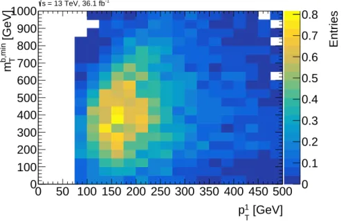
> 200 GeV. (4.3) As shown in Figure 4.2, the majority of t t ¯ events is rejected by this requirement while minor proportions of the two signal models are rejected.

Figure 4.2:m^b,min_T distribution for signal (purple and orange dashed and dotted lines) and background (histograms) events after preselection and one further cutm^b,min_T >50GeV.tt¯ will be surpressed [26].

The following selection criteria are used for signal region A only: The mass m

of the leading R = 0.8 reclustered jet must be greater than 60 GeV. It can be interpreted as a W candidate.

The transverse momentum of an individual neutralino cannot be evaluated, since

there are two of them. The stransverse mass m

is defined by [39]:

m

= min

q₁+q₂=p^miss_T

h max{m

p p p

, qq q

, m

p p p

, qq q

} i

, (4.4)

where two the transverse momenta of top-candidates are denoted by p

and p

. Two methods have been used to form a top quark candidate, a χ

and a ∆R

based method. In both cases, the two b-jets with the highest b-tagging BDT-score are taken as b-jets b

and b

when forming the top candidates. The remaining jets are regarded as light quark jets. In the case of the χ

method, χ

=

2

mtrue

is minimized by using all pairs of light quark jets and m

=80.4 GeV (W -boson mass). The two W candidates with minimal χ

are then combined with b

and b

jets to form top candidates by minimizing χ

=

true

with m

= 172 GeV (top quark mass). The ∆R

method employs ∆φ in the transverse plane instead of χ

to find the W candidates. The masses of the top candidates obtained by the ∆R

method are denoted by m

and m

. The top candidates going into the stransverse mass calculation are the ones from the χ

method. Events with a transverse mass of m

<400 (500) GeV respectively are discarded. The ∆R

candidates are used in another signal region not described.

For signal region B, m

is constructed additionally from the b-jet farest away from p

. Table 4.1 summarizes all cuts.

Figure 4.3 shows the 95% CL upper limits on the ˜ t

˜ t

production cross section decay branching as a function of the top squark and neutralino mass for the cut-based signal selection described above. The solid red line depicts the observed limits. The area below it is excluded at 95% confidence level. The question analyzed in this thesis is whether these limits can be improved with the help of multivariate analysis methods.

4.4 Monte-Carlo Event Simulation

In order to search for supersymmetric particles, it is necessary to simulate them.

Signal models are generated with MadGraph5_aMC@NLO [40], PYTHIA8 [41] and

EvtGen [42] v.1.2.0. The matrix elements are calculated at tree level and matched

with the parton showering via the CKKW-L prescription [43]. In order to generate

the signal samples, the parton distribution function set NNPDF2.3LO [44] is used

together with the A14 fine-tuning parameter set [45]. Cross-sections calculations are

based on next-to-leading order logarithmic accuracy, matched to next-to-leading order

supersymmetric QCD [46–48], which might also serve for possible future accelera-

tors [49].

4.4 Monte-Carlo Event Simulation

Figure 4.3: Exclusion limits in the ˜t₁−χ˜⁰₁ mass plane with the cut method for signal selection [26].

Table 4.1:Selection criteria for SRA and SRB [26]

Signal Region TT TW T0

m

> 120 GeV

m

> 120 GeV [60, 120] GeV < 60 GeV

m

> 200 GeV

N

≥ 2

τ -veto yes

∆φ jet

, p p p

> 0.4

A

m

> 60 GeV

∆R (b, b) > 1 -

m

> 400 GeV > 400 GeV > 500 GeV E

> 400 GeV > 500 GeV > 550 GeV

B m

> 200 GeV

∆R (b, b) > 1.2

Likewise, simulated events are used for the description of the SM background pro- cesses. Top-quark pair production, where at least one of the top quarks decays into a lepton and the single top production are simulated with POWHEG-Boxv.2 [50] and PYTHIA6 [51] with the CT10 PDF set [52] and the Perugia set [53]. Z+ jets and W + jets are generated with SHERPAv2.2.1 [54] and the NNPDF3.ONLNLO [42]

set. MadGraph 5_a MC@NLO [40] and PYTHIA8 [41] generate t t ¯ + V and t ¯ t + γ samples with NNPDF3.0NLO [55], for which NNPDF2.3LO [44] with the A14-set [45]

is used. SHERPAv2.2.1 [54] and the CT10 [52] set generate diboson samples, whereas SHERPAv2.1 [54] and the CT10 set [52] generate V γ samples.

The detector simulation [56] is performed using GEANT4 [57]. The simulation of

the calorimeter response can be achieved with a full or a fast simulation [58]. Events

involving the interaction of more than one proton pair are generated with the MSTW

2008 [59] and the A2 set [60].

Chapter 5

Machine Learning

In this thesis, the possibility of increasing the signal significance is investigated by using machine learning algorithms for the search for top squarks in the full hadronic decay channel using simulated signal and background events. The Monte Carlos (MC) events are split into two halves: One half is used to train the algorithms (training sample) and the other half serves to apply the event selection to (test sample). After training with MC simulated events, the algorithm can also be applied to the data.

For the analysis, the TMVA (Toolkit for Multivariate Data Analysis with ROOT) program package [61] was employed.

5.1 Boosted Decision Trees

One widely-used machine learning method is the Boosted Decision Trees (BDT) [61].

A decision tree is illustrated in Figure 5.1. It is a binary tree consisting of nodes at which the data are divided into two subsets, a signal-like and a background-like subset. Variables are used, which separate best at the node. The purity p =

gives the fraction of signal events at the node.

Before determining the optimum cuts for the top squark search, N

grid points are chosen for each of the N

input variable, picked at equal distance: A variable var

(j = 1, ..., N

) is selected for which the maximum value of the training sample is var

, whereas the corresponding minimum is denoted by var

. Then the grid points var

with i = 1, ..., N

are determined by

var

= var

+

var

− var

· i

n

+ 1 . (5.1)

For illustration, a single variable is assumed, e. g. the missing transverse energy E

with a maximum value of 1000 GeV and a minimum value of 200 GeV. For three grid

points, E

=400 GeV, E

=600 GeV and E

=800 GeV define the possible

cut values.

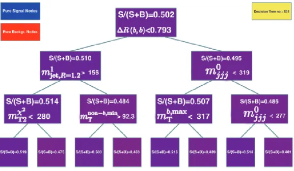
Figure 5.1: Example of the training of an initial decision tree for the top squark search chosen. The colors visualize the signal purity p= _S+B^S . The blue color stands for a pure signal sample withp= 1and red for a pure backgroundp= 0. The colors illustrate the local purity of the node. The bluer, the larger the signal fraction.

For each variable n

many possible cuts are received. The question arises which variables and which cut values are optimal. As a criterion, the best signal purity p

p = S

S + B (5.2)

is used along with the so-called Gini-Index p · (1 − p). The index has its maximum at p = 0.5 and is symmetric with respect to it, meaning that it does not distinguish between the case of M signal and N background events and the case of N signal and M background events. For p = 0 and p = 1 the Gini index equals zero. The smaller the Gini index, the greater the excess of either signal or background. In order to decide which variable and which cut value to use, the sum of the two Gini Indices for the signal-like region and the complementary background-like region of each variable and of each cut value is taken, being weighted by the relative fraction of events (in the following just called Gini index)

G = w

· p

· (1 − p

) + w

· p

· (1 − p

) = N

N

· S

· B

N

+ N

N

· S

· B

N

, (5.3)

which is calculated for each variable and each cut value. Here N

= S

+ B

is the

5.1 Boosted Decision Trees

total number of (weighted) events in node i, and N

= N

+ N

is the total number of (weighted) events in the mother node. Equation 5.3 can be simplified:

G = w

· p

· (1 − p

) + w

· p

· (1 − p

) = 1 N

·

S

· B

N

+ S

· B

N

(5.4) By minimizing Equation 5.4, the so-called separation gain S is maximized:

S = p

· (1 − p

) − G (5.5)

Here, p

is the purity of the mother node. In order to determine the Gini indices for E

at a cut value of 600 GeV, the Gini Indices for E

<600 GeV and for E

≥600 GeV are calculated and added together. The variable and the cut value are chosen for which the Gini index is minimal compared to all other choices.

The cut giving best separation in the first node at the initial tree is E

≤ 453 GeV for the exemplary training. Events satisfying the labeled condition E

<453 GeV in Figure 5.1 are piped to the right node in the chosen scheme of this thesis. The right node, fulfilling the cut condition, is also called ”true” branch. The right branch is the more background-like event branch and the left one is the more signal-like branch, which means that the purity of the right branch p

is smaller than the purity of the left branch: p

≤ p

.

More than 90% of the events in the left branch are signal events (purity p = 0.901).

This node does not split further due to the hypothetical new background-like node being smaller than the minimal node size allows. The minimal node size will be discussed in the next paragraph. The right node has a signal contamination of 25%.

These events are further separated using the next best discriminating variable, in this case m

with a separation edge of 364 GeV. The best discriminating variable cut of the remaining events is m

< 364 GeV. The subsequent right side node has a purity p = 0.187 and does not split further. The left side node splits once more for the cut m

<176 GeV, resulting in purities of p = 0.772 and p = 0.334 respectively. When the events at the final split are looked at, then events located on the left side are classified as signal events (and should have a purity p > 0.5, whereas the events on the right side are classified as background events (and should have a purity p ≤ 0.5).

If the number of nodes were not constrained, a purity of either 0 or 1 would mostly

be the case for the final nodes. The problem of such training is then that the tree

essentially memorizes each event in the training sample individually. This situation

is called overtraining. The events, not being trained with (test samples) have a

much worse score. Therefore, the amount of branchings needs to be limited. Several

parameters control when a node will not be split further. The parameter maximal

depth defines the maximal number of branchings. The default value is three, which

means that the events can be split three times at most until reaching the final node, as depicted in Figure 5.1. Another criterion is the minimal node size which determines the minimum fraction of events at each node. The default value is 2.5%.

A single decision tree, however, gives poorer results than the Cut and Count method and is highly prone to overtraining. Therefore, boosting [62] is introduced: Multiple trees are trained, which return poor results as individual trees, but good ones as a col- lective. The set of all decision trees used for the boosting is called decision forest. The most commonly applied Boosting Algorithm is Adaptive Boosting (AdaBoost) [63].

The training of a tree is carried out with weighted events, such that training events with a larger weight have a greater impact on the determination of the cut variables and the cut values. Initially, all signal training events (in total N

events) are weighted with

sig,train

, such that the total number of the weighted events is nor- malized to one. Equivalently, the initial weights for the background training samples are given by

bkg,train

. After training one tree, the weight of the events which were classified falsely is increased, and the weight of the events that were truly classified is decreased, whereby falsely classified events are those which were categorized by this particular tree as signal even though they were background and vice versa. Then training is repeated with the newly weighted events in order to obtain a new decision tree (see Fig. 5.2). The maximum number of trees is defined by the parameter N

. After the training of all trees, the score of each event is determined from all trees as will be explained later.

The first tree is trained as explained above with every event having the same weight.

Then, the misclassification error err

err = number of misclassified events

number of total events . (5.6)

is determined.

The error fraction is, per construction, err ≤ 0.5 (otherwise more misclassified than truly classified events, meaning that switching classification would provide better results).

The error fraction is applied to determine the boost factor α:

α = β · ln

1 − err err

, (5.7)

where β is called the learning rate of the boost algorithm. It ranges typically between

0 and 1 and α = 0 for err = 0.5. In the entire analysis, the default value 0.5 will be

5.1 Boosted Decision Trees

Figure 5.2: Example of an831^st reweighted decision tree in a forest.

used. The weight of a misclassified event i, denoted by w

, is multiplied by exp (α) =

1 − err err

, (5.8)

while the weights of correctly classified (true) events j, denoted by w

, are not modi- fied.

Subsequently, the weights are renormalised such that the sum of all weights is one:

w

= w

· exp (α) P

k∈I_m

w

· exp (α) + P

l∈I_t

w

(5.9)

w

= w

P

k∈Im

w

· exp (α) + P

l∈It

w

(5.10) where I

and I

denote the sets of misclassified and truly classified events respectively.

This results in w

≥ w

and w

≤ w

. There hardly exists, if at all, any

event which is classified truly by all events or falsely. Thus, most of the events are

truly classified by a certain number of trees and falsely classified by the rest, meaning

that the weight of an event is almost unique.

The higher the level of decision trees, the larger will be the error fraction since it becomes increasingly hard to classify the weighted events. Figure 5.2 shows an example of a decision tree, constructed at a very late stage of training (tree number 831). All purities are very close to p = 0.5, resulting in an error fraction close to err = 0.5, which indicates that a separation of signal and background events is hardly possible. This means that the boost weight will be equally close to one. Figure 5.3 shows the error fraction as a function of the tree number. For trees with tree numbers above 100, the error fraction is close to err = 0.5 and increases only slightly.

Tree Number

0 200 400 600 800 1000 1200

Error Fraction

0.15 0.2 0.25 0.3 0.35 0.4 0.45 0.5

Figure 5.3:The error fraction of each decision tree in the decision forest is depicted for the top squark search. The error fraction takes values close to the poorest value 0.5 for any but the first trees.

The total BDT-score s

constructed from all decision trees of the event i is calculated by all trees:

s

=

P

m=0

α

· q

P

m=0

.α

. (5.11)

5.2 Neural Networks

The final boost factor of tree m is denoted by α

, while the decision of tree m whether event i is signal-like or background-like is denoted by

q

=

( 1 if tree m classifies event i as signal

−1 else . (5.12)

The smaller the error fraction, the more it affects the final score. The BDT-score is limited inside the interval between -1 and 1 (cf. Equation 5.11). The larger the BDT-score, the more likely the event is a signal event. A BDT-score s

= 1 means that all trees in the forest with boost factor greater zero classify event i as signal. A BDT-score s

= −1 means the opposite. There is a strong reason to believe that the events have the expected properties.

The problems looked at were classification problems in a sense that the events were classified either signal or background. Another type of problems are regression prob- lems, having – instead of a boolean variable as an output – a real-valued variable, i. e. the energy deposit of a particle in a calorimeter. Regression trees are trained such that the error function is minimized.

The main focus of the thesis, however, is the classification problems.

5.2 Neural Networks

Artificial neuronal networks (ANN) are inspired by the structure and working prin- ciples of the brains. An input signal activates a first set of neurons. Depending on the internal structure and on possible other input pulses, each neuron generates an output propagated to another set of neurons. Finally, the signal is propagated to the last layer of the ANN, returning the net’s output. In this thesis, the so-called Multi-Layer Perceptron approach is applied [64, 65].

The basic layout of an ANN is sketched in Figure 5.4. The information of the four

input variables is distributed to the first layer of the network. This layer consists of

as many neurons as variables plus an extra, so-called bias node, which generates a

constant output signal of y

= 1. Each neuron i of a given layer l is connected to

each neuron j of the subsequent layers. For simplicity and also to save computing

resources, neurons are only considered to have a direct connection from one layer

to the following neighbouring layer (MLP). The strength of these connections is

described by weights, w

, whose values will be optimized during the training of the

network after its layout has been established. In general, the signal can be propagated

to an arbitrary number of middle layers (also called hidden layers) – each with a