s = 13 TeV with the ATLAS detector

ATLAS-CONF-2016-078 16/08/2016

ATLAS NOTE

ATLAS-CONF-2016-078

4th August 2016 revised on 15th August 2016

Further searches for squarks and gluinos in final states with jets and missing transverse momentum at √

s = 13 TeV with the ATLAS detector

The ATLAS Collaboration

Abstract

Two selection strategies to search for the supersymmetric partners of quarks and gluons (squarks and gluinos) in final states containing hadronic jets, missing transverse momentum but no electrons or muons are presented. The data used for both approaches were recorded in 2015 and 2016 by the ATLAS experiment in √

s = 13 TeV proton–proton collisions at the Large Hadron Collider, corresponding to an integrated luminosity of 13.3 fb

. The results are interpreted in the context of various simplified models where squarks and gluinos are pair-produced and the neutralino is the lightest supersymmetric particle. An exclusion limit at the 95% confidence level on the mass of the gluino is set at 1.86 TeV for a simplified model incorporating only a gluino octet and the lightest neutralino, assuming the lightest neutralino is massless. For a simplified model involving the strong production of mass-degenerate first- and second-generation squarks, squark masses below 1.35 TeV are excluded for a massless lightest neutralino. These limits substantially extend the region of supersymmetric parameter space excluded by previous measurements with the ATLAS detector.

With respect to the original version, Figure 11 has been changed because of a mistake in SR labeling.

c

2016 CERN for the benefit of the ATLAS Collaboration.

Reproduction of this article or parts of it is allowed as specified in the CC-BY-4.0 license.

1. Introduction

Supersymmetry (SUSY) [1–6] is a generalization of space-time symmetries that predicts new bosonic partners for the fermions and new fermionic partners for the bosons of the Standard Model (SM). If R-parity is conserved [7], SUSY particles (called sparticles) are produced in pairs and the lightest super- symmetric particle (LSP) is stable and represents a possible dark-matter candidate. The scalar partners of the left- and right-handed quarks, the squarks ˜ q

and ˜ q

, mix to form two mass eigenstates ˜ q

and ˜ q

ordered by increasing mass. Superpartners of the charged and neutral electroweak and Higgs bosons also mix to produce charginos ( ˜ χ

) and neutralinos ( ˜ χ

). Squarks and the fermionic partners of the gluons, the gluinos ( ˜ g), could be produced in strong-interaction processes at the Large Hadron Collider (LHC) [8] and decay via cascades ending with the stable LSP, which escapes the detector unseen, producing substantial missing transverse momentum (E

).

The large expected cross-sections predicted for the strong production of supersymmetric particles make the production of gluinos and squarks the primary target for early searches for SUSY in proton–proton (pp) collisions at a centre-of-mass energy of 13 TeV at the LHC. Interest in these searches is motivated by the large number of R-parity-conserving models [9, 10] in which squarks (including anti-squarks) and gluinos can be produced in pairs ( ˜ g˜ g, ˜ q q, ˜ ˜ q g) and can decay through ˜ ˜ q → q χ ˜

and ˜ g → q q ¯ χ ˜

to the lightest neutralino, ˜ χ

, assumed to be the LSP. Additional decay modes can include the production of charginos via ˜ q → q χ ˜

(where ˜ q and q are of different flavour) and ˜ g → q q ¯ χ ˜

, or neutralinos via ˜ g → q q ¯ χ ˜

. Subsequent chargino decay to W

χ ˜

or neutralino decay to Z χ ˜

, depending on the decay modes of W and Z bosons, can increase the jet multiplicity and missing transverse momentum.

This document presents two approaches to search for these sparticles in final states containing only had- ronic jets and large missing transverse momentum. The first summarizes the most recent search results of the analysis [11] (referred to as ‘Me ff -based search’ in the following). The second is the comple- mentary search using the Recursive Jigsaw Reconstruction (RJR) techniques [12] in the construction of a discriminating variable set (‘RJR-based search’). By using a dedicated set of selection criteria, the RJR-search improves the sensitivity to supersymmetric models with small mass splittings between the sparticles (models with compressed spectra). Both searches presented here adopt the same analysis strategy as the previous ATLAS search designed for the analysis of the 7 TeV, 8 TeV and 13 TeV data collected during Run 1 and Run 2 of the LHC, described in Refs. [11, 13–17]. The CMS Collaboration has set limits on similar models in Refs. [18–26].

In the searches presented here, events with reconstructed electrons or muons are rejected to reduce the background from events with neutrinos (W → eν, µν) and to avoid any overlap with a complementary ATLAS search in final states with one lepton, jets and missing transverse momentum [27]. The selec- tion criteria are optimized in the (m

, m

1

) and (m

, m

1

) planes, (where m

, m

and m

1

are the gluino, squark and the LSP masses, respectively) for simplified models [28–30] in which all other supersymmet- ric particles are assigned masses beyond the reach of the LHC. Although interpreted in terms of SUSY models, the results of this analysis could also constrain any model of new physics that predicts the pro- duction of jets in association with missing transverse momentum.

The document is organized as follows. Section 2 describes the ATLAS experiment and the data sample

used, and Section 3 the Monte Carlo (MC) simulation samples used for background and signal model-

ling. The physics object reconstruction and identification are presented in Section 4. A description of

the recursive jigsaw technique and new variables is given in Section 5, and the analysis strategy used

by both searches is given in Section 6. Searches are performed in signal regions which are defined in

Section 7. A summary of systematic uncertainties is presented in Section 9. Results obtained using the signal regions optimized for both searches are reported in Section 10. Section 11 is devoted to a summary and conclusions.

2. The ATLAS detector and data samples

The ATLAS detector [31] is a multi-purpose detector with a forward-backward symmetric cylindrical geometry and nearly 4π coverage in solid angle.

The inner tracking detector (ID) consists of pixel and silicon microstrip detectors covering the pseudorapidity region |η| < 2.5, surrounded by a transition radiation tracker which improves electron identification over the region |η| < 2.0. The innermost pixel layer, the insertable B-layer [32], was added between Run 1 and Run 2 of the LHC, at a radius of 33 mm around a new, narrower and thinner, beam pipe. The ID is surrounded by a thin superconducting solenoid providing an axial 2 T magnetic field and by a fine-granularity lead / liquid-argon (LAr) electromagnetic calorimeter covering |η| < 3.2. A steel/scintillator-tile calorimeter provides hadronic coverage in the central pseudorapidity range (|η| < 1.7). The endcap and forward regions (1.5 < |η| < 4.9) of the hadronic calorimeter are made of LAr active layers with either copper or tungsten as the absorber material. The muon spectrometer with an air-core toroid magnet system surrounds the calorimeters. Three layers of high-precision tracking chambers provide coverage in the range |η| < 2.7, while dedicated chambers allow triggering in the region |η| < 2.4.

The ATLAS trigger system [33, 34] consists of two levels; the first level is a hardware-based system, while the second is a software-based system called the High-Level Trigger. The events used by the searches presented in this document were selected using a trigger logic that accepts events with a missing transverse momentum above 70 GeV calculated using a sum over calorimeter cells (for data collected during 2015) or 100 GeV calculated using a scalar sum of the jet transverse momenta (for data collected in 2016). The trigger is 100% e ffi cient for the event selections considered in these analyses. Auxiliary data samples used to estimate the yields of background events were selected using triggers requiring at least one isolated electron (p

> 24 GeV), muon (p

> 20 GeV) or photon (p

> 120 GeV) for data collected in 2015. For the 2016 data, the background events were selected using triggers requiring at least one isolated electron or muon (p

> 26 GeV) or photon (p

> 140 GeV).

The data were collected by the ATLAS detector during 2015 with a peak delivered instantaneous lumin- osity of L = 5.2 × 10

cm

s

, and during 2016 with a corresponding peak delivered instantaneous luminosity of 1.1 × 10

cm

s

, with a mean number of additional pp interactions per bunch crossing in the dataset of hµi = 14 in 2015 and hµi = 21 in 2016. Application of beam, detector and data-quality criteria resulted in a total integrated luminosity of 13.3 fb

. The uncertainty on the integrated luminosity is ±2.9%. It is derived, following a methodology similar to that detailed in Ref. [35], from a preliminary calibration of the luminosity scale using a pair of x–y beam-separation scans performed in August 2015 and June 2016.

1 ATLAS uses a right-handed coordinate system with its origin at the nominal interaction point in the centre of the detector.

The positivex-axis is defined by the direction from the interaction point to the centre of the LHC ring, with the positivey-axis pointing upwards, while the beam direction defines thez-axis. Cylindrical coordinates (r, φ) are used in the transverse plane,φ being the azimuthal angle around thez-axis. The pseudorapidityηis defined in terms of the polar angleθbyη=−ln tan(θ/2) and the rapidity is defined asy=(1/2) ln[(E+pz)/(E−pz)] whereEis the energy andpzthe longitudinal momentum of the object of interest. The transverse momentum pT, the transverse energyET and the missing transverse momentumE_T^missare defined in thex–yplane unless stated otherwise.

3. Monte Carlo simulated samples

A common set of simulated Monte Carlo (MC) data samples is used by both searches presented in this document to optimize the selections, estimate backgrounds and assess the sensitivity to specific SUSY signal models.

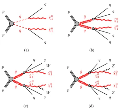
In this document SUSY signals are described by simplified models. They are defined by an e ff ective Lagrangian describing the interactions of a small number of new particles, assuming one production process and one decay channel with a 100% branching fraction. Signal samples are used to describe squark- and gluino-pair production, followed by the direct decays of squarks ( ˜ q → q χ ˜

) and direct ( ˜ g → q q ¯ χ ˜

) or one-step ( ˜ g → q qW ¯ χ ˜

, ˜ g → q qZ ¯ χ ˜

) decays of gluinos as shown in Figure 1. Direct decays are those where the considered SUSY particles decay directly into SM particles and the LSP, while the one-step decays refer to the cases where the decays occur via one intermediate on-shell SUSY particle, as indicated in parentheses. These samples are generated with up to two extra partons in the matrix element using MG5_aMC@NLO 2.2.2 event generator [36] interfaced to P ythia 8.186 [37]. The CKKW- L merging scheme [38] is applied with a scale parameter that is set to a quarter of the mass of the gluino for ˜ g g ˜ production or of the squark for ˜ q q ˜ production. The A14 [39] set of tuned parameters (tune) is used for underlying event together with the NNPDF2.3LO [40] parton distribution function (PDF) set.

The E vt G en v1.2.0 program [41] is used to describe the properties of the b- and c- hadron decays in the signal samples, and the background samples except those produced with S herpa [42]. The signal cross-sections are calculated at next-to-leading order (NLO) in the strong coupling constant, adding the resummation of soft gluon emission at next-to-leading-logarithmic accuracy (NLO + NLL) [43–47]. The nominal cross-section is taken from an envelope of cross-section predictions using di ff erent PDF sets and factorization and renormalization scales, as described in Ref. [48], considering only light-flavour quarks (u, d, s, c). For the light-flavour squarks (gluinos) in case of gluino- (squark-) pair production, cross-sections are evaluated assuming masses of 450 TeV. The free parameters are m

1

and m

(m

) for gluino-pair (squark-pair) production models.

The production of W or Z bosons in association with jets [49] is simulated using the S herpa 2.2.0 gener- ator, while the production of γ in association with jets is simulated using the Sherpa 2.1.1 generator. For W or Z bosons, the matrix elements are calculated for up to two partons at NLO and up to two additional partons at leading order (LO) using the C omix [50] and O pen L oops [51] matrix-element generators, and merged with the S herpa parton shower [52] using the ME + PS@NLO prescription [53]. The samples are produced with a simplified scale setting prescription in the multi-parton matrix elements, to improve the event generation speed. A theory-based re-weighting of the jet multiplicity distribution is applied at event level, derived from event generation with the strict scale prescription. Events containing a photon in association with jets are generated requiring a photon transverse momentum above 35 GeV. For these events, matrix elements are calculated at LO with up to three or four partons depending on the p

of the photon, and merged with the S herpa parton shower using the ME + PS@LO prescription [54]. In the case of W /Z +jets, the NNPDF3.0NNLO PDF set [55] is used, while for the γ +jets production the CT10 PDF set [56] is used, both in conjunction with dedicated parton shower-tuning developed by the authors of S herpa . The W/Z + jets events are normalized to their NNLO cross-sections [57]. For the γ + jets process the LO cross-section, taken directly from the Sherpa MC generator, is multiplied by a correction factor as described in Section 8.

For the generation of t¯ t and single-top processes in the Wt and s-channel [58], the Powheg-Box v2 [59]

generator is used with the CT10 PDF set. The electroweak (EW) t-channel single-top events are generated

(a) (b)

(c)

˜ g

˜ g

˜ χ⁰₂

˜ χ⁰₂ p

p

q q

˜ χ⁰₁ Z

q q

˜ χ⁰₁ Z

(d)

Figure 1: The decay topologies of (a) squark-pair production and (b, c, d) gluino-pair production, in the simplified models with (a) direct decays of squarks and (b) direct or (c, d) one-step decays of gluinos.

using the P owheg -B ox v1 generator. This generator uses the four-flavour scheme for the NLO matrix- element calculations together with the fixed four-flavour PDF set CT10f4 [56]. For this process, the decay of the top quark is simulated using MadSpin tool [60] preserving all spin correlations, while for all processes the parton shower, fragmentation, and the underlying event are generated using P ythia 6.428 [61] with the CTEQ6L1 [62] PDF set and the corresponding P erugia 2012 tune (P2012) [63]. The top quark mass is set to 172.5 GeV. The h

parameter, which controls the p

of the first additional emission beyond the Born configuration, is set to the mass of the top quark. The main e ff ect of this is to regulate the high-p

emission against which the ttbar system recoils [58]. The t¯ t events are normalized to the NNLO+NNLL [64, 65]. The s- and t-channel single-top events are normalized to the NLO cross-sections [66, 67], and the Wt-channel single-top events are normalized to the NNLO + NNLL [68, 69].

For the generation of t¯ t + EW processes (t¯ t + W/Z/WW ) [70], the MG5_aMC@NLO 2.2.3 [36] generator at LO interfaced to the P ythia 8.186 parton-shower model is used, with up to two (t¯ t + W, t¯ t + Z(→ νν/qq)), one (t¯ t + Z(→ ``)) or no (t¯ t + WW) extra partons included in the matrix element. The ATLAS underlying- event tune A14 is used together with the NNPDF2.3LO PDF set. The events are normalized to their respective NLO cross-sections [71, 72].

Diboson processes (WW , WZ, ZZ) [73] are simulated using the S herpa 2.1.1 generator. For processes

with four charged leptons (4`), three charged leptons and a neutrino (3` +1ν) or two charged leptons and

two neutrinos (2` +2ν), the matrix elements contain all diagrams with four electroweak vertices, and are

calculated for up to one (4`, 2` + 2ν) or no partons (3` + 1ν) at NLO and up to three partons at LO using the

Comix and OpenLoops matrix-element generators, and merged with the Sherpa parton shower using the

ME+PS@NLO prescription. For processes in which one of the bosons decays hadronically and the other

leptonically, matrix elements are calculated for up to one (ZZ) or no (WW , WZ) additional partons at NLO

and for up to three additional partons at LO using the Comix and OpenLoops matrix-element generators,

and merged with the S herpa parton shower using the ME + PS@NLO prescription. In all cases, the CT10 PDF set is used in conjunction with a dedicated parton-shower tuning developed by the authors of Sherpa.

The generator cross-sections are used in this case.

The multi-jet background is generated with Pythia 8.186 using the A14 underlying-event tune and the NNPDF2.3LO parton distribution functions.

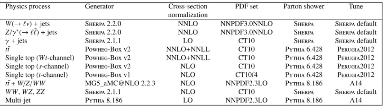
A summary of the SM background processes together with the MC generators, cross-section calculation orders in α

, PDFs, parton shower and tunes used is given in Table 1.

Physics process Generator Cross-section PDF set Parton shower Tune

normalization

W(→`ν)+jets Sherpa2.2.0 NNLO NNPDF3.0NNLO Sherpa Sherpadefault

Z/γ^∗(→``)¯ +jets Sherpa2.2.0 NNLO NNPDF3.0NNLO Sherpa Sherpadefault

γ+jets Sherpa2.1.1 LO CT10 Sherpa Sherpadefault

tt¯ Powheg-Boxv2 NNLO+NNLL CT10 Pythia6.428 Perugia2012

Single top (Wt-channel) Powheg-Boxv2 NNLO+NNLL CT10 Pythia6.428 Perugia2012 Single top (s-channel) Powheg-Boxv2 NLO CT10 Pythia6.428 Perugia2012 Single top (t-channel) Powheg-Boxv1 NLO CT10f4 Pythia6.428 Perugia2012

tt¯+W/Z/WW MG5_aMC@NLO 2.2.3 NLO NNPDF2.3LO Pythia8.186 A14

WW,WZ,ZZ Sherpa2.1.1 NLO CT10 Sherpa Sherpadefault

Multi-jet Pythia8.186 LO NNPDF2.3LO Pythia8.186 A14

Table 1: The Standard Model background Monte Carlo simulation samples used in this paper. The generators, the order inαsof cross-section calculations used for yield normalization, PDF sets, parton showers and tunes used for the underlying event are shown.

For all SM background samples the response of the detector to particles is modelled with a full ATLAS detector simulation [74] based on Geant4 [75]. Signal samples are prepared using a fast simulation based on a parameterization of the performance of the ATLAS electromagnetic and hadronic calorimeters [76]

and on G eant 4 elsewhere.

All simulated events are overlaid with multiple pp collisions simulated with the soft QCD processes of P ythia 8.186 using the A2 tune [39] and the MSTW2008LO parton distribution functions [77]. The simulations are reweighted to match the distribution of the mean number of interactions observed in data.

4. Object reconstruction and identification

The reconstructed primary vertex of the event is required to be consistent with the luminous region and to have at least two associated tracks with p

> 400 MeV. When more than one such vertex is found, the vertex with the largest P

p

of the associated tracks is chosen.

Jet candidates are reconstructed using the anti-k

jet clustering algorithm [78, 79] with jet radius parameter

of 0.4 and starting from clusters of calorimeter cells [80]. The jets are corrected for energy from pile-up

using the method described in Ref. [81]: a contribution equal to the product of the jet area and the median

energy density of the event is subtracted from the jet energy [82]. Further corrections, referred to as the

jet energy scale corrections, are derived from MC simulation and data and used to calibrate on average

the energies of jets to the scale of their constituent particles [83]. Only jet candidates with p

> 20 GeV

and |η| < 2.8 after all corrections are retained. An algorithm based on boosted decision trees, ‘MV2c10’

[84, 85], is used to identify jets containing a b-hadron (b-jets), with an operating point corresponding to an efficiency of 77%, along with the rejection factors of 134 for light-quark jets and 6 for charm jets [85].

Candidate b-tagged jets are required to have p

> 50 GeV and |η| < 2.5. Events with jets originating from detector noise and non-collision background are rejected if the jets fail to satisfy the ‘LooseBad’ quality criteria, or if at least one of the two leading jets with p

> 100 GeV fails to satisfy the ‘TightBad’ quality criteria, both described in Ref. [86]. These selections a ff ect less than 1% of the events used in the search.

In order to reduce the number of jets coming from pile-up, a significant fraction of the tracks associated with each jet must have an origin compatible with the primary vertex, as defined by the jet vertex tagger (JVT) output [87]. The requirement JVT > 0.59 is only applied to jets with p

< 60 GeV and |η| < 2.4.

Two different classes of reconstructed lepton candidates (electrons or muons) are used in the analyses presented here. When selecting samples used for the search, events containing a ‘baseline’ electron or muon are rejected. The selections applied to identify baseline leptons are designed to maximize the efficiency with which W +jets and top quark background events are rejected. When selecting ‘control region’ samples for the purpose of estimating residual W +jets and top quark backgrounds, additional requirements are applied to leptons to ensure greater purity of these backgrounds. These leptons are referred to as ‘high-purity’ leptons below and form a subset of the baseline leptons.

Baseline muon candidates are formed by combining information from the muon spectrometer and in- ner tracking detectors as described in Ref. [88] and are required to have p

> 10 GeV and |η| < 2.7.

High-purity muon candidates must additionally have |η| < 2.4, the significance of the transverse impact parameter with respect to the primary vertex, |d

|/σ(d

) < 3, the longitudinal impact parameter with respect to the primary vertex |z

sin(θ)| < 0.5 mm, and to satisfy ‘GradientLoose’ isolation requirements described in Ref. [88] which rely on the use of tracking-based and calorimeter-based variables and im- plement a set of η- and p

-dependent criteria. The leading, high-purity muon, is also required to have p

> 27 GeV.

Baseline electron candidates are reconstructed from an isolated electromagnetic calorimeter energy de- posit matched to an ID track and are required to have p

> 10 GeV, |η| < 2.47, and to satisfy ‘Loose’

likelihood-based identification criteria described in Ref. [89]. High-purity electron candidates addition- ally must satisfy ‘Tight’ selection criteria described in Ref. [89], and the leading electron must have p

> 27 GeV. They are also required to have |d

|/σ(d

) < 5, |z

sin(θ)| < 0.5 mm, and to satisfy similar isolation requirements as those applied to high-purity muons.

After the selections described above, ambiguities between candidate jets with |η| < 2.8 and leptons are resolved as follows: first, any such jet candidate which is not tagged as b-jet, lying within a distance

∆ R ≡ p

( ∆ y)

+ ( ∆ φ)

= 0.2 of a baseline electron is discarded. If a jet candidate is b-tagged, the object is interpreted as a jet and the overlapping electron is ignored. Additionally, if a baseline elec- tron (muon) and a jet passing the JVT selection described above are found within 0.2 ≤ ∆ R < 0.4 ( ∆ R <min(0.4, 0.04 + 10 GeV / p

)), the object is interpreted as a jet and the nearby electron (muon) candidate is discarded. Finally, if a baseline muon and jet are found within ∆ R < 0.2, the object is treated as a muon and the overlapping jet is ignored if the jet satisfies the following criteria: N

<

3 or

p

> 0.7 P

p

and p

< 0.5p

, where N

refers to the number of tracks with p

>

500 MeV that are to the jet, and P

p

is the sum of their transverse momenta. These criteria are in- tended to identify jets consistent with final state radiation or hard bremsstrahlung.

Additional ambiguities between electrons and muons in a jet, originating from the decays of hadrons,

are resolved to avoid double counting and/or remove non-isolated leptons: the electron is discarded if a

baseline electron and a baseline muon share the same ID track.

The measurement of the missing transverse momentum vector E

(and its magnitude E

) is based on the calibrated transverse momenta of all electron, muon, photon and jet candidates and all tracks originating from the primary vertex and not associated with such objects [90].

Reconstructed photons are not used in the main signal-event selection, but are used to select in the region to constrain the Z +jets background, as explained in Section 8. Photon candidates are required to satisfy p

> 150 GeV and |η| < 2.37, photon shower shape and electron rejection criteria [91], and to be isolated.

Ambiguities between candidate jets and photons (when used in the event selection) are resolved by dis- carding any jet candidates lying within ∆ R = 0.4 of a photon candidate. Additional selections to remove ambiguities between electrons or muons and photons are applied such that the photon is discarded if it is within ∆ R = 0.4 of an electron or muon.

Corrections derived from data control samples are applied to account for di ff erences between data and simulation for the lepton trigger and reconstruction e ffi ciencies, the lepton momentum / energy scale and resolution, and for the efficiency and mis-tag rate of the b-tagging algorithm.

5. The Recursive Jigsaw Reconstruction technique

The Recusive Jigsaw Reconstruction technique is a method used as a basis for defining the kinematic variables on an event-by-event level. While it is straightforward to fully describe an event’s underlying kinematic features when all objects are fully reconstructed, events involving weakly interacting particles present a challenge, as the loss of information constrains the kinematic variable construction to take place in the lab frame instead of the more physically natural frames of the hypothesized decays. The deconstruction of the available kinematic information into factorizable information is only possible given a set of external constraints on the invisible system (e.g. longitudinal boost invariance) and minimizations of the masses of intermediate particle states with respect to unknown quantities.

Given a rule for applying additional information to the invisible system, known here as a jigsaw, a specific

underlying decay hypothesis can be imposed on the event. The RJR algorithm is an inter-changeable rule

for resolving a kinematic or combinatoric ambiguities. By viewing the event in a certain decay topology

and accounting for the assumptions for the lost degrees of freedom, a four-momentum hypothesis is as-

signed to each invisible state. Once all four-momenta are defined, the RJR variable construction involves

boosting into proxy rest frames for each intermediate hypothesized particle. In these rest frames, kin-

ematic variables can be computed, and for the correct decay tree topology, variables from different rest

frames should encode different information and be therefore uncorrelated. A natural basis of observables

is then the one associated with this decay tree. The available variables can depend on the decay tree

topology used.

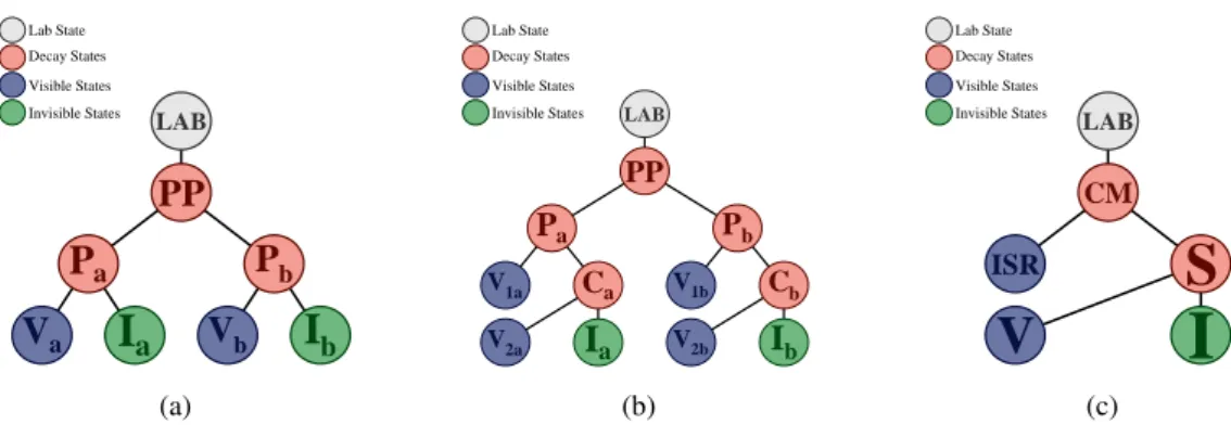
LAB

PP P

V

I

P

V

I

Lab State Decay States Visible States Invisible States

(a)

LAB

PP Pa V1a C_a

V2a

I

Pb V1b C_b V2b

I

Lab State Decay States Visible States Invisible States

(b)

LAB CM

ISR

S

V I

Lab State Decay States Visible States Invisible States

(c)

Figure 2: (a) Inclusive strong sparticle production decay tree. Two sparticles (PaandPb) are non-resonantly pair- produced with each decaying to one or more visible particles (VaandVb) which are reconstructed in the detector, and two systems of invisble particles (IaandIb) whose four-momenta are only partially constrained. (b) An additional level of decays can be added to the left tree when requiring more than two visible objects. This tree is particularly useful for the search for gluino pair-production described in the text. (c) Strong sparticle production with ISR decay tree for use with small mass-splitting spectra. A signal sparticle systemS decaying to a set of visible momentaV and invisible momentumIrecoils offof a jet radiation system ISR.

In searches for strong production of sparticles in R-parity conserving models, one can impose the decay tree shown in Figure 2(a). Each event is analyzed as if two sparticles (the intermediate states P

and P

) were produced and then decayed to the particles observed in our detector (the collections V

and V

).

The benchmark signal models probed in this search give rise to signal events with at least two weakly- interacting particles associated with two systems of particles (I

and I

), the respective children of the initially produced sparticles.

This decay tree includes several kinematic and combinatoric unknowns. In the final state with no leptons, the objects observed in the detector are exclusively jets and one must decide how to partition these jets into the two groups V

and V

in order to calculate the observables associated with the decay tree. In this case, the grouping that minimizes the masses of the four-vector sum of group constituents is chosen.

More explicitly, the collection of reconstructed jet four-vectors, V ≡ { p

} and their four-vector sum p

are considered. Each of the four-momenta is evaluated in the rest-frame of p

(V-frame) and di ff erent partitionings of these jets V

= { p

, · · · , p

} are considered such that V

T

V

= 0 and V

S

V

= V.

For each partition, the sum of four-vectors p

i

= P

j

p

is calculated and the combination chosen that maximizes the momenta of the two groups, |~ p

a

| + | ~ p

b

|. The axis that this partition implicitly defines in the V rest-frame is equivalent to the thrust-axis of the jets, and the masses M

= q

p

i

have, in a sense, been simultaneously minimized. When analyzing the entire event, these two groups are called “jet hemispheres.”

The remaining unknowns in the event are associated with the two collections of weakly interacting

particles: their masses, longitudinal momenta and information as how the two groups independently

contribute to the E

. The RJR algorithm organizes these unknowns into the groups of necessary in-

formation for determining the relative velocities of the reference frames in the decay tree, or the boosts

that relate them to each other. The algorithm then proceeds from the first known reference frame, the lab

frame, and traverses the decay tree through each intermediate frame. When unknowns are encountered

that are necessary to determine the following boosts, a jigsaw rule of choosing always the mass minimiz- ation of the hemispheres is applied to resolve the necessary information.

In each of these newly constructed rest frames, all relevant momenta are defined and can be used to construct any variable – multi-object invariant masses, angles between objects, etc. The primary scale- sensitive variables used in the search presented here are a suite of scale variables denoted by H. These H variables derive their name from H

, the scalar sum of visible transverse momenta. However, in contrast to H

, these H variables are constructed with aggregate momenta, including contributions from the invisible four-momenta, and are not necessarily evaluated in the lab frame, nor only in the transverse plane.

The H variables are labeled with a superscript F and two subscripts n and m, H

. The F represents the rest frame in which the momenta are evaluated. In this analysis, this may be the lab frame, the proxy frame for the sparticle-sparticle frame PP, or the proxy frame for an individual sparticle’s rest frame P. The subscripts n and m represent the number of visible and invisible momentum vectors considered, respectively. This means given the number of visible momentum vectors in the frame, these will be summed together until there remain only n distinct vectors. The choice for which vectors are summed is made by finding jets nearest in phase space. This is done using the same mass-minimization procedure used in the frame construction. This procedure tends to join, for example, a hard jet with a soft near-by radiated jet. The same is done for the invisible system into m vectors. For events with fewer than n visible objects the sum will only run over the available vectors. The additional subscript T can denote a transverse version of the variable where the transverse plane is defined with respect to the velocity of the frame F. In practice, this is similar to the plane transverse to the beam-line. The purposeful obfuscation of information into aggregate momenta allows for the same event to be interpreted in several independent ways such that each H variable encodes unique information.

In addition to scale-sensitive variables, the power of the RJR technique comes from the ensemble of variables that can be constructed and used in concert with the H variables with minimal correlation. It is therefore useful to categorize variables into those sensitive to scale (generally having units of GeV) and those that are unitless and scale-invariant. In the limit that one only places requirements on scale- invariant variables, there is no dependence on the sparticle spectrum and the sensitivity to compressed spectra is improved. In practice, this can guide the construction of regions targeting compressed spectra where stricter requirements on scale-invariant variables can be emphasized.

Given the plethora of choices the RJR technique provides, the variables that are used to define the signal and control regions, described in the document are listed below. The paradigm of the RJR analysis design is to use as few requirements with units GeV as possible. The sensitivity of the analysis is amplified by marrying a minimal set of scale variables requirements with selections imposed on unitless quantities.

To select signal events in models with squark-pair production, the following variables are used:

• H

→ scale variable as described above. Similar to E

.

• H

→ scale variable as described above. Similar to e ff ective mass, m

(defined as the scalar sum of the transverse momenta of the leading two jets and E

) for squark-pair production signals with two-jet final states.

• H

/H

→ provides additional information in testing the balance of the information provided by

the two scale cuts, where in the denominator the H

is no longer solely transverse. This provides

an excellent handle against imbalanced events where the large scale is dominated by a particular object p

or by high E

.

• p

/(p

+ H

) → compares the z-momentum of the lab frame to the overall transverse scale variable considered. This variable tests for significant boost in the z direction.

• p

/H

→ represents the fraction of the overall scale variable that is due to the second highest p

jet (in the PP frame) in the event.

For signal topologies with higher jet multiplicities, there is the option to exploit the internal structure of the hemispheres by using a decay tree with an additional decay. For gluino-pair production, the tree shown in Figure 2(b) can be used and the variables used by this search are:

• H

→ described above.

• H

→ analogous to the transverse scale variable described above but more appropriate for four- jet final states expected from gluino-pair production.

• H

/H

→ analogous to H

/H

for the squark search.

• H

/H

→ a measure of the fraction of the momentum that lies in the transverse plane.

• p

/(p

+ H

) → analogous to p

/( p

+ H

) above.

• min (p

/H

) → represents the fraction of a hemisphere’s overall scale due to the second highest p

jet (in the PP frame) in each hemisphere. The minimum value between the two hemi- spheres is used.

• max (H

/H

) → testing balance of solely the jets momentum in a given hemisphere allows an additional handle against a small but pernicious subset of events.

• |

∆ φ

−

cos θ

| → constructed from the difference between the azimuthal angle between the V and P frames, evaluated in the PP frame and the polar angle of that parent particle. The di ff erence between these two angular properties highlights events where the missing transverse momentum is imbalanced between hemispheres (e.g. semileptonic t¯ t decays where the lepton is reconstructed as a jet). This variable exploits the fact that signal events tend to be more “spherical” to e ffi ciently suppress these pernicious background sources.

In addition to trying to resolve the entirety of the signal event, it can be useful for sparticle spectra with smaller mass splittings and lower intrinsic E

to instead select for a partially-resolved sparticle system recoiling o ff of a high-p

jet from initial state radiation (ISR). To target such topologies, a separate tree targeting compressed spectra can be seen in Figure 2(c). This tree is somewhat simpler and attempts to identify visible (V ) and invisible (I ) systems that are the result of an intermediate state S . This signal system is required to recoil o ff of a system of visible momenta associated with the ISR. This tree yields a slightly di ff erent set of variables:

• |p

| → the magnitude of the vector-summed transverse momenta of all ISR-associated jets evalu-

ated in the CM frame.

• R

≡ ~ p

· p ˆ

/p

→ serves as a proxy for m

/m

. → This is the fraction of the boost of the S system that is carried by its invisible system I. As the |p

| is increased it becomes increasingly hard for backgrounds to possess a large value in this ratio - a feature exhibited by compressed signals.

• M

→ the transverse mass of the S system.

• N

→ number of jets assigned to the visible system (V ) and not associated with the ISR system.

• ∆ φ

→ This is the opening angle between the ISR system and the invisible system in the lab frame.

6. Analysis strategy and fit description

This section summarizes the common analysis strategy and statistical techniques that are employed in the searches presented in this document.

To search for a possible signal, selections are defined to enhance the signal relative to the SM background.

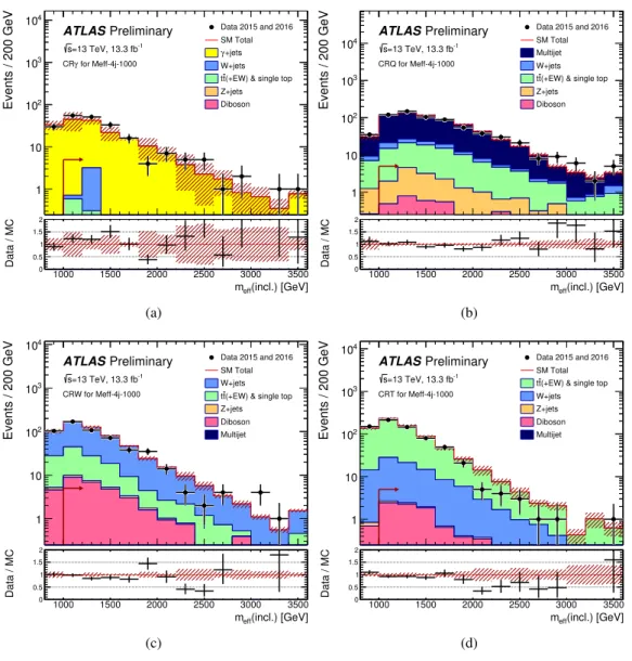
Signal regions (SRs) are defined using the Monte Carlo simulation of the signal processes and the SM backgrounds. They are optimized to maximize the expected significance for each model considered. To estimate the SM backgrounds in a consistent and robust fashion, corresponding control regions (CRs) are defined for each of the signal regions. They are chosen to be non-overlapping with the SR selections in order to provide independent data samples enriched in particular background sources, and are used to normalize the background MC simulation. The CR selections are optimized to have negligible SUSY signal contamination for the models near the previously excluded boundary [16], while minimizing the systematic uncertainties arising from the extrapolation of the CR event yields to estimate backgrounds in the SR. Cross-checks of the background estimates are performed with data in several validation regions (VRs) selected with requirements such that these regions do not overlap with the CR and SR selections, and also have a low expected signal contamination.

To extract the final results, three di ff erent classes of likelihood fit are employed: background-only, model- independent and model-dependent fits [92]. A background-only fit is used to estimate the background yields in each SR. The fit is performed using the observed event yields from the CRs associated with the SR as the only constraints, and not the SR itself. It is assumed that signal events from physics beyond the Standard Model (BSM) do not contribute to these yields. The scale factors (µ

, µ

, µ

, µ

) are fitted in each CR attached to a SR. The expected background in the SR is based on the yields predicted by simulation for W /Z + jets, top quark backgrounds, corrected by the scale factors derived from the fit. In case of multi-jet background, the estimate is based on the data-driven method described in Section 8. The systematic uncertainties and the MC statistical uncertainties in the expected values are included in the fit as nuisance parameters which are constrained by Gaussian distributions with widths corresponding to the sizes of the uncertainties considered and by Poisson distributions, respectively. The background-only fit is also used to estimate the background event yields in the VRs.

If no excess is observed, a model-independent fit is used to set upper limits on the number of BSM signal

events in each SR. This fit proceeds in the same way as the background-only fit, except that the number

of events observed in the SR is added as an input to the fit, and the BSM signal strength, constrained to

be non-negative, is added as a free parameter. The observed and expected upper limits at 95% confidence

level (CL) on the number of events from BSM phenomena for each signal region (S

and S

) are

derived using the CL

prescription [93], neglecting any possible signal contamination in the control re- gions. These limits, when normalized by the integrated luminosity of the data sample, may be interpreted as upper limits on the visible cross-section of BSM physics (hσi

), where the visible cross-section is defined as the product of production cross-section, acceptance and e ffi ciency. The model-independent fit is also used to compute the one-sided p-value (p

) of the background-only hypothesis, which quantifies the statistical significance of an excess.

Finally, model-dependent fits are used to set exclusion limits on the signal cross-sections for specific SUSY models. Such a fit proceeds in the same way as the model-independent fit, except that both the yield in the signal region and the signal contamination in the CRs are taken into account. Correlations between signal and background systematic uncertainties are taken into account where appropriate. Signal-yield systematic uncertainties due to detector effects and the theoretical uncertainties in the signal acceptance are included in the fit.

7. Event selection and signal regions definitions

Following the object reconstruction described in Section 4, in both searches documented here events are discarded if a baseline electron or muon with p

> 10 GeV remains, or if they contain a jet failing to satisfy quality selection criteria designed to suppress detector noise and non-collision backgrounds (described in Section 4). Only events with a reconstructed primary vertex associated with two or more tracks are used further in the analyses. Events are rejected if no jets with p

> 50 GeV are found. The remaining events are then analysed in two complementary searches, both of which require the presence of jets and significant missing transverse momentum. The selections in the two searches are designed to be generic enough to ensure sensitivity in a broad set of models with jets and E

in the final state.

In order to maximize the sensitivity in the (m

, m

) plane, a variety of signal regions are defined. They are chosen by optimizing the value of the signal discovery significance for a signal mass hypothesis defined to provide the value close to a 3 σ significance. Squarks typically generate at least one jet in their decays, for instance through ˜ q → q χ ˜

, while gluinos typically generate at least two jets, for instance through g ˜ → q q ¯ χ ˜

. Processes contributing to ˜ q q ˜ and ˜ g g ˜ final states therefore lead to events containing at least two or four jets, respectively. Decays of heavy SUSY and SM particles produced in longer ˜ q and ˜ g decay cascades (e.g. ˜ χ

→ qq

χ ˜

) tend to further increase the jet multiplicity in the final state. To target different scenarios, signal regions with di ff erent jet multiplicity requirements (in the case of Me ff -based search) or different decay trees (in the case of RJR-based search) are assumed. Summary of optimized signal regions used by both searches are presented in the following.

7.1. The jets + E

T

Me ff -based search

Due to the high mass scale expected for the SUSY models considered in this study, the ‘e ff ective mass’,

m

, is a powerful discriminant between the signal and SM backgrounds. When selecting events with

at least N

jets, m

(N

) is defined to be the scalar sum of the transverse momenta of the leading N

jets

and E

. Requirements placed on m

and E

form the basis of the Me ff -based search by strongly

suppressing the multi-jet background where jet energy mismeasurement generates missing transverse

momentum. The final signal selection uses requirements on both m

(incl.), which sums over all jets with

p

> 50 GeV and E

, which is required to be larger than 250 GeV.

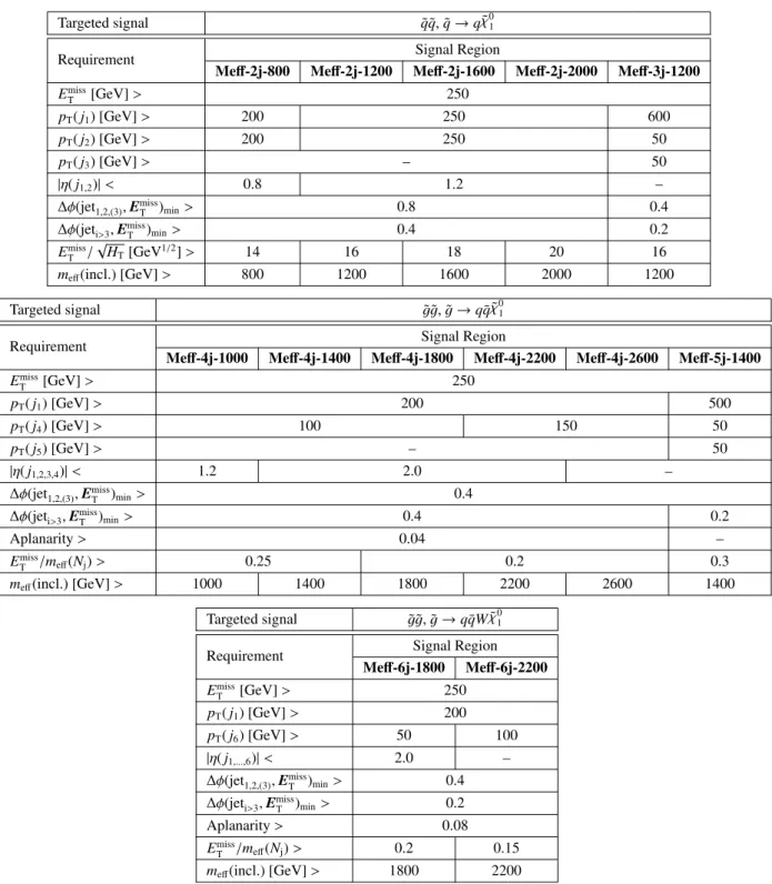
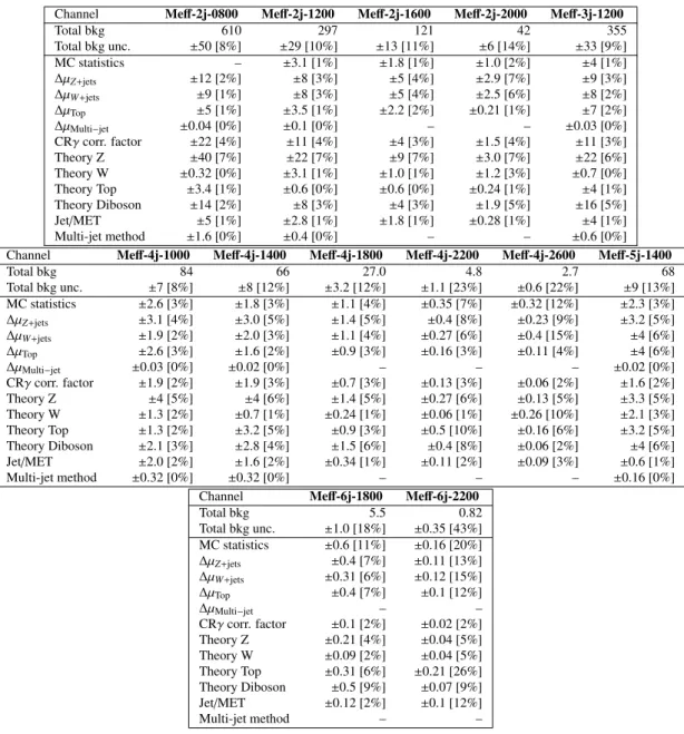
Thirteen inclusive SRs characterized by increasing minimum jet multiplicity from two to six, are defined in Table 2: five regions targeting models characterized by the squark-pair production with the direct decay of squarks, six regions targeting models with gluino-pair production followed by the direct decay of gluinos and two regions targeting gluino-pair production followed by the one-step decay of gluino via an intermediate chargino. Signal regions requiring the same jet-multiplicity are distinguished by increasing the threshold of the m

(incl.) and E

/m

(N

) (or E

/ √

H

) requirements. This ensures the sensitivity to di ff erent mass di ff erences for each decay mode. All signal regions corresponding to the Meff-based search have ‘Meff’ prefix.

In each region, di ff erent thresholds are applied on jet momenta and on ∆ φ(jet, E

)

, which is defined to be the smallest azimuthal separation between E

and the momenta of any of the reconstructed jets with p

> 50 GeV. Requirements on ∆ φ(jet, E

)

and E

/m

(N

) are designed to reduce the background from multi-jet processes. For the 2-jet SRs which are optimized for squark-pair production followed by the direct decay of squarks, the selection requires ∆ φ(jet

, E

)

> 0.8 using up to three leading (if jets present in the event), while in SRs with higher jet multiplicities the requirement

∆ φ(jet

, E

)

> 0.4 is used. For the SRs requiring at least four, five or six jets in the final state, or in the case when more than three jets are present in 2-jet or 3-jet SRs, an additional requirement on

∆ φ(jet

, E

)

is applied to all jets.

In the 2-jet and 3-jet SRs the requirement on E

/m

(N

) is replaced by a requirement on E

/ √

H

(where H

is defined as the scalar sum of the transverse momenta of all jets), which is found to lead to

enhanced sensitivity to models characterized by ˜ q q ˜ production. In the other regions with at least four

jets in the final state, additional suppression of background processes is based on the aplanarity variable,

which is defined as A = 3/2λ

, where λ

is the smallest eigenvalue of the normalized momentum tensor

of the jets [94].

Targeted signal q˜˜q, ˜q→qχ˜⁰₁

Requirement Signal Region

Meff-2j-800 Meff-2j-1200 Meff-2j-1600 Meff-2j-2000 Meff-3j-1200

E_T^miss[GeV]> 250

pT(j1) [GeV]> 200 250 600

pT(j2) [GeV]> 200 250 50

pT(j3) [GeV]> – 50

|η(j1,2)|< 0.8 1.2 –

∆φ(jet1,2,(3),E^miss_T )min> 0.8 0.4

∆φ(jeti>3,E^miss_T )min> 0.4 0.2 E_T^miss/√

HT[GeV^1/2]> 14 16 18 20 16

meff(incl.) [GeV]> 800 1200 1600 2000 1200

Targeted signal g˜˜g, ˜g→q¯qχ˜⁰₁

Requirement Signal Region

Meff-4j-1000 Meff-4j-1400 Meff-4j-1800 Meff-4j-2200 Meff-4j-2600 Meff-5j-1400

E^miss_T [GeV]> 250

pT(j1) [GeV]> 200 500

pT(j4) [GeV]> 100 150 50

pT(j5) [GeV]> – 50

|η(j1,2,3,4)|< 1.2 2.0 –

∆φ(jet1,2,(3),E^miss_T )_min> 0.4

∆φ(jeti>3,E^miss_T )min> 0.4 0.2

Aplanarity> 0.04 –

E^miss_T /meff(Nj)> 0.25 0.2 0.3

m_eff(incl.) [GeV]> 1000 1400 1800 2200 2600 1400

Targeted signal g˜˜g, ˜g→qqW¯ χ˜⁰₁

Requirement Signal Region

Meff-6j-1800 Meff-6j-2200

E^miss_T [GeV]> 250

pT(j1) [GeV]> 200

pT(j6) [GeV]> 50 100

|η(j1,...,6)|< 2.0 –

∆φ(jet1,2,(3),E^miss_T )min> 0.4

∆φ(jeti>3,E^miss_T )min> 0.2

Aplanarity> 0.08

E^miss_T /m_eff(Nj)> 0.2 0.15 meff(incl.) [GeV]> 1800 2200

Table 2: Selection criteria and targeted signal model used to define signal regions in the Meff-based search, in- dicated by the prefix ‘Meff’. Each SR is labelled with the inclusive jet multiplicity considered (‘2j’, ‘3j’ etc.) together with the degree of background rejection. The latter is denoted by the value corresponding to the meff

cut. The E^miss_T /m_eff(Nj) cut in anyNj-jet channel uses a value ofmeff constructed from only the leadingNj jets (m_eff(N_j)). However, the finalmeff(incl.) selection, which is used to define the signal regions, includes all jets with pT >50 GeV.

7.2. The jets + E

T

RJR-based search

As with the Me ff -based search, various signal regions are defined in the RJR-based approach to be most sensitive to a variety of proposed signal hypotheses. It is chosen to limit the number of “scale variables"

(those with units GeV) to only two when defining the signal regions targeting models with gluino- and squark-pair production. The various collections of signals are grouped according to sparticle mass split- tings with dedicated optimizations. The two chosen scale variables are H

and either H

(for models targeting squark-pair production) or H

(for models targeting gluino-pair production). These serve to leverage events with large missing momentum and a high collective scale of visible objects in events. In order to further suppress SM backgrounds, a variety of additional constraints on unitless variables are imposed.

In general, the procedure follows that as the mass splitting between parent sparticle and LSP increases, the criteria applied to the scale variables are tightened, while the criteria on unitless variables are loosened. In searching for the squark-pair production, the overall balance of the events is studied with H

/H

. The range selected in this ratio aims to reject those events where the missing transverse momentum dominates the scale (upper requirement) and to ensure sufficient balance between the scales (lower requirement).

The selection on the p

/H

ratio serves to ensure that each of the jets contributes to the overall scale significantly. This particular ratio is a powerful criterion against imbalanced V +jets events, where one of the jets has a much higher momentum than the sub-leading jet. In order to protect against events where the z-component of the laboratory frame momentum dominates the scale, we select this ratio to be low.

For gluino-pair produced signals, the same principles are followed. Tight requirements are placed on H

/H

and H

/H

to target scenarios with compressed spectra. As with the squark case a ratio selection is used, on p

/

p

+ H

in this case, to test the size of the z-component relative to the overall scale. A lower threshold is placed on the ratio of the second jet divided by the scale of the hemisphere. This provides a very strong constraint against events where the two hemispheres are well- balanced but one of the jets dominates the scale variable contribution. As described in Section 5, the

|

∆ φ

−

cos θ

| variable serves to e ffi ciently protect against high jet multiplicity events, mostly arising from top-quark processes, where the E

would be mostly associated with a single hemisphere.

Additionally, separate SRs are defined for models with compressed spectra. Following the pattern of successive SRs targeting larger mass-splitting scenarios, several regions designed to be sensitive to vari- ous mass-splittings utilize the ISR-boosted compressed decay tree described in Section 5. These regions target mass-splittings from roughly 25 GeV to 200 GeV, in increasing order.

These variables in concert serve to provide criteria to reject each of the major backgrounds while e ffi - ciently maintaining signal candidates for the processes considered. In order to reject events where the E

results from mis-measurements of jets, the E

is associated with one or more jets using a trans- verse clustering scheme, identifying those jets which are closest in phase-space. The variable ∆

considers the magnitude of E

, the transverse momentum of the associated jets, along with the azi- muthal angle between the two, in order to quantify the likelihood that mis-measurements of these jets were responsible for the E

. Multi-jet events with severe jet mis-measurements tend to have ∆

values between [-1,0] while events with E

from weakly-interacting particles prefer [0,1]. The variable is defined as the signed asymmetry between

• the transverse momentum of the associated jet system that projects onto the direction of the E

system normalized to this value summed with the E

and