s = 8 TeV with the ATLAS detector

(1)

ATLAS-CONF-2013-092 28August2013

ATLAS NOTE

ATLAS-CONF-2013-092

August 27, 2013

Search for long-lived, heavy particles in final states with a muon and a multi-track displaced vertex in proton-proton collisions at √

s = 8 TeV with the ATLAS detector

The ATLAS Collaboration

Abstract

Many extensions of the Standard Model posit the existence of new heavy particles with long lifetimes. Results are presented of a search for such particles, which decay at a sig- nificant distance from their production point, using a final state containing charged hadrons and an associated muon. This analysis uses a data sample of proton-proton collisions at

√s =

8 TeV corresponding to an integrated luminosity of 20.3 fb

⁻¹

collected in 2012 by

the ATLAS detector operating at the Large Hadron Collider. Results are interpreted in the context of

R-parity violating supersymmetric scenarios.

No events in the signal region are observed, with an expected background of 0.02

±

0.02 events, and 95% confidence level limits are set on squark pair production processes where the squark decays into the lightest supersymmetric particle (the neutralino) followed by the decay of the neutralino into a muon and quarks, and for neutralino lifetime

τ

between 3 ps and 3 ns (cτ between 1 mm and 1 m). To allow these limits to be used in a variety of models, they are presented for a range of squark and neutralino masses.

c

Reproduction of this article or parts of it is allowed as specified in the CC-BY-3.0 license.

(2)

1 Introduction

Several extensions to the Standard Model predict the production at the Large Hadron Collider (LHC) of heavy particles with lifetimes that can be in the picosecond-to-nanosecond range [1]. The decays of such particles form a unique signature of vertices that are displaced from the proton-proton interaction point (IP). One such scenario is supersymmetry with

R-parity violation (RPV) [2, 3]. The present (largely

indirect) constraints on RPV couplings [2, 3] would allow the decay of the lightest supersymmetric particle as it traverses a particle detector at the LHC. Signatures of heavy, long-lived particles also feature in models of gauge-mediated supersymmetry breaking [4], split-supersymmetry [5], hidden-valley [6], dark-sector gauge bosons [7] and stealth supersymmetry [8].

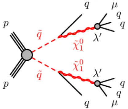
This note presents the results of a search for the decay of a heavy particle, producing a multi-track vertex that contains a high transverse momentum (

p_T

) muon, at a distance between millimeters and tens of centimeters from the

pp

interaction point. As in the previous searches carried out by ATLAS [9, 10], the results are interpreted in the context of an

R-parity-violating supersymmetric scenario. In this model,

the signature corresponds to the decay of the lightest supersymmetric particle, resulting in a muon and many charged tracks originating from a single displaced vertex (DV). This decay can arise from a diagram such as that shown in Fig. 1, where the decay is mediated by the non-zero RPV coupling

λ⁰_{2i j}

. It should however be noted that this search will also be sensitive to other models, including those with long-lived charged particles, that decay with the same displaced vertex signature.

Searches for related signatures have also been made at the Tevatron with

√

s =

1.96 TeV

pp

¯ col- lisions. The DØ collaboration has searched for a long-lived neutral particle decaying into a final state containing two muons [11] or a

bb

¯ pair [12]. Similar searches have also been made at LEP [13]. The CMS collaboration has searched for long-lived particles decaying into two jets [14].

The search reported here uses a dataset with an integrated luminosity of 20.3 fb

⁻¹

[15], which is more than four times greater than that of the previous ATLAS search for this signature [9]. The

pp

collision energy has been increased to

√

s=

8 TeV, resulting in higher cross-sections for the production of heavy particles. The analysis procedure and event selection are mostly unchanged with respect to Ref. [9], where additional information on these techniques can be found. Some modifications to the trigger and event selection criteria are implemented to address the higher number of

pp

collisions per bunch crossing (pile-up) in the 2012 data. The method for background estimation is modified to be independent of the possible presence of hadronically decaying long-lived particles.

This note is organised as follows. The ATLAS detector, and the data samples used in this study are introduced in Sections 2 and 3. Section 4 then describes the selection and reconstruction of muons and displaced vertices (DVs). Determination of the signal e

ffi

ciency, including the calculation of its variation with

cτ

is detailed in Section 5. The background estimation is covered in Section 6, and in particular, Section 6.1 describes what turns out to be the dominant (though still very small) source of background:

vertices arising from hadronic interactions with gas molecules, which coincide with other tracks in the same event. Systematic uncertainties are listed in Section 7, and finally, results are presented in Section 8.

2 The ATLAS detector

The ATLAS detector [16] is a multipurpose apparatus at the LHC. The detector consists of several layers of subdetectors. From the IP outwards, these are an inner detector (ID) for measuring the tracks of charged particles, electromagnetic and hadronic calorimeters, and an outer muon spectrometer (MS).

The ID is immersed in a 2 Tesla axial magnetic field, and extends from a radius

¹

of about 45 mm to

1ATLAS uses a right-handed coordinate system with its origin at the nominal IP in the centre of the detector and thez-axis along the beam pipe. Thex-axis points from the IP to the centre of the LHC ring, and they-axis points upward. Cylindrical coordinates (R, φ) are used in the transverse plane,φbeing the azimuthal angle around the beam pipe. The pseudorapidity is

(3)

Figure 1: Feynman diagram of the signal model considered in this note, with squark pair production, and the long-lived lightest neutralino ˜

χ⁰₁

decaying into a muon and two quark jets via the lepton-number and

R-parity violating couplingλ⁰_{2i j}

.

1100 mm and to

|z|

of about 2750 mm. It provides tracking and vertex information for charged particles within the pseudorapidity region

|η|<

2.5. At small radii, silicon pixel layers and stereo pairs of silicon microstrip sensors provide high resolution pattern recognition. The pixel system consists of three barrel layers, and three forward disks on either side of the interaction point. The barrel pixel layers, which are positioned at radii of 50.5 mm, 88.5 mm, and 122.5 mm are of particular relevance to this work. The silicon microstrip tracker (SCT) comprises four double layers in the barrel, and nine forward disks on either side. A further tracking system, a transition-radiation tracker (TRT), is positioned at larger radii.

This device is made of straw-tube elements interleaved with transition-radiation material and provides coverage within

|η|<

2.0. Muon identification and momentum measurement is provided by the MS. This device has a coverage in pseudorapidity of

|η| <

2.7 and is a 3-layer system of gas-filled precision-tracking chambers. The pseudorapidity region

|η|<

2.4 is additionally covered by separate trigger chambers, used by the level-1 hardware trigger. The MS is immersed in a magnetic field which is produced by a barrel toroid and two end-cap toroids.

Online event selection is made with a three-level trigger system. This system comprises a hardware- based level-1 trigger, which uses information from the MS trigger chambers and the calorimeters, fol- lowed by two software-based trigger levels.

3 Data and simulation

The data used in this analysis were collected between April and December 2012. After the application of beam, detector, and data-quality requirements, the total luminosity of the data is 20.3 fb

⁻¹

. The uncertainty on the integrated luminosity is

±2.8%. It is derived, following the same methodology as

that detailed in Ref. [15], from a preliminary calibration of the luminosity scale derived from beam- separation scans performed in November 2012. It is required that the trigger identifies a muon candidate with transverse momentum

p_T >

50 GeV and

|η| <

1.05. The

|η|

selection is imposed due to the larger fake-muon rate in the (higher

|η|) end-cap region. This trigger algorithm identifies muons using the MS

only, not requiring a matching ID track.

Signal events are generated with P



6 [17], using the MRST LO** [18] set of parton distribu- tion functions (PDFs). The simulated processes include production of a ˜

qq, ˜

˜

q^∗q

˜

^∗

, or ˜

qq

˜

^∗

pair in the

pp

collision, with each squark (antisquark) decaying into a long-lived lightest neutralino and a quark (anti- quark). Degeneracy of the first and second generations and of the left-handed and right-handed squarks

defined in terms of the polar angleθasη=−ln tan(θ/2).

(4)

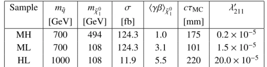
Sample

mq_˜ m_χ_˜0

1 σ hγβi_χ_˜0

1 cτ_MC λ⁰₂₁₁

[GeV] [GeV] [fb] [mm]

MH 700 494 124.3 1.0 175 0.2

×

10

⁻⁵

ML 700 108 124.3 3.1 101 1.5

×

10

⁻⁵

HL 1000 108 11.9 5.5 220 20.0

×

10

⁻⁵

Table 1: The parameter values for the three signal MC samples used in this work: the assumed squark mass, production cross-section (calculated at NLO

+

NLL as described in the text), neutralino mass, av- erage value of the Lorentz boost factor (from P [17]), average proper lifetime multiplied by

c, and

value of

λ⁰₂₁₁

coupling used in the generation of the signal MC samples.

is assumed. The masses of the gluino, sleptons and third generation squarks are set to a high value and are thus not directly produced in the supersymmetry scenario that is simulated.

The parameter settings for the samples of signal Monte Carlo (MC) files are summarised in Table 1.

The chosen values of squark and neutralino masses span a wide range in the quantities to which the signal e

ffi

ciency is most sensitive, namely, the neutralino speed and the final-state multiplicities (see Section 5).

The signal MC samples are labeled in Table 1 according to the squark mass and neutralino mass, respec- tively: MH (medium-mass squark, heavy neutralino), ML (medium-mass squark, light neutralino), and HL (heavy squark, light neutralino). It is assumed that all RPV couplings other than

λ⁰₂₁₁

are zero, so that neutralino decays to

µ⁻ud

¯ (or the charge-conjugate state)

²

. The values of the

λ⁰₂₁₁

coupling in the various samples are selected such that a significant fraction of neutralino decays occur in the detector volume considered in this analysis. Values for

c

multiplied by the average neutralino-proper-lifetimes used in the generation of the samples, (cτ

_MC

) are provided in Table 1. The

p_T

distributions for muons in the MH and HL samples are shown in Fig. 2.

Figure 2: The transverse-momentum distributions of signal muons in the (left) MH sample and the (right) HL sample (which is similar to the distribution for the ML sample).

Signal cross-sections are calculated to next-to-leading order in the strong coupling constant, adding the resummation of soft gluon emission at next-to-leading-logarithmic accuracy (NLO+NLL) [19, 20, 21, 22, 23]. The nominal cross-section and the uncertainty are taken from an envelope of cross-section pre- dictions using different PDF sets and factorisation and renormalisation scales, as described in Ref. [24].

Cross-section values are listed in Table 1.

2In the SUSY scenario assumed here, a non-zeroλ⁰₂₁₁can also lead to the decay of a neutralino to a neutrino and jets final state with the same branching fraction as for the muonic decay. For this reason, exclusion limits for a 50% branching ratio for the neutralino to decay to a charged muon plus jets, will be presented alongside those for a 100% branching ratio.

(5)

Samples of dijet background were generated with P



8 [25] and are used for comparison of track variables between data and MC and for obtaining the systematic uncertainty related to the tracking efficiency. Finally, a sample of

Z → µ⁺µ⁻

events generated using S [26] was used to estimate systematic uncertainties associated with the trigger.

Each generated event in the signal or background samples is processed with the Geant4-based [27]

ATLAS detector simulation [28] and treated in the same way as the collision data. The generated samples include a realistic modelling of the pile-up conditions observed in the data.

4 Vertex reconstruction and event selection

Events in our muon-triggered sample are required to contain at least one reconstructed displaced vertex (DV) identified using the Inner Detector, and a high-p

_T

reconstructed muon. Details of the event, muon, and vertex selection requirements are listed in the following sub-sections.

4.1 Event and muon selection

Due to the high instantaneous luminosity of the LHC in 2012, most events contain more than one primary vertex (PV). The PV with the highest sum of the

p²_T

values of the tracks associated to it is required to have at least five tracks and a

z

position (z

_PV

) in the range

|z_PV| <

200 mm. We use the symbol PV to refer only to this vertex, unless explicitly indicating that it refers to all the PVs in the event.

Events must contain a muon candidate that is reconstructed in both the MS and the ID with transverse momentum

p_T >

55 GeV (which is chosen so as to be at the beginning of the e

ffi

ciency plateau of the trigger),

|η| <

1.07 (also based on the acceptance of the trigger), and a transverse impact parameter that satisfies

|d₀| >

1.5 mm, where

d₀

is the impact parameter of the track with respect to the transverse position of the PV, which is labeled (x

_PV, y_PV

). To ensure that the muon candidate is associated with the muon that satisfied the trigger requirement, the selection

p

∆φ²+ ∆η²<

0.15 is imposed, where

∆φ

(∆

η)

is the difference between the azimuthal angle (pseudorapidity) of the reconstructed muon candidate and that of the muon identified by the trigger. The ID track associated with the muon candidate is required to have at least five SCT hits, with at most one SCT hit that is expected to be in an active and functioning detector element, but is not found. Furthermore, the track must satisfy an

η-dependent requirement on

the number of TRT hits. No pixel-hit requirements are applied to the muon track, in order to accept tracks with large

d₀

. The requirements described above are referred to as the muon-selection criteria.

If an event contains two reconstructed muons, they are required to satisfy

p

(π

−∆φ)²+

(η

₁+η₂

)

²>

0.1, where

∆φ

is the di

ff

erence in azimuthal angles of the two muons, and

η₁

and

η₂

are their pseudo- rapidities. This requirement strongly suppresses cosmic-ray background, where a single muon is recon- structed as two back-to-back muons.

4.2 Track reconstruction and selection

To ensure the high quality of tracks used in the reconstruction of a displaced vertex, the candidate tracks must have two or more associated SCT hits, and transverse momentum greater than 1 GeV. In order to reject tracks originating from primary

pp

interactions, we require the tracks to satisfy

|d₀| >

2 mm.

Standard ATLAS track reconstuction [16] is based on three passes in which the initial track “seed”

candidates are formed in one of three ways: tracks may be initially found in the silicon detectors, initially found in the TRT, or found only in the TRT. These algorithms all assume that tracks originate from close to the PV, and hence have reduced reconstruction e

ffi

ciency for signal tracks, which originate at a DV.

We counter this limitation and recover signal tracks via a procedure termed “re-tracking”, in which the

silicon-seeded tracking algorithm is re-run on ID hits that are not used for tracks from standard tracking,

(6)

with the loose requirements

|d₀⁰| <

300 mm and

|z⁰₀| <

1500 mm, where

d₀⁰

and

z⁰₀

are the transverse and

z-direction impact parameters with respect to the origin of the coordinate system. Plots showing the

efficiency improvement brought about by re-tracking can be found in Ref. [9].

4.3 Displaced vertex reconstruction

DVs are reconstructed from the selected tracks using an algorithm based on the incompatibility-graph approach [29]. The DV reconstruction method is similar to that used in Ref. [30]. The algorithm begins by finding two-track seed vertices from all pairs of tracks. Pairs that have a vertex-fit

χ²

of less than 5 are retained. A seed vertex is rejected if either of its tracks has hits between the vertex and the PV.

Multi-track vertices are formed, based on these seed vertices, in an iterative process, as follows. If a track is assigned to two di

ff

erent vertices, the action taken depends on the distance

D

between the vertices. If

D <

3σ

D

, where

σD

is the estimated uncertainty on

D, a single vertex is formed from the tracks of

the two vertices. Otherwise, the track is associated with the vertex for which the track-to-vertex fit has the smaller

χ²

value. If this value exceeds six, the track is removed from the vertex, and the vertex is refitted. This process continues until no track is associated with more than one vertex. Finally, vertices are combined and refitted if they are separated by less than 1 mm. This value was optimized in MC studies, and found to give rise to a slight increase in e

ffi

ciency via combining sets of tracks from the same true neutralino decay that had been reconstructed as separate DVs, with no appreciable increase in background.

For DVs with three-or-more tracks and radial position inside the third pixel layer, the typical DV position resolution in the signal MC samples is tens of microns for

r_DV

and about 200

µm forz_DV

. For vertices beyond the outermost pixel layer, which is located at a radius of 122.5 mm, the typical resolution is several hundred microns for both coordinates. For two-track vertices, the typical resolution is about

200

µm forr_DV<

122.5 mm, and several millimetres for larger radii.

4.4 Displaced vertex selection

To ensure a good quality DV fit, the

χ²

per degree of freedom of the fit must be less than 5. Furthermore, the DV position is required to be in the fiducial region, defined as:

|z_DV|<

300 mm and

r_DV <

180 mm, where

r_DV

and

z_DV

are the radial and longitudinal vertex positions with respect to the origin, respectively.

To minimise background due to tracks originating from the hard scatter or pileup primary vertices, the transverse distance

p

(x

_DV−x_PV

)

²+

(y

_DV−y_PV

)

²

between the DV and any of the PVs must be at least 4 mm, which also removes most vertices arising from heavy-flavour decays.

In order to mitigate the effects of fake tracks, which are more prevalent in the high pile-up conditions in 2012 than in previous years, vertices containing one or more badly-reconstructed tracks are removed.

These tracks are defined as those where the relative uncertainty on any of the five measured track parame- ters (azimuthal angle, polar angle, transverse and longitudinal impact parameter, and inverse momentum) is greater than 10%.

Displaced vertices from particle-material interactions are abundant in regions in which the detector

material is dense. To reduce this source of background, vertices that are reconstructed in regions of

high-density material are removed. This criterion is referred to as the material veto. The high-density

material is mapped using material-interaction candidate vertices in data and true material-interaction

vertices in minimum-bias MC events. The

z_DV

and

r_DV

positions of these vertices are used to make

a two-dimensional material-density distribution with a bin size of 4 mm in

z_DV

and 1 mm in

r_DV

. It

has been demonstrated [30] that the detector simulation describes well the positions of pixel layers and

associated material, while the simulated position of the beampipe is shifted with respect to the actual

position. The use of data events to construct the material map therefore ensures that the beampipe

material is correctly mapped, while the use of the simulation provides a high granularity of the map at

(7)

the outer pixel layers, where material-interaction vertices in the data are comparatively rare. Material- map bins with vertex density greater than an

r_DV

- and

z_DV

-dependent density criterion are characterised as high-density-material regions. These regions correspond to 34% of the volume within

|z_DV|<

300 mm,

r_DV<

180 mm, and are visible in Fig. 3.

A signal region is defined in terms of the number of tracks,

N_t

, in the DV, and

m_DV

, the invariant mass of the set of tracks associated with the DV, using the charged pion mass hypothesis for each track.

This signal region, which was selected based on control sample distributions before looking at the data, is chosen to be

N_t ≥

5 and

m_DV >

10 GeV, which reduces background from random combinations of tracks and from material interactions. Candidate vertices that pass (fail) the

m_DV>

10 GeV requirement are hereafter referred to as being high-m

DV

(low-m

DV

) vertices.

Finally, to ensure that the muon candidate is associated with the reconstructed DV, the DOCA (dis- tance of closest approach) of the muon with respect to the DV is required to be less than 0.5 mm. If the reconstructed muon trajectory passes within about 0.01 mm of the DV position, the muon track is usually included as one of the tracks in the vertex. Studies on MC have shown that the DOCA ¿ 0.5 mm requirement increases the e

ffi

ciency by 50% relative to requiring the muon to be one of the tracks in the vertex, with a negligible increase in the probability of associating the wrong muon to the vertex.

The muon-to-vertex association is imposed only at the end of the selection chain, in order that some sensitivity be retained for scenarios where the muon and DV do not come from the same source, by noting whether any candidate events survive the selections up to this point.

The aforementioned selections are collectively referred to as the vertex-selection criteria.

5 Signal e ffi ciency

The signal e

ffi

ciency depends strongly on the e

ffi

ciencies for track reconstruction and track selection, which are a

ff

ected by the following factors:

1. Heavier neutralinos will give rise to larger number of tracks originating from the DV, and a larger total invariant mass from these tracks. The reconstruction e

ffi

ciency is correspondingly higher.

2. More tracks fail the

|d₀|>

2 mm requirement for small

r_DV

or if the neutralino is highly boosted, so that the trajectories of its daughters point back to close to the PV.

3. The track reconstruction e

ffi

ciency decreases slowly with

|d₀|, and hence withr_DV

.

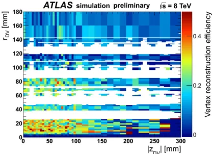
Figure 3 shows the vertex-reconstruction e

ffi

ciency for the MH sample as a function of (|z

_DV|,r_DV

) after all selection criteria, including the material veto.

The single-vertex selection efficiency for each of the signal MC samples is shown in Fig. 4 as a func- tion of

cτ. Although the signal MC samples are each generated using a single cτ

value (see Table 1), the kinematics of these samples can be used to generate simulated distributions of neutralino decay posi- tions for many different

cτ

values. Each of these distributions is then combined with a two-dimensional e

ffi

ciency map in (|z

DV|,r_DV

) (shown in Fig. 3 for the “MH” sample) to obtain the vertex reconstruction e

ffi

ciency at that

cτ

value. Figure 4 includes systematic corrections and uncertainties that are discussed in Section 7.

The final event-selection e

ffi

ciency for each of the signal MC samples, which takes into account the

fact that each signal event contains two signal neutralino decays, is also shown in Fig. 4. This e

ffi

ciency

accounts also for the muon selection requirements and their systematic uncertainties.

(8)

Figure 3: The e

ffi

ciency as a function of

r_DV

and

z_DV

for vertices in the MH signal-MC sample. The blank areas represent regions of dense material that are not considered when looking for DVs. It is evident that some areas of this map su

ff

er from limited MC statistics, leading to large bin-to-bin fluctuations. This is accounted for by recalculating this map many times, varying each bin content within its statistical uncertainty.

Figure 4: The left plot shows the efficiency for single vertex reconstruction as a function of

cτ

for the

three signal MC samples. The right plot shows the efficiency for reconstructing at least one DV in the

event under the assumption that there are two signal neutralinos in the event. The dashed lines represent

the envelopes corresponding to statistical and systematic uncertainties on the efficiency.

(9)

6 Background estimation

Spurious high-m

_DV

, high-multiplicity vertices in non-material regions may originate from one of two sources:

1. Vertices from real hadronic interactions with gas molecules outside the beampipe. Although most of these events have masses below the 10 GeV requirement, the high mass tail of the distribution indicates a potential background, in particular if the vertex is crossed by a non-associated track (real or fake) at a large crossing angle.

2. Purely random combinations of tracks (real or fake). This type of background is expected to form the largest contribution at small radii, where the track density is highest, and is the only background in the vacuum region inside the beampipe.

The yield of both types of background is estimated considering first the background vertexing e

ffi

ciency, assuming it can be factorized from the trigger and muon-related efficiency, which are considered later.

6.1 Background outside the beampipe

The background from real hadronic interactions, including those crossed by tracks originating from dif- ferent PVs, are obtained separately in four regions corresponding to (1) the volume between the beampipe and the innermost pixel layer, (2-3) the two regions between adjacent pixel layers, and (4) outside of the outermost pixel layer. Two distributions of

m_DV

are constructed from a large control sample of 12 million jet-triggered events, and are used to model the

m_DV

distribution of background vertices with

N_t

tracks.

The first distribution,

P^N_nc^t

(m

DV

), called the “non-crossing” distribution, is formed from

N_t

-track vertices that do not contain a track that forms a large angle with respect to all other tracks in the vertex. The selection requirement for these vertices is that for each track in the vertex, the average angle with respect to all other tracks in the vertex is less than 0.5 radian. The second, “crossing” distribution

P_c^N^t

(m

DV

) is formed by adding the four-momentum of each (N

t−

1)-track vertex to that of a randomly-selected track in the same event. Taking

P^N_nc^t

(m

_DV

) and

P^N_c^t

(m

_DV

) to be normalized so that their integrals in the range 0

< m_DV < ∞

equal unity, the total yield and

m_DV

distribution of the background for

N_t ≥

3 vertices is modeled as a linear combination of these functions.

N_tot^N^tP^N^t

(m

DV

)

= N_tot^N^t

(

f_ncP^N_nc^t

(m

DV

)

+ f_cP^N_c^t

(m

DV

))

≡N_nc^N^tP^N_nc^t

(m

DV

)

+N_c^N^tP^N_c^t

(m

DV

). (1) Two methods are used to obtain the scale factors that will be used to multiply the

P^N^t

functions in order to obtain an estimate of the number of vertices passing the (N

t

,

m_DV

) signal criteria in each region. These procedures, denoted the “3-track vertex template method” and the “K

S

method”, are described in the following sections.

6.1.1 The 3-track vertex template method

In this method, the coe

ffi

cients

f_nc^N^t

and

f_c^N^t

in Eq. 1 are determined so as to match the shape of the

m_DV

distribution of 3-track vertices, as illustrated in Fig. 5. The same values of

f_nc

and

f_c

are then used for

N_t>

3 vertices. The overall scale factor

N_tot^N^t

is found such that the integral of

N_tot^N^tP^N^t

(m

DV

) from zero to

2.5 GeV matches the corresponding integral of the

m_DV

distribution for

N_t

-track vertices. The integral of

the scaled function

N_tot^N^tP^N^t

(m

_DV

) from 10 GeV to infinity provides an estimate of the expected number

of background vertices.

(10)

6.1.2 TheKS method

In the

K_S

method, we scale the “crossed”

m_DV

distribution

P_c^N^t

by a factor

N_c^N^t

, given by

N_c^N^t = N^N^t⁻¹R_c,

(2)

where

N^N^t⁻¹

is the number of vertices with

N_t−

1 tracks. The “crossing ratio”

R_c

is the estimated ratio between the number of (N

_t−

1)-track vertices that are crossed by a random track to form an

N_t

-track vertex and the number of (N

t−

1)-track vertices that are not crossed. The ratio

R_c

is obtained by dividing the number of

K_S

mesons in 3-track vertices, which is found by fitting the invariant-mass distribution of all 2-track combinations within 3-track vertices, by the number of

KS

mesons forming 2-track vertices, found by fitting the invariant-mass distribution of 2-track vertices. No requirement is made on the total charge when forming 2-track combinations. The crossing ratio ranges from (2

±

1)

×

10

⁻⁴

in region 1 to (69

±

4)

×

10

⁻⁴

in region 4, where the uncertainties are statistical only.

The coefficient

N_nc^N^t

for the “non-crossed” distribution is obtained by ensuring that the integral of the total function

N_tot^N^tP^N^t

(m

DV

) from 0–2.5 GeVmatches the number of

N_t

-track vertices in that mass range. As with the 3-track-template method, the integral of the distribution

N_tot^N^tP^N^t

(m

DV

) from 10 GeV to infinity then gives an estimate for the number of

N_t

-track background vertices.

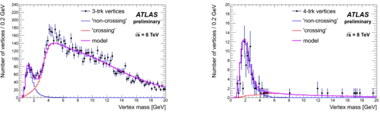
Figure 5: The

m_DV

distribution of 3-track (left) and 4-track (right) vertices in the jet-triggered control sample, in region 4 (the region outside the third pixel layer), with the model of Eq. (1) overlaid (magenta histogram). The peak at low

m_DV

is accounted for mostly by the “non-crossing” first term of Eq. (1), shown by the blue histogram, and the high-m

DV

region is fit well by the “crossing” second term (red histogram). The coe

ffi

cients in Eq. (1) for the left plot were obtained using the “3-trk” method, while the

“K

S

method” was used for the right plot.

6.1.3 Summary of background outside the beampipe

It should be noted that both methods are expected to over-estimate the background, since both use infor- mation about how many 3-track vertices are actually 2-track vertices crossed by a non-associated track, to estimate this proportion for higher

N_t

. However, since the position resolution for 2-track vertices is considerably worse than that for vertices with more tracks, the “crossing fraction” for 2-track vertices is correspondingly higher, giving rise to a larger normalisation factor for the

P^N_c^t

distribution than would be obtained if it were possible to accurately determine the crossing fractions for (N

_t >

2)-track vertices.

Of the two methods, the

KS

method might be expected to be more accurate, since it uses more infor-

mation (i.e. the number of (N

t−

1)-track vertices as well as the number of

N_t

-track vertices) to make

its predictions. However, the discrepancy between the data and the model at around 4 GeV for the 3-

track vertices in Fig. 5, shows that while the model seems to be qualitatively correct, the precise

m_DV

shape is not perfect. It is therefore desirable to use both of the two complementary methods to obtain

(11)

the normalisations of the “crossing” and “non-crossing” distributions, in order to provide an estimate of how variations in the di

ff

erent components of the

m_DV

distribution can give rise to di

ff

erences in the final background estimate.

Background estimates from the two methods are shown in Table 2 for each of the four regions, and are checked by comparing them with the numbers observed for

N_t =

3, 4. It is seen that the 3-track-vertex method is more reliable in predicting the number of 3-track vertices, while the

KS

method predicts the 4-track vertices better as expected. The 3-track-vertex method predicts higher background yields for

N_t ≥

3. The average of the predictions for the two methods in each region is used, with half of the difference as a systematic uncertainty on the background estimate.

Assuming that the number of

N_t >

6 background vertices is negligible, the total background estimate for

N_t ≥

5 background vertices in the control sample is obtained by summing the mean of the estimates for the “K

S

” and “3-trk template” methods for 5-track and 6-track vertices in each region from Table 2.

This gives an estimate of 17

±

16, where the uncertainty is both statistical and systematic. Scaling this estimate by the ratio of the number of events in the muon-triggered search sample to the number of events in the jet-triggered control sample yields a final background estimate of 0.02

±

0.02 vertices for the search sample.

6.2 Background inside the beampipe

Inside the beampipe, background due to material interactions is negligible due to the high vacuum.

However, the high particle density at small

r_DV

may result in high random-combination background. To estimate this background, we take advantage of the fact that the last step in the vertexing algorithm is the merging of vertices that are within 1 mm of each other. Therefore, a 4-track vertex may be formed by two 2-track vertices that happen to be less than 1 mm apart, or a 3-track vertex accidentally crossed by an unrelated track. Corresponding scenarios exist for higher-N

t

vertices.

To estimate the probability for two vertices to be within 1 mm with a high-statistics sample, we plot the distance between two vertices in di

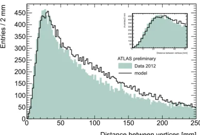
ff

erent events from another large control sample of 14 million events, collected using a mixture of different triggers. Figure 6 compares this distribution for 2-track vertices in different events and in the same event, validating the use of vertices from different events for this purpose. Although there is some disagreement at large separation distances, the region close to 1 mm, which is relevant for this background estimation method, compares well between the two distributions.

To estimate the probability for a vertex with

N_t−

1 tracks to be crossed by a track and form an

N_t

-track vertex, we use the crossing ratio

R_c

estimated with the

K_S

method inside the beampipe.

Table 3 shows the predicted number of background vertices of each type in this mixed-trigger control sample.

Adding the predictions of 5- and 6-track vertices and scaling them to the number of events in the search sample relative to that in the control sample yields an estimate of 4

×

10

⁻⁵

vertices inside the beampipe. A 300% relative uncertainty is assigned to this estimate, which covers the difference between the estimated and observed numbers of 4-track vertices.

6.3 Total background estimate

The study described in Section 6.2 demonstrates that the contribution to the background arising from

random combinations of tracks in the volume inside the beampipe is negligible. Therefore, the total

background prediction is dominated by the background outside the beampipe, which is estimated to be

0.02

±

0.02 vertices.

(12)

Re gion

Nt=

3

Nt=

4

Nt=

5

Nt=

6

KS

3-trk Obs

KS

3-trk Obs

KS

3-trk

KS

3-trk 1 24

±

6 46

±

4 43 0

.

10

±

0

.

01 3

.

6

±

0

.

8 0 (1

.

8

±

0

.

3)

×

10

−3

0

.

9

±

0

.

4 (0

±

3)

×

10

−3

0

.

3

±

0

.

2 2 350

±

90 190

±

10 162 0

.

6

±

0

.

2 24

±

4 0 0

.

07

±

0

.

02 5

.

7

±

0

.

9 (0

±

6)

×

10

−3

4

.

1

±

0

.

8 3 460

±

120 230

±

10 217 1

.

3

±

0

.

3 29

±

5 1 0

.

15

±

0

.

04 7

.

3

±

1

.

0 0

.

04

±

0

.

01 1

.

8

±

0

.

5 4 4200

±

1000 4300

±

200 3639 13

±

3 52

±

12 12 0

.

10

±

0

.

03 11

±

4 0

.

03

±

0

.

01 1

.

9

±

1

.

1 T able 2: The number of background v ertices in the jet-triggered control sample predicted by the

KS

method (

KS

) and the 3-track-v erte x method (3-trk) to satisfy all b ut the muon selection criteria for

Nt=

3

,

4

,

5

,

6. The errors sho wn are statistical only . F or

Nt=

3

,

4 the number of observ ed v ertices (Obs) is also sho wn.

(13)

Distance between vertices [mm]

0 50 100 150 200 250

Entries / 2 mm

0 50 100 150 200 250 300 350 400 450

ATLAS preliminary Data 2012 model

Distance between vertices [mm]

0 10 20 30 40 50

# entries/2 mm

0 50 100 150 200 250 300 350 400 450

Figure 6: The distribution of distances between pairs of 2-track vertices in the same event (shaded histogram) and in di

ff

erent events (unshaded histogram), in the mixed-trigger control sample described in Section 6.2. The two distributions are normalized to the same area in the region from 0–50 mm. The inset plot zooms in on this 0–50 mm range.

N_t=

4

N_t =

5

N_t =

6

2

+

2 3

+

1 Obs 3

+

2 4

+

1 4

+

2 3

+

3 5

+

1

0.3

±

0.3 1.5

±

0.4 5 (2

±

2)

×

10

⁻³

0.07

±

0.02 (4

±

4)

×

10

⁻⁵

0 (6

±

2)

×

10

⁻³

Table 3: Predicted numbers of mixed-trigger-control-sample background vertices inside the beampipe

from random combinations of vertices and tracks, using the “distance” method for (n

+m)-track combi-

nations and the crossing ratio

R_c

for (n

+

1)-track vertices crossed by one track. For

N_t =

4, the number

of observed vertices (Obs) is also given.

(14)

7 E ffi ciency corrections and systematic uncertainties

Several categories of uncertainties and e

ffi

ciency corrections are considered, using the methods devel- oped for our previous work [9].

Uncertainty on the signal reconstruction efficiency results from the limited size of the signal MC datasets as well as uncertainties in the e

ffi

ciencies of the trigger, tracking, and muon reconstruction.

Uncertainties due to the simulation of event pile-up and on the integrated luminosity are also included.

To estimate the uncertainty on the efficiency as a function of

cτ

(Fig. 4) from finite MC statistics, the e

ffi

ciency in each bin of the 2D e

ffi

ciency maps (Fig. 3) is varied randomly within its statistical uncer- tainty and the total e

ffi

ciency is repeatedly re-measured. The spread in those results is the contribution to the systematic uncertainty on the efficiency at each

cτ

value.

To compensate for the di

ff

erent

z-distributions of the primary vertices in data and MC simulation, a

weight is applied to each simulated event such that the reweighted

z_PV

distribution matches that in data.

This weight is applied to both the numerator and denominator in the efficiency calculation.

Similarly, a weight is applied to each simulated event such that the distribution of

µ, the average

number of interactions per bunch-crossing, matches that in data. An uncertainty associated with this procedure is estimated by varying the scaling applied to the

µ

values used as input to this correction calculation by

±10% and evaluating the diff

erences on the e

ffi

ciency as a function of

cτ. This diff

erence is applied as a symmetric systematic uncertainty.

A trigger efficiency correction and associated systematic uncertainty are derived from a study of

Z →µ⁺µ⁻

events in which at least one of the muons is selected with a single-muon trigger. The ratio of the trigger e

ffi

ciency in data and simulation is applied as a correction factor, and the statistical uncertainty from this method is added in quadrature to the differences between the

Z→µ⁺µ⁻

sample and the signal MC samples to obtain a systematic uncertainty.

The systematic uncertainty on the track reconstruction e

ffi

ciency is estimated by comparing the track finding performance between data and MC simulation. The uncertainty is estimated from a study where the number of

KS

vertices in data and simulation are compared over a range of radii and

η-values. Based

on the largest discrepancy seen in the double-ratio of

K_S

yields at large radii to the yield at small radius, in data and MC, 5% of tracks in the signal MC are randomly removed from the input to the vertexing algorithm, and the same procedure to obtain efficiency-vs-cτ is performed. The difference between this and the nominal e

ffi

ciency at each

cτ

point is taken as a systematic uncertainty.

Since the distribution of the true values of

d₀

for cosmic-ray muons is flat over the limited

d₀

range considered here, as confirmed by cosmic-ray simulation, a comparison of the shapes of the measured

d₀

- spectrum of cosmic muons, and the muon reconstruction e

ffi

ciency as a function of

d₀

on simulated signal MC samples, can be used to determine the accuracy to which the simulation reproduces the muon-finding efficiency. The ratio of these two

d₀

distributions is calculated, normalised by the totals in the range 2

<|d₀|<

4 mm. For a perfect simulation with negligible statistical uncertainties this distribution should be flat. However, variations are observed which can be attributed to an imperfect detector simulation or to statistical uncertainties related to the finite size of the simulated samples. All deviations from unity for the various samples are taken into account in the calculation of the signal e

ffi

ciency in each

d₀

bin. The statistical uncertainties from this procedure are propagated to uncertainties of between

±

6% and

±

10%

on the signal vertex reconstruction efficiency, depending on the signal sample. In the case that there are two muons per event, this uncertainty is treated as 100% correlated between them.

The magnitudes of the various contributions to the uncertainty on the signal e

ffi

ciency are listed in

Table 4, and are reflected in Figs. 3 and 4.

(15)

MH ML HL

MC statistics (1–7)% (4–12)% (7–20)%

Muon efficiency (6–8)% (5–7)% (5–7)%

Tracking efficiency (2.5–4.5)% (3.5–4.5)% (4–5.5)%

Trigger e

ffi

ciency 1.8% 1.8% 1.8%

Pile- up (0.5–2)% (0.5–2)% (1.5–2.5)%

Table 4: Summary of relative systematic uncertainties on the efficiency for values of

cτ

between 0.8 mm and 1 m.

8 Results

Figure 7 shows the distribution of

m_DV

vs.

N_t

for vertices in events passing trigger and event-selection requirements, but no o

ffl

ine muon requirements, and for vertices passing all requirements apart from those on

m_DV

and

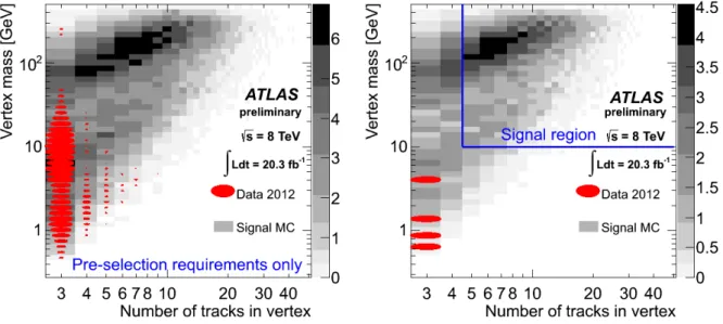
N_t

. The corresponding signal distributions for the MH sample are also shown. The signal region, corresponding to a minimum number of tracks in a vertex of five and a minimum vertex mass of 10 GeV, which was defined before looking at the data, is marked. No vertices are observed in the signal region.

Figure 7: The left plot shows vertex mass (m

DV

) vs. vertex track multiplicity (N

t

) for reconstructed DVs in non-material regions, in events that pass the trigger and primary vertex requirements. The right plot shows the same distribution for DVs where all event, muon, and vertex selection requirements are satisfied. Only four vertices in the data meet these criteria. Shaded bins show the distribution for the signal MC MH sample (see Table 1), and data are shown as filled ellipses, with the area of the ellipse proportional to the number of vertices in the corresponding bin.

Based on the observation of zero candidates in data, a 95% confidence-level (CL) upper limit of 0.14 fb is set on the visible cross-section, that is the production cross-section

σ

for any new physics process multiplied by the detector acceptance and the reconstruction e

ffi

ciency for that process.

Although an event is only required to contain one reconstructed DV (with associated muon) to be

considered “signal”, for models featuring pair-production such as the

R-parity-violating SUSY scenario

(16)

considered here, there could be one or two true candidates per event, depending on the branching ratio (BR) for the whole decay chain from squark to neutralino to muon-plus-quarks. The e

ffi

ciency for an event to pass all selection criteria (

_evt

) is related to the BR and the efficiency for a single vertex (

DV

) (shown in Fig. 4) via:

_evt=

2

×

BR

×_DV−

BR

²×_DV² .

(3)

Upper limits at 95% CL on the squark production cross-section

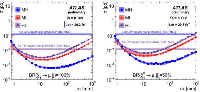
σ, corresponding to BR=

100% and BR=50%, are shown in Figure 8. These are obtained using the

CLs

method [31], using the profile likelihood as a test statistic, and with the uncertainties on efficiency, background, and luminosity treated as nuisance parameters. The NLO

+

NLL predictions for the production cross-sections for 700 GeV and 1000 GeV squark pairs are shown as bands, which represent the variation in predicted cross-section when using two different sets of PDFs (CTEQ6.6 and MSTW [32, 33]) and varying the factorisation and renormalisation scales each up and down by a factor of two. Since essentially no background is expected and no events are observed, the expected and observed limits are indistinguishable.

In addition, since the association between the reconstructed DV and muon is only made at the very last stage of the selection, an upper limit can be obtained for the situation where both a muon and a DV are reconstructed in the event, but not necessarily associated to one another. The corresponding 95%

upper limits are 0.8 fb for the “MH” sample, 2.9 fb for the “ML” sample, and 5.4 fb for “HL”. Note that these cross-section limits are only applicable at the values of

cτ_MC

listed in Table 1, since the

cτ

dependence of the e

ffi

ciency for reconstructing a muon that did not come from the same true neutralino decay as the DV is non-trivial.

Figure 8: Upper limits at 95% CL on

σ

vs. the neutralino lifetime for di

ff

erent combinations of squark

and neutralino masses, based on the observation of zero events satisfying all criteria in a 20.3 fb

⁻¹

data sample, for the case where the branching ratio for the decay chain from squark to neutralino to

muon-plus-jets is 100% (left), or 50% (right). The shaded areas around these curves represent the

±1σ

uncertainty bands on the expected limits. The horizontal lines show the cross-sections at NLO+NLL

for squark masses of 700 GeV and 1000 GeV, and the shaded regions around these lines represent the

uncertainties on the cross-sections obtained from the procedure described in the text.

(17)

9 Conclusions

Using a data sample of 20.3 fb

⁻¹

recorded by the ATLAS detector at the Large Hadron Collider in 2012,

an updated search is performed for new, heavy particles that decay at radial distances between 4 mm and

180 mm from the

pp

interaction point, in association with a high-transverse-momentum muon. For a

background estimate of 0.02

±

0.02 background events, no events are observed. Limits are presented on

the di-squark production cross-section in a SUSY scenario where the lightest neutralino produced in the

primary-squark decay undergoes an

R-parity-violating decay into a muon and two quarks. The limits are

reported as a function of the neutralino lifetime and for a range of neutralino masses and velocities, which

are the factors with greatest impact on the limit. Branching ratios of 50% and 100% for the decay chain

from squarks to neutralinos to muon-plus-quarks are considered. Limits for a variety of other models can

thus be estimated from these results, based on the neutralino mass, velocity, and multiplicity distribution

in a given model.

(18)

References

[1] M. Fairbairn, A. C. Kraan, D. A. Milstead, T. Sj¨ostrand, P. Z. Skands and T. Sloan, “Stable massive particles at colliders”, Phys. Rept.

438

(2007) 1, arXiv:hep-ph/0611040.

[2] R. Barbier, C. Berat, M. Besancon, M. Chemtob, A. Deandrea, E. Dudas, P. Fayet and S. Lavignac

et al., “R-parity violating supersymmetry”, Phys. Rept.420

(2005) 1, arXiv:hep-ph/0406039.

[3] B. C. Allanach, M. A. Bernhardt, H. K. Dreiner, C. H. Kom and P. Richardson, “Mass Spectrum in R-Parity Violating mSUGRA and Benchmark Points”, Phys. Rev. D

75

(2007) 035002,

arXiv:hep-ph/0609263.

[4] S. Dimopoulos, M. Dine, S. Raby and S. D. Thomas, “Experimental signatures of low-energy gauge mediated supersymmetry breaking”, Phys. Rev. Lett.

76

(1996) 3494,

arXiv:hep-ph/9601367.

[5] J. L. Hewett, B. Lillie, M. Masip and T. G. Rizzo, “Signatures of long-lived gluinos in split supersymmetry”, JHEP

0409

(2004) 070, arXiv:hep-ph/0408248.

[6] M. J. Strassler and K. M. Zurek, “Echoes of a hidden valley at hadron colliders”, Phys. Lett. B

651

(2007) 374, arXiv:hep-ph/0604261.

[7] P. Schuster, N. Toro and I. Yavin, “Terrestrial and Solar Limits on Long-Lived Particles in a Dark Sector”, Phys. Rev. D

81

(2010) 016002, arXiv:0910.1602 [hep-ph].

[8] J. Fan, M. Reece, J. T. Ruderman, “Stealth Supersymmetry”, JHEP

1111

(2011) 012, arXiv:1105.5135 [hep-ph].

[9] ATLAS Collaboration, “Search for long-lived, heavy particles in final states with a muon and multi-track displaced vertex in proton-proton collisions at

√

s=

7 TeV with the ATLAS detector,”

Phys. Lett. B

719, (2013) 280,

arXiv:1210.7451 [hep-ex].

[10] ATLAS Collaboration, “Search for displaced vertices arising from decays of new heavy particles in 7 TeV pp collisions at ATLAS”, Phys. Lett. B

707

(2012) 478, arXiv:1109.2242 [hep-ex].

[11] V. M. Abazov

et al.

[D0 Collaboration], “Search for neutral, long-lived particles decaying into two muons in

pp

¯ collisions at

√

s=

1.96 TeV”, Phys. Rev. Lett.

97

(2006) 161802, arXiv:hep-ex/0607028.

[12] V. M. Abazov

et al.

[D0 Collaboration], “Search for Resonant Pair Production of long-lived particles decaying to

bb

¯ in

pp

¯ collisions at

√

s=

1.96 TeV”, Phys. Rev. Lett.

103

(2009) 071801, arXiv:0906.1787 [hep-ex].

[13] G. Abbiendi

et al.

[OPAL Collaboration], “Searches for Gauge-Mediated Supersymmetry Breaking Topologies in

e⁺e⁻

collisions at LEP2”, Eur. Phys. J. C

46

(2006) 307-341, arXiv:hep-ex/0507048.

[14] CMS Collaboration, “Search for long-lived neutral particles decaying to dijets”, CMS-PAS-EXO-12-038 (2013).

[15] ATLAS Collaboration, “Improved Luminosity Determination in

pp

Collisions at

√

s=

7 TeV

using the ATLAS Detector at the LHC”, arXiv:1302.4393 [hep-ex].

(19)

[16] ATLAS Collaboration, “The ATLAS Experiment at the CERN Large Hadron Collider”, JINST

3

(2008) S08003.

[17] T. Sj¨ostrand, S. Mrenna and P. Z. Skands, “PYTHIA 6.4 Physics and Manual,” JHEP

0605

(2006) 026, arXiv:hep-ph/0603175.

Version used is 6.426.

[18] A. Sherstnev and R. S. Thorne, “Parton distributions for the LHC”, Eur. Phys. J

C55

(2009).

[19] W. Beenakker, R. Hopker, M Spira, P.M. Zerwas, “Squark and gluino production at hadron colliders”, Nucl. Phys.B492 (1997) 51-103, arXiv:hep-ph/9610490.

[20] A. Kulesza, L. Motyka, “Threshold resummation for squark-antisquark and gluino-pair production at the LHC”, Phys. Rev. Lett.

102

(2009) 111802, arXiv:0807.2405 [hep-ph].

[21] A. Kulesza, L. Motyka, “Soft gluon resummation for the production of gluino-gluino and squark-antisquark pairs at the LHC”. Phys. Rev.

D80

(2009) 095004, arXiv:0905.4749 [hep-ph].

[22] W. Beenakker

et al., “Soft-gluon resummation for squark and gluino hadroproduction”, JHEP 0912

(2009) 041, arXiv:0909.4418 [hep-ph].

[23] W. Beenakker

et al., “Squark and gluino hadroproduction”, Int. J. Mod. PhysA26

(2011) 2637-2664, arXiv:1105.1110 [hep-ph].

[24] M. Kramer

et al., “Supersymmetry production cross-sections in pp collisions at sqrt(s)=

7 TeV”, arXiv:1206.2892 [hep-ph].

[25] T. Sj¨ostrand, S. Mrenna and P. Skands, A. Comput. Phys. Comm.

178

(2008) 852, Version used is Pythia 8.160.

[26] T. Gleisberg

et al., “Event generation with SHERPA 1.1”, JHEP0902

(2009) 007, arXiv:0811.4622 [hep-ph].

Version used is Sherpa 1.4.1.

[27] S. Agostinelli

et al.

[GEANT4 Collaboration], “GEANT4: A Simulation toolkit”, Nucl. Instrum.

Meth. A

506

(2003) 250.

[28] ATLAS Collaboration, “The ATLAS Simulation Infrastructure”, Eur. Phys. J. C

70

(2010) 823, arXiv:1005.4568 [physics.ins-det].

[29] S. R. Das, “On a new approach for finding all the modified cut-sets in an incompatibility graph”, IEEE Transactions on Computers v22(2) (1973) 187.

[30] ATLAS Collaboration, “A study of the material in the ATLAS inner detector using secondary hadronic interactions”, JINST

7

(2012) 01013, arXiv:1110.6191 [hep-ex].

[31] A. L. Read, “Presentation of search results: The CL

s

technique”, J. Phys. G: Nucl. Part. Phys.28 (2002) 2693.

[32] P. M. Nadolsky, H. -L. Lai, Q. -H. Cao, J. Huston, J. Pumplin, D. Stump, W. -K. Tung and C. -P. Yuan, “Implications of CTEQ global analysis for collider observables”, Phys. Rev. D

78

(2008) 013004, arXiv:0802.0007 [hep-ph].

[33] A. D. Martin, W. J. Stirling, R. S. Thorne and G. Watt, “Parton distributions for the LHC”, Eur.

Phys. J. C

63

(2009) 189, arXiv:0901.0002 [hep-ph].

(20)

10 Appendix

ML MH HL

Event and muon selection cuts

All evts (100.

±

0.0)% (100.

±

0.0)% (100.

±

0.0)%

Good data quality (100.

±

0.0)% (100.

±

0.0)% (100.

±

0.0)%

Passes trigger (54.5

±

0.20)% (63.6

±

0.19)% (52.6

±

0.23)%

Primary vertex requirements (48.8

±

0.20)% (56.9

±

0.20)% (52.5

±

0.23)%

Event contains muon (48.8

±

0.20)% (56.9

±

0.20)% (52.4

±

0.23)%

Passes cosmics veto (48.7

±

0.20)% (56.7

±

0.20)% (52.3

±

0.23)%

Muon

p_T

,

η,d₀

requirements (43.2

±

0.20)% (54.4

±

0.20)% (46.4

±

0.23)%

Muon matched to trigger (41.6

±

0.20)% (52.6

±

0.20)% (44.3

±

0.23)%

Muon has good ID track (27.0

±

0.18)% (46.1

±

0.20)% (24.2

±

0.19)%

Vertex selection cuts

Event contains DV (27.0

±

0.18)% (46.0

±

0.20)% (24.1

±

0.19)%

DV in fiducial volume (25.6

±

0.17)% (45.4

±

0.20)% (21.8

±

0.19)%

DV

>

4 mm from PV in (x, y) (25.5

±

0.17)% (45.3

±

0.20)% (21.7

±

0.19)%

DV fit

χ²/

DoF< 5 (25.4

±

0.17)% (45.2

±

0.20)% (21.5

±

0.19)%

Track quality cuts (22.3

±

0.16)% (42.8

±

0.20)% (17.8

±

0.17)%

Passes material veto (15.5

±

0.14)% (34.9

±

0.19)% (11.7

±

0.14)%

DV

N_t≥

5 (5.70

±

0.09)% (19.3

±

0.16)% (3.13

±

0.08)%

m_DV>

10 GeV (5.09

±

0.08)% (18.5

±

0.15)% (2.72

±

0.07)%

DV matched to muon (3.33

±

0.07)% (13.1

±

0.13)% (1.65

±

0.05)%

Table 5: Event selection e

ffi

ciency for each signal sample following the sequential application of each

selection criterion. The initial number of events in each sample is 60 000. Muon-efficiency weights,

which can be larger than unity (see Section 7), are applied from the muon

p_T