ATLAS-CONF-2018-011 04/07/2018
ATLAS CONF Note
ATLAS-CONF-2018-011
13 May 2018
Measurement of the azimuthal anisotropy of charged particle production in Xe+Xe collisions at
√ s NN =5.44 TeV with the ATLAS detector
The ATLAS Collaboration
This note describes the measurement of flow harmonics
v2–
v5in Xe+Xe collisions at
√sNN
=5.44 TeV performed using the ATLAS detector at the LHC. The measurements are performed using multi-particle correlations involving 2, 4 and 6 particles and the Scalar Product technique. Measurements of the centrality and
pTdependence of the
vnare presen- ted. Comparisons of the measured
vnto previous measurements for Pb+Pb collisions at
√sNN
=5.02 TeV are also presented. The Xe+Xe
vnare observed to be larger than the Pb+Pb
vnfor
n=2,3 and 4 in the most central events, but with decreasing centrality or increasing harmonic order
n, the Xe+Xe
vnbecome smaller than the Pb+Pb
vn. The Xe+Xe and Pb+Pb comparisons are also shown as a function of the mean number of participants
hNparti, and the 4-particle cumulants for higher-order harmonics –
v3{4
}and
v4{4
}– are found to scale better with
hNpartithan with centrality. Comparisons of the
vnmeasurements to theoretical calculations are also made.
© 2018 CERN for the benefit of the ATLAS Collaboration.
Reproduction of this article or parts of it is allowed as specified in the CC-BY-4.0 license.
1 Introduction
Heavy ion collisions such as those at the Large Hadron Collider (LHC) [1] produce a new state of matter commonly termed quark-gluon plasma (QGP). The QGP produced in such collisions expands anisotropically, driven by spatial anisotropies in the initial geometry, which produce asymmetric pressure gradients between the medium and the outside vacuum. As it expands it cools and finally hadronizes.
Detailed investigations, based on hydrodynamics, have shown that the produced medium has properties similar to a nearly perfect fluid characterised by a very low ratio of viscosity to entropy density,
η/s[2].
The single-particle azimuthal yields of particle produced in heavy ion collisions are typically characterised as a Fourier series [2] :
dN dφ = N0
2
π1
+2
Σ∞n=1vncos
(n(φ−Φn)),(1) where
φis the azimuthal angle of the particle momentum, and the harmonics
vnand phases
Φnare the magnitude and phase of the
nth-order anisotropy. The
vnare typically functions of
pT,
ηand particle species and are referred to as flow-harmonics, while the
Φnare referred to as event-plane (EP) angles.
This note presents the first set of flow measurements in Xe+Xe collisions at a centre-of-mass energy per nucleon pair of
√sNN
=5.44 TeV by ATLAS. The flow measurements are performed by multi-particle correlations involving 2, 4 and 6 particles and the Scalar Product (SP) method, and using a data set with an integrated luminosity of 3
µb−1. These methods were used extensively in prior ATLAS measurements of
vnin Pb+Pb collisions [2,
3]. Since Xe is a smaller nucleus, Xe+Xe collisions are expected to showlarger event-by-event fluctuations in the initial geometry compared to Pb+Pb, leading to larger values of the eccentricities in the initial geometry. On the other hand, a smaller system implies larger viscous effects in the hydrodynamic expansion of the produced QGP fireball [4]. Thus the
vnmeasurements in Xe+Xe allow the study of the interplay of these two effects.
2 Experimental setup
The measurements are performed using the ATLAS detector [5] at the LHC. The principal components used in this analysis are the Inner Detector (ID), the ATLAS calorimeter, and the trigger and data acquisition systems. The ID detects charged particles within the pseudorapidity range
1 |η|<2.5 using a combination of silicon pixel detectors, silicon microstrip detectors (SCT), and a straw-tube transition radiation tracker (TRT), all immersed in a 2 T axial magnetic field [6]. The ATLAS calorimeter system consists of a liquid argon (LAr) electromagnetic (EM) calorimeter covering
|η| <3
.2, a steel–scintillator sampling hadronic calorimeter covering
|η| <1
.7, a LAr hadronic calorimeter covering 1
.5
< |η| <3
.2, and two LAr electromagnetic and hadronic forward calorimeters (FCal) covering 3
.2
< |η| <4
.9. The ATLAS trigger system [7] consists of a Level-1 (L1) trigger implemented using a combination of dedicated electronics and programmable logic, and a software-based high-level trigger (HLT).
1ATLAS uses a right-handed coordinate system with its origin at the nominal interaction point (IP) in the centre of the detector and thez-axis along the beam pipe. The x-axis points from the IP to the centre of the LHC ring, and the y-axis points upward. Cylindrical coordinates(r, φ)are used in the transverse plane,φbeing the azimuthal angle around thez-axis. The pseudorapidity is defined in terms of the polar angleθasη=−ln tan(θ/2).
3 Dataset, event and track selections
The Xe+Xe data used in this note were collected in October 2017. The events were selected by a single trigger (L1_TE4) that required the total transverse energy deposited in the calorimeters at L1 to be above 4 GeV. In the offline analysis the
z-coordinate of the primary vertex is required to be within 10 cm of the nominal interaction point. As in previous ATLAS analyses, the events are classified into centrality percentiles based on the total transverse energy deposited in the FCal (
ΣEFCalT
) in the event [1,
2]. TheGlauber model [8] is used to obtain a correspondence between the
ΣEFCalT
distribution and the sampling fraction of the total inelastic Xe+Xe cross section, allowing the setting of the centrality percentiles [1,
2].The Glauber model is also used to obtain the mapping from the observed
ΣEFCalT
to the primary properties, such as the number of nucleons participating in the nuclear collision,
Npart, for each centrality interval.
Figure
1shows the distribution of
ΣEFCalT
in data and thresholds for the selection of several centrality intervals. This analysis is restricted to the 0–80% most central collisions where the L1_TE4 trigger is estimated to be fully efficient.
[TeV]
ET
FCal
0 1 2 3
]-1 [TeVTE/deventsNd
103
104
105
106
107
108
(0-5)%
(5-10)%
(10-20)%
(20-30)%
(30-40)%
(40-50)%(50-60)%
ATLAS Preliminary
=5.44 TeV sNN
Xe+Xe
Figure 1: The FCal-ETdistribution in minimum-bias events together with the selections used to define centrality classes.
Charged-particle tracks are reconstructed from the signals in the ID. In the analysis the set of reconstructed tracks is filtered using several selection criteria. The tracks are required to have
pT >0
.5 GeV,
|η| <2
.5, at least two pixel hits, with the additional requirement of a hit in the first pixel layer when one is expected, at least eight SCT hits, and at most one missing hit in the SCT. A hit is expected if the extrapolated track crosses an active region of a pixel module that has not been disabled, and a hit is said to be missing when it is expected but not found. In addition, the transverse (
d0) and longitudinal (
z0sin
θ) impact parameters of the track relative to the vertex are required to be less than 1 mm. The track-fit quality parameter
χ2/ndof is required to be less than 6.
In order to study the performance of the ATLAS detector, a sample of 1M minimum-bias Xe+Xe MC events is generated using HIJING version 1.38b [9]. The effect of flow is added after the generation using an afterburner [10] procedure in which the
pT,
ηand centrality dependence of the
vnas measured in the
√sNN =
2
.76 TeV Pb+Pb data [2] is implemented. The generated sample is passed through a full
simulation of the ATLAS detector using Geant 4 [11], and the MC events are reconstructed by the same
reconstruction algorithms as the data.
4 Methodology
In this section a brief description of the methods used to measure flow harmonics and their fluctuations is provided. For the two-particle correlation (2PC) analysis, construction of correlation functions as well as di-jet background subtration procedure using template fitting is described, followed by the description of the cumulant approach to the flow measurements. The steps involved in obtaining the SP results are then presented.
4.1 Two-particle correlations
The present analysis follows methods used in previous ATLAS two-particle correlation measurements [2,
3,12–17]. In the 2PC method, the distribution of particle pairs in relative azimuthal angle∆φ=φa−φband pseudorapidity separation
∆η=ηa−ηbis measured. The particles
aand
bare conventionally referred to as the “reference” and “associated” particles, respectively. In this analysis, the two particles are charged hadrons measured by the ATLAS tracking system, over the full azimuth and
|η| <2
.5, resulting in a pair-acceptance coverage of
±5
.0 units in
∆η. The correlation function is defined as:
C(∆η,∆φ)= S(∆η,∆φ) B(∆η,∆φ),
where
Sand
Brepresent the “same event” and “mixed event” pair distributions, respectively [2]. When constructing
Sand
B, pairs are weighted by their fake rates and inverse product of their reconstruction efficiencies
(1
− f(paT, ηa))(
1
− f(pbT, ηb))/((pa
T, ηa)(pb
T, ηb))
. Detector acceptance effects largely cancel in the
S/Bratio.
To investigate the
∆φ-dependence of the long-range (
|∆η>2
|) correlation in more detail, the projection on to the
∆φ-axis is constructed as follows:
C(∆φ)=
∫5
2 d|∆η| S(∆φ,|∆η|)
∫5
2 d|∆η| B(∆φ,|∆η|) ≡ S(∆φ)
B(∆φ).
(2)
The
|∆η|>2 requirement is imposed to reject the short-range correlation peak (see Section
6) and focus onthe long-range features of the correlation functions. In a similar fashion to the single-particle distribution (Eq. (1)), the 2PC can be expanded as a Fourier series [2]:
C(∆φ)=C0
1
+2
Σ∞n=1vn,n(paT,pb
T)
cos
(n∆φ).
(3)
It can be shown that the Fourier coefficients of the 2PC factorize as:
vn,n(pa
T,pb
T)=vn(pa
T)vn(pb
T).
(4)
The factorization of
vn,ngiven by Eq. (4) is expected to break down at high
pTwhere the anisotropy does not arise from flow. The factorization is also expected to break down when the
ηseparation between the particles is small, and short-range correlations dominate. However, the |
∆η|>2 requirement removes most of such short-range correlations. In the phase-space region where Eq. (4) holds, the
vn(
pbT
) can be evaluated from the measured
vn,nas:
vn(pb
T)= vn,n(pa
T,pb
T) vn(pa
T) = vn,n(pa
T,pb
T) pvn,n(pa
T,pa
T),
(5)
where the assumption
vn,n(paT,pa
T) = vn2(pa
T)
is used in the denominator. For most of the 2PC results in this analysis the
vn(
pbT
) are evaluated using Eq. (5) with 0.5<
paT
<5.0 GeV. The lower cutoff of 0.5 GeV on
paT
comes from the
pTrange over which the tracks are analyzed, which is 0.5–20 GeV. The upper limit on
paT
is chosen to exclude high-
pTparticles, which come predominantly from jets.
4.2 Template fits
One drawback of the 2PC method is that in events with low multiplicity and at higher
pT, the measured
vncan be biased by correlations arising from back-to-back dijets not rejected by the
|∆η| >2 requirement.
To address this issue, a template fitting procedure was recently developed by ATLAS and used to measure the
vnin
ppand
p+Pb collisions [16,
17]. The template fit method assumes that:1. The shape of the dijet contribution does not change from low- to high-multiplicity events, only its relative contribution to the 2PC changes.
2. The 2PC for low multiplicity events is dominated by the dijet contribution.
With the above assumptions, the correlation
C(∆φ)in higher-multiplicity events is then described by a template fit,
Ctempl(∆φ), consisting of two components: a scale factor,
F, times the correlation measured in low-multiplicity corrrelations,
Cperiph(∆φ), which accounts for the dijet-correlation, and a genuine long-range harmonic modulation,
Cridge(∆φ):
Ctempl(∆φ) = FCperiph(∆φ)+G
1
+2
Σn=2vn,ncos
(n∆φ)≡ FCperiph(∆φ)+Cridge(∆φ),
where the coefficient
Fand the
vn,nare fit parameters adjusted to reproduce the
C(∆φ). The coefficient
Gis not a free parameter, but is fixed by the requirement that the integral of the
Ctempl(∆φ)and
C(∆φ)are equal. The
vn,nobtained by the template fit method are less biased by jets and can be used to obtain the
vnvia Eq. (5). In this note the
Cperiph(∆φ)is constructed using
√s
=5.02 TeV
ppevents with fewer than 20 reconstructed tracks.
4.3 Multi-particle cumulants
The 2PC technique can be generalized to correlations involving a larger number of particles. The 4- and 6-particle correlations for the
n-th harmonic,
corrn{2
k}, are calculated in an event as:
corrn{
4
} ≡ Dein(φ1+φ2−φ3−φ4) E
,
corrn{6
} ≡ Dein(φ1+φ2+φ3−φ4−φ5−φ6) E,
where “
h...i” denotes a particle-weighted average over all unique particle combinations within one event.
The particle weight is
(1
− f)/where
fand are the
η,
pTand centrality-dependent fake rate and efficiency obtained from MC. In the 2PC measurements a
|∆η| >2 requirement is imposed to reduce non-flow correlations between particle pairs. Similarly, to suppress non-flow effects in multi-particle correlations, particular combinations of the multi-particle correlations – termed cumulants – are measured.
The higher-order 2
k-particle cumulants suppress the non-flow contribution by subtracting the correlations between fewer than 2
kparticles [18]. The cumulants of 4- and 6-particle correlations are defined as:
cn{
4
}= hcorrn{4
}i −2
hcorrn{2
}i2 = vn4−
2
vn22 cn{6
}= hcorrn{6
}i −9
hcorrn{4
}i hcorrn{2
}i+12
hcorrn{2
}i3 =vn6
−
9
vn4 vn2 +
12
vn23 ,
where “
h...i” represents an average over all events with similar centrality. From the measured cumulants of different orders, the flow coefficients
vn{2
k}are obtained as:
vn{
4
}=p4−cn{
4
},
vn{6
}= 6 r1 4
cn{6
}.The
vn-values obtained from 4- and 6-particle cumulants typically differ from the
vn-values obtained using the 2PC [12]. If the flow fluctuations are two-dimensional Gaussians in the transverse plane, the flow coefficients from multi-particle cumulants
vn{2
k}are directly related to the parameters describing Gaussian fluctuations [12]:
vn{
2
}=qv
¯
2n+δ2n,
vn{4
}=vn{6
}=v¯
n,(6) where ¯
vnreflects the component driven by the average geometry in the nucleus overlap region and
δndenotes the width of the Gaussian fluctuations. By checking whether the cumulant ratio
vn{6
}/vn{4
}equals one, it is possible to assess whether the underlying flow fluctuations are Gaussian or not.
In order to calculate the differential cumulant as a function of
pT, 4-particle differential correlations are defined as:
dcorrn{
4
} ≡ Dein(ψi+φj−φk−φl) E,
where
ψdenotes the azimuthal angle of the Particles Of Interest (POI) and
φrepresents the azimuthal angle of Reference Flow Particles (RFP). The RFP are all particles in the
pTrange of 0.5–5 GeV, while the POI, are restricted to the
pTrange over which the differential flow is to be measured. The
pT-differential cumulant measurements can be used to study the
pTdependence of flow fluctuations.
The differential measurement is then performed in two steps. In the first step the reference flow
vn{4
}is estimated using only the RFPs, and in the second step the differential flow of POIs are calculated with respect to the reference flow of the RFPs obtained in the first step. The 4-particle differential cumulants,
dn{2
k}, are then defined as:
dn{
4
}= hdcorrn{4
}i −2
hdcorrn{2
}i hcorrn{2
}iand the differential flow cumulant,
vn{4
}(pT), is calculated as:
vn{
4
}=− dn{4
} (−cn{4
})3/4.In addition to
corrn{2
k}, multi-particle azimuthal correlations for two flow harmonics of different order can also be measured:
corrn,m{
4
} ≡ Dei(nφ1+mφ2−nφ3−mφ4) E
,
corrn,2n{3
} ≡ Dei(nφ1+nφ2−2nφ3) E.
The corresponding cumulant forms are denoted as "symmetric" and "asymmetric" cumulants respect- ively:
scn,m{
4
}=corrn,m{
4
}− hcorrn{
2
}i hcorrm{2
}i,
acn,2n{3
}=corrn,2n{
3
},(7)
where
scn,m{4
}measures the correlation between
vnand
vm. In addition,
acn,2n{3
}also measures the
correlation between event plane angles
Φnand
Φ2n.
To remove the contribution of single particle
vnin the symmetric and asymmetric cumulants, "normalized"
cumulants are defined as:
nscn,m{
4
}= scn,m{4
}v2n v2m
,
nacn,2n{3
}= acn,2n{3
} qv4n v22n
,
(8)
where
vn2uses the 2PC results and
v4nis calculated by combining
vn2with the 4-particle cumulant:
v4n
=cn{
4
}+2
v2n2. 4.4 Scalar product
The Scalar Product (SP) method is used to perform flow measurements and is complementary to the 2PC method. While the 2PC method relies on correlations between particle pairs using only information from the ID to measure
vn, the SP measurement relies on correlations between the flow vectors (see below) measured in the FCal and from tracks in the ID. Thus it allows measurements of the
vnover a wide
ηrange with a large gap in
η, while eliminating short-range correlations.
The SP measurement is based on the construction of vectors (or flow vectors) defined as:
kn= |kn|einΨn =
1
ΣjwjÕ
j
wjeinφj,
The
nis the harmonic order and the
∗denotes complex conjugation.
For the estimate of
knfrom tracks, denoted by
qn,
φjis the track azimuthal angle. The weight
wj = (1
− f)/, where
fand are the
η,
pTand centrality-dependent fake rate and efficiency obtained from MC, corrects for tracking performance. An additional weighting factor correcting for azimuthal non- uniformities is obtained from data. The sum runs over a set of particles in a single event, usually restricted to a region of
η−pTspace.
For the estimate from the FCal, denoted by
Qn, the sum runs over the calorimeter towers, which defines the
φj, and the weight
wjis the tower
ET. An additional correction procedure, described in Ref. [19], is applied in this case such that the distributions of the real and imaginary parts of
Qnare centred at zero and have the same widths.
In the estimation of
vn{SP
}, four vectors are involved:
QnPmeasured in the FCal at positive
η,
QNnmeasured in the FCal at negative
η, and the corresponding flow vectors for charged particles measured in the ID, and denoted by
qnPfor positive
ηand
qnNfor negative
η. The
vn{SP
}for
η <0 is then defined as
vn{
SP
}= Re hqnNQPn∗i phQnNQnP∗i,
while for
η >0 the numerator is replaced by
hqnPQNn∗i. The “*” denotes complex conjugate and the
angular brackets indicate an average over all events.
5 Systematic uncertainties
The systematic uncertainties of the measured
vnare evaluated by varying several aspects of the analysis.
Most of the uncertainties are common to the SP, the 2PC, and the cumulant methods and are discussed together. The uncertainties for a few centrality and
pTranges are summarised in Table
1. The followingsources of uncertainties are considered:
•
Track selection:The tracking selection cuts control the relative contribution of genuine charged particles and fake tracks entering the analysis. The stability of the results to the track selection is evaluated by varying the requirements imposed on the reconstructed tracks, and including the resulting variation in the
vnas a systematic uncertainty. Two sets of variations are used. In the first set the required number of pixel and SCT hits on the reconstructed are relaxed to one and six, respectively. Additionally, the requirements on the transverse and longitudinal impact parameters of the track are relaxed to 1.5 mm. In the second set the topological requirements on the reconstructed track are not altered, but the transverse and longitudinal impact parameters of the track are restricted to 0.5 mm. At low
pT(0.5–0.8 GeV) the variation in the
vnobtained from this procedure is most significant in the most central events, as the fake rate is largest in this region of phase space, and typically of the order of 5%. For higher
pTand for less central events, changing the set of tracks used in the analysis has less influence on the measurement.
•
Tracking efficiency:As mentioned in Section
4, the tracks are weighted by (1
− f))/when calculating the
vnto account for the effects of the tracking efficiency. Uncertainties in the efficiency, resulting e.g. from an uncertainty of the detector material budget, need to be propagated into the measured
vn. This uncertainty is evaluated by varying the efficiency up and down within its uncertainties in a
pT-dependent manner and re-evaluating the
vn. This contribution to the overall uncertainty is very small and amounts to less than 1% on average for the
pT-integrated
vn, and is negligible for the
pT-differential
vn. This is because the change of efficiency largely cancels out in the differential
vn(pT)measurement, and for
vnintegrated over
pT, the low-
pTparticles dominate the measurement. The uncertainty does not change significantly with centrality nor with the order of harmonics.
•
Uncertainty in the centrality determination:The centrality definitions used to classify the events into centrality percentiles have a
∼1% uncertainty associated with them. The effect of the uncertainty of the centrality definitions on the
vnis evaluated by varying the centrality interval definitions by 1%, re-evaluating the
vnand including the variation in the
vnas a systematic uncertainty. The impact on all harmonics over the 0–50% centrality range is found to be within 1%. For more peripheral events this number varies between 1–5% depending on the
pT, centrality and harmonic order
n.
•
MC corrections:The MC closure test consists of comparing the
vtruenobtained directly from the
MC generated particles, and the
vreconobtained by applying the same analysis procedures to the MC
sample as to the data. The analysis of MC events is done to evaluate the contributions of effects
not corrected for in the data analysis. Systematic differences seen between the
vnof the generated
and reconstructed particles are used to correct the
vnmeasured in the data and, conservatively,
also included as a systematic uncertainty. This uncertainty is at the level of a few percent over the
0.5–0.8 GeV
pTrange and the 0–20% centrality range, reaching up to 5% for
pT ∼0
.5 GeV in the
0–5% centrality interval. It is negligible elsewhere.
•
Event-mixing:As explained in Section
4.1, the 2PC analysis uses the event-mixing technique toestimate and correct for the detector acceptance effects. Potential systematic uncertainties in the
vndue to the residual pair-acceptance effects, which were not corrected by the mixed events, are evaluated by varying the multiplicity and
z-vertex matching criteria used to make the mixed-event distributions, following Ref. [2]. The resulting uncertainty on the
v2–v
5is between 1–3% for most of the centrality and
pTranges measured in this note. This uncertainty only contributes to the
vnvalues measured by the 2PC and template-fit methods.
•
Choice of peripheral reference:The template fitting procedure uses
ppevents at
√s
=5.02 TeV, with less than 20 reconstructed tracks to build
Cperiph(∆φ). To test the stability of the
vnto the choice of the peripheral reference, the analysis is repeated with alternate
Cperiph(∆φ)constructed from
ppevents with 10–20, 20–30 and 0–30 reconstructed tracks, and the change in the template-
vnvalues is included as a systematic uncertainty. This uncertainty is within
∼4% over the 0–50% centrality range and for
pT <4 GeV, but increases considerably and can become as large as 20% for more peripheral events or at higher
pT. This uncertainty only contributes to the
vnvalues measured by the template-fit method.
•
η asymmetry:Due to the symmetry of the Xe+Xe collision system the event-averaged
hvn(η)iand
hvn(−η)iare expected to be equal. Any difference between the event-averaged
vnat
±ηarises from residual detector non-uniformity. The difference between the
vnvalues measured in opposite hemispheres is treated as a systematic uncertainty quantifying imperfect detector performance. This uncertainty is in general very low (less than 1%) except for higher-order harmonics (
n >4) and at high
pT. This uncertainty only contributes to the
vnvalues measured by the SP method. For the 2PC method, the residual non-uniformity is estimated by variation in the event-mixing procedure.
•
Residual sine term:The ability of the detector to measure small
vnsignals can be quantified by
comparing the value of the
vncalculated as the real part of the flow vector product (SP) to its
imaginary part. The ratio
Im(SP)/vnis taken as a contribution to the systematic uncertainty. The
contribution from this source is
∼1% in most of the phase space, while for the higher harmonics
(
n=5) it can reach up to 10%. This uncertainty is only relevant for the
vnvalues measured by the
SP method.
systematic sources
harmonic order
5–10% 40–50%
0.8–1 GeV 6–8 GeV 0.8–1 GeV 6–8 GeV 1. Tracking cuts
v2–
v61.5 (3) 1 (6) 0.5 (2) 1 (4) 2. Centrality definition
v2–
v61 (1) 1 (1) 1 (1) 1 (1) 3. Efficiency variation
v2–v
61 (4) 1 (2) 1 (4) 1 (2) 4. MC Closure
v2–
v6<0.1 (1) <0.1 (0.5) <0.1 (0.5) <0.1 (0.1)
5. event-mixing
v2
1 1 1 1
v3
1 1 1 2
v4
1 6 1 6
v5
4 10 4 10
6. peripheral reference
v2
0.5 2 0.5 2
v3
2 4 2 4
v4
2 20 2 20
7.
ηsymmetry
v2
1 1 1 1
v3
2 2 2 2
v4
3 3 3 3
v5
5 5 5 5
8. Residual sine term
v2
-
v32 2 2 2
v4
4 4 4 4
v5
10 10 10 10
Table 1: The relative contributions to the systematic uncertainty ofvnin selected bins of centrality. The contributions are expressed in % and are rounded up to two relevant digits. Items 1–4 are common to all the methods, and systematic uncertainties for cumulants are shown in the brackets. Item 5 is specific to the 2PC method, item 6 is specific to the template-fitting method, and items 7–8 are specific to the SP method only. The numbers in brackets correspond to the uncertainties in the cumulant measurements. The numbers without brackets correspond to the (identical) uncertainties for the SP and 2PC methods.
6 Results
This section presents the results on the centrality and
pTdependence of the Xe+Xe
vnobtained by the multi-particle correlation and SP methods.
6.1 2PC measurements
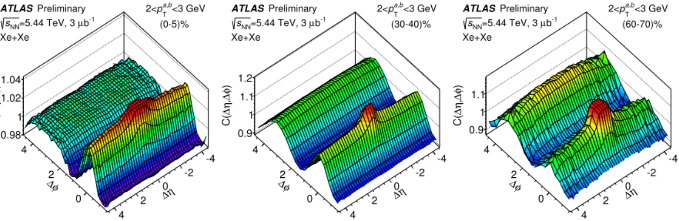
Figure
2shows the
C(∆η,∆φ)for a central (0–5%), a mid-central (30–40%), and a peripheral (60–70%) centrality interval, for 2
< pa,bT <
3 GeV. In all cases a peak is seen in the correlation at
(∆η,∆φ) ∼ (0
,0
). This peak arises from short-range correlations such as resonance decays, or jet-fragmentation. The long- range (large
∆η) correlations are the result of the global anisotropy of the event and are the focus of the study in this analysis.
Figure
3shows the corresponding
C(∆φ)(Eq. (2)) corresponding to the
C(∆η,∆φ)shown in Figure
2.The continuous line is a Fourier fit to the correlation (Eq. (3)) that includes harmonics up to
n=6. The
y-axis limits for the different panels are kept identical so that the modulation in the correlation across thedifferent centralities can be easily compared. It is seen that the modulation in the correlation is smallest
in the most central events (left panel) and increases towards mid-central events reaching a maximum in
∆φ 0 2 4
∆η -4 -2 0 2 4
)φ∆,η∆C(
0.98 1 1.02 1.04
ATLASPreliminary b-1
=5.44 TeV, 3 µ sNN
Xe+Xe
<3 GeV
b , a
pT
2<
(0-5)%
∆φ 0 2 4
∆η -4 -2 0 2 4
)φ∆,η∆C(
0.9 1 1.1 1.2
ATLASPreliminary b-1
=5.44 TeV, 3 µ sNN
Xe+Xe
<3 GeV
b , a
pT
2<
(30-40)%
∆φ 0 2 4
∆η -4 -2 0 2 4
)φ∆,η∆C(
0.9 1 1.1
ATLAS Preliminary b-1
=5.44 TeV, 3 µ sNN
Xe+Xe
<3 GeV
b , a
pT
2<
(60-70)%
Figure 2: Two-particle correlations in∆η−∆φfor 2<pa,b
T <3 GeV. Each panel is a different centrality bin.
φ
∆
0 2 4
)φ∆C(
0.9 1 1.1
ATLAS Preliminary Xe+Xe
b-1
µ
=5.44 TeV, 3 sNN
(0-5)%
|<5 η 2<|∆
<3 GeV
,b a
pT
2<
φ
∆
0 2 4
)φ∆C(
0.9 1 1.1
ATLAS Preliminary Xe+Xe
b-1
µ
=5.44 TeV, 3 sNN
(30-40)%
|<5 η
∆ 2<|
<3 GeV
b , a
pT
2<
φ
∆
0 2 4
)φ∆C(
0.9 1 1.1
ATLAS Preliminary Xe+Xe
b-1
µ
=5.44 TeV, 3 sNN
(60-70)%
|<5 η
∆ 2<|
<3 GeV
b , a
pT
2<
Figure 3: Two-particle correlations in∆φfor|∆η| ∈ (2,5)and 2<pa,b
T <3 GeV. Each panel is a different centrality bin. Also shown is a Fourier fit to the correlation (Eq. (3)) that includes harmonics up ton=6.
φ
∆
0 2 4
)φ∆C(
0.98 1 1.02 1.04
ATLAS Preliminary b-1
=5.44 TeV, 3 µ sNN
Xe+Xe
(0-5)% 2<|∆η|<5
<3 GeV b , a pT 2<
φ
∆
0 2 4
)φ∆C(
1 1.1
ATLAS Preliminary b-1
=5.44 TeV, 3 µ sNN
Xe+Xe
(30-40)% 2<|∆η|<5
<3 GeV b , a pT 2<
φ
∆
0 2 4
)φ∆C(
0.95 1 1.05 1.1
ATLAS Preliminary b-1
=5.44 TeV, 3 µ sNN
Xe+Xe
(60-70)% 2<|∆η|<5
<3 GeV b , a pT 2<
Figure 4: Two-particle correlations in∆φfor|∆η| ∈ (2,5)and 2<pa,b
T <3 GeV. Also shown is a Fourier fit to the correlation (Eq. (3)) that includes harmonicsnup to 6. The individual contribution of the different harmonics to the 2PC are also shown (different colored curves). The individualvn,ncan be identified by the number of peaks in
∆φ, eg. 2 forn=2, etc. Each panel is a different centrality bin.
[GeV]
b
pT
1 10
){2PC}Tp(nv
0 0.1 0.2 0.3
v2
v3
v4
v5 ATLAS Preliminary
b-1
=5.44 TeV, 3 µ sNN
Xe+Xe
<5 GeV
a
pT
0.5<
|<5 η 2<|∆ (0-5)%
[GeV]
b
pT
1 10
){2PC} Tp(nv
0 0.1 0.2 0.3
v2
v3
v4
v5 ATLAS Preliminary
b-1
µ
=5.44 TeV, 3 sNN
Xe+Xe
<5 GeV
a
pT
0.5<
|<5 η
∆ 2<|
(5-10)%
[GeV]
b
pT
1 10
){2PC}Tp(nv
0 0.1 0.2 0.3
v2
v3
v4
v5 ATLASPreliminary
b-1
µ
=5.44 TeV, 3 sNN
Xe+Xe
<5 GeV
a
pT
0.5<
|<5 η
∆ 2<|
(10-20)%
[GeV]
b
pT
1 10
){2PC}Tp(nv
0 0.1 0.2 0.3
v2
v3
v4
ATLAS Preliminary b-1
µ
=5.44 TeV, 3 sNN
Xe+Xe
<5 GeV
a
pT
0.5<
|<5 η
∆ 2<|
(20-30)%
[GeV]
b
pT
1 10
){2PC} Tp(nv
0 0.1 0.2 0.3
v2
v3
v4
ATLAS Preliminary b-1
µ
=5.44 TeV, 3 sNN
Xe+Xe
<5 GeV
a
pT
0.5<
|<5 η
∆ 2<|
(30-40)%
[GeV]
b
pT
1 10
){2PC}Tp(nv
0 0.1 0.2 0.3
v2
v3
v4
ATLASPreliminary b-1
µ
=5.44 TeV, 3 sNN
Xe+Xe
<5 GeV
a
pT
0.5<
|<5 η
∆ 2<|
(40-50)%
[GeV]
b
pT
1 10
){2PC}Tp(nv
0 0.1 0.2 0.3
v2
v3
v4
ATLAS Preliminary b-1
=5.44 TeV, 3 µ sNN
Xe+Xe
<5 GeV
a
pT
0.5<
|<5 η 2<|∆ (50-60)%
[GeV]
b
pT
1 10
){2PC} Tp(nv
0 0.1 0.2 0.3
v2
v3
v4
ATLAS Preliminary b-1
=5.44 TeV, 3 µ sNN
Xe+Xe
<5 GeV
a
pT
0.5<
|<5 η 2<|∆ (60-70)%
[GeV]
b
pT
1 10
){2PC}Tp(nv
0 0.1 0.2 0.3
v2
v3
v4
ATLASPreliminary b-1
=5.44 TeV, 3 µ sNN
Xe+Xe
<5 GeV
a
pT
0.5<
|<5 η 2<|∆ (70-80)%
Figure 5: The pb
T dependence of thevn. Each panel is a different centrality interval. The error bars and bands indicate statistical and systematic uncertainties, respectively. Thev2 values are shown up to 20 GeV. The higher order harmonicsv3andv4are shown up topTof 8 GeV. The harmonicv5is shown only over the 0–20% centrality range and up to 8 GeV.
the 30–40% centrality interval (middle panel) and then decreases for the more peripheral events (right panel). This is the trend of the centrality dependence of most
vn,n, especially the
v2,2. Figure
4shows the same correlation functions but with the
y-axis range expanded to facilitate observing the features ofthe correlation. The Fourier fit is indicated by the thick black line and the contribution of the individual
vn,nare also shown. In the most central (0-5%) collisions the
v2,2-
v4,4are of comparable magnitude.
But in the 30–40% and 60–70% centralities, where the average collision geometry is elliptic, the
v2,2is significantly larger than the other
vn,n(
n≥3). In central events the away-side peak is also much broader due to the comparable magnitude of the higher order harmonics to
v2,2, while in mid-central events the near- and away-side peaks are quite symmetric as the
v2,2dominates. In central and mid-central events, the near-side peak is larger than the away-side peak. However, beyond 60% centrality the away-side peak becomes larger indicating the presence of a large negative
v1,1component. This negative
v1,1component in the peripheral 2PCs arises largely from dijets: while the near-side jet peak is rejected by the
|∆η|>2 cut, the away-side jet moves around in
|∆η|event by event, and cannot be rejected entirely. The presence of the away-side jet produces a large negative
v1,1and also affects the other harmonics. Over this centrality range the
vn,nare biased by dijets especially at higher
pT.
Figure
5shows the
pTdependence of the
vnfor
n=2-5. Each panel is a different centrality interval, and
the results cover the 0–80% centrality range. For the higher-order harmonic
v5, the results are shown over
the 0–20% centrality interval only, beyond which the statistical and systematic errors are too large for a meaningful study of the
pTdependence. For the same reason, results for
v3–v
5are shown only up to
pTof 8 GeV. The
vnincrease at low
pTand reach a maximum between 2–4 GeV and then decrease. For nearly all centralities, the
vnfollow the trend
v2>>
v3> v4 >v5. This hierarchy breaks down in the most central (0-5%) collisions where the
v3at
pT>3 GeV becomes bigger than
v2. These trends are identical to those seen in the
vnmeasurements in Pb+Pb collisions at
√sNN
=2.76 TeV [2] and 5.02 TeV [3]. For peripheral events, at the highest
pTthe even-order
vnagain increase, while the odd-order
vnare suppressed. This increase is due to bias from jets, which dominate the 2PC at high
pTin peripheral events. This is most clearly seen for
v2.
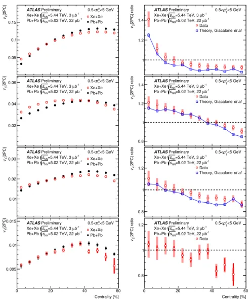
The left panel of Figures
6compares the centrality dependence of the
vnmeasured in the present Xe+Xe analysis with the corresponding Pb+Pb measurements at
√sNN
=5.02 TeV [3]. The comparisons are made for the 0.5–5 GeV
pTinterval. The ratio of the Xe+Xe
vnto the Pb+Pb
vnare shown in the right panels.
For
v2–
v4the ratios are also compared to theoretical predictions from Ref. [4]. The theoretical predictions
are for the 0.3–5 GeV
pTinterval. However the ratio is expected to vary only weakly with
pT, and so
the comparison to the measured
vnin the 0.5–5 GeV
pTinterval should be valid. It is seen that for
v2in
central events, the Xe+Xe values are considerably larger than the Pb+Pb values. This is seen most clearly
from the ratio plots. With decreasing centrality the ratio for
v2decreases faster and becomes smaller than
unity by the 10–15% centrality interval. For more peripheral events the ratio keeps decreasing but at a
smaller rate and becomes roughly 0.9 by the 60–70% centrality. For
v3the Xe+Xe values are larger than
the Pb+Pb values over the 0–30% centrality interval, becoming comparable over the 30–40% centrality
interval and smaller for more peripheral events. In this case the ratio in the 0–5% most central events
is smaller than for
v2, and decreases almost linearly over the 0–70% centrality range. For
v4the Xe+Xe
values are only marginally larger in the 0–5% central events. The ratio for
v4becomes comparable or less
than one by the 5–10% centrality and continues to decrease for more peripheral events. For
v5the Xe+Xe
values are smaller throughout.
Centrality [%]
0 20 40 60
{2PC}2v
0.05 0.1
0.15 Pb+Pb
Xe+Xe b-1
=5.02 TeV, 22 µ sNN
Pb+Pb ATLASPreliminary
b-1
=5.44 TeV, 3 µ sNN
Xe+Xe
<5 GeV
b
pT
0.5<
Centrality [%]
0 20 40 60
ratio{2PC}2v
1 1.2
1.4 Pb+Pb sNN=5.02 TeV, 22 µb-1 Data
et al Theory, Giacalone ATLASPreliminary
b-1
=5.44 TeV, 3 µ sNN
Xe+Xe
<5 GeV
b
pT
0.5<
Centrality [%]
0 20 40 60
{2PC}3v
0.02 0.04 0.06
Pb+Pb Xe+Xe b-1
=5.02 TeV, 22 µ sNN
Pb+Pb ATLASPreliminary
b-1
=5.44 TeV, 3 µ sNN
Xe+Xe
<5 GeV
b
pT
0.5<
Centrality [%]
0 20 40 60
ratio{2PC}3v
0.8 1 1.2 1.4
b-1
=5.02 TeV, 22 µ sNN
Pb+Pb
Data
et al Theory, Giacalone ATLASPreliminary
b-1
=5.44 TeV, 3 µ sNN
Xe+Xe
<5 GeV
b
pT
0.5<
Centrality [%]
0 20 40 60
{2PC}4v
0.01 0.02 0.03
Pb+Pb Xe+Xe b-1
=5.02 TeV, 22 µ sNN
Pb+Pb ATLASPreliminary
b-1
=5.44 TeV, 3 µ sNN
Xe+Xe
<5 GeV
b
pT
0.5<
Centrality [%]
0 20 40 60
ratio{2PC}4v
0.8 1 1.2
b-1
=5.02 TeV, 22 µ sNN
Pb+Pb
Data
et al Theory, Giacalone ATLASPreliminary
b-1
=5.44 TeV, 3 µ sNN
Xe+Xe
<5 GeV
b
pT
0.5<
Centrality [%]
0 20 40 60
{2PC}5v
0.005 0.01 0.015
Pb+Pb Xe+Xe b-1
=5.02 TeV, 22 µ sNN
Pb+Pb ATLASPreliminary
b-1
=5.44 TeV, 3 µ sNN
Xe+Xe
<5 GeV
b
pT
0.5<
Centrality [%]
0 20 40 60
ratio{2PC}5v
0.8 1 1.2
b-1
=5.02 TeV, 22 µ sNN
Pb+Pb
Data ATLASPreliminary
b-1
=5.44 TeV, 3 µ sNN
Xe+Xe
<5 GeV
b
pT
0.5<
Figure 6: Left panels: comparisons of the centrality dependence of the vn measured in Pb+Pb collisions at
√sNN=5.02 TeV to the present Xe+Xe measurements. The plots are for the 0.5-5 GeVpTinterval. From top to
bottom each row corresponds to a differentn. The right panels show the ratio of the Xe+Xevnto the Pb+Pbvn. The ratios are compared to theoretical predictions 0.3–5 GeVpTinterval from Ref. [4]. The error bars and bands indicate statistical and systematic uncertainties, respectively.