Measurement of the Lund jet plane using charged particles with the ATLAS detector from 13 TeV proton–proton collisions

A TLAS-CONF-2019-035 25 July 2019

ATLAS CONF Note

ATLAS-CONF-2019-035

July 24, 2019

Measurement of the Lund jet plane using charged particles with the ATLAS detector from 13 TeV

proton–proton collisions

The ATLAS Collaboration

The prevalence of hadronic jets at the Large Hadron Collider (LHC) requires that a deep understanding of jet formation and structure must be achieved in order to reach the highest levels of experimental and theoretical precision. There have been many measurements of jet substructure at the LHC and previous colliders, but the targeted observables mix physical effects from various origins. Based on a new proposal to factorize physical effects, this note presents a double-differential cross section measurement of the Lund jet plane using 139 fb

of

√ s =13 TeV pp data collected with the ATLAS detector. The measurement uses charged particles to achieve a fine angular resolution and is corrected for acceptance and detector effects. Several parton shower Monte Carlo models are compared with the data.

Multiple parton shower Monte Carlo simulations are compared with data to study the modeling of various physical effects across the plane.

© 2019 CERN for the benefit of the ATLAS Collaboration.

Reproduction of this article or parts of it is allowed as specified in the CC-BY-4.0 license.

High energy quarks and gluons are ubiquitous in collisions at the Large Hadron Collider (LHC), but cannot be directly observed due to the confining nature of the strong force: instead, collimated jets of particles emerge from quark and gluon scattering. The internal substructure of a jet encodes information about the originating parton. Jet dynamics are governed by Quantum Chromodynamics (QCD) with one coupling constant called α

. In the soft gluon (‘eikonal’) picture of jet formation, a quark or gluon radiates a haze of relatively low energy and statistically-independent gluons [1, 2]. QCD is nearly scale-invariant, and so this emission pattern is approximately uniform in the Lund plane [3]: a two-dimensional space spanned by ln ( 1 /z) and ln ( 1 /θ) , where z is the momentum fraction of the (relatively soft) emitted gluon relative to the primary quark or gluon and θ is the opening angle of the emission. This description can be extended to higher orders in QCD and has served as the basis for many calculations of jet substructure observables (see Refs. [4–7]).

The Lund plane is a powerful representation to provide insight and predictions for the entire radiation pattern within jets. However, because it is constructed from quarks and gluons within a particular theoretical framework, it is not observable due to the effects of confinement. A recent proposal [8] described an approach to approximate the radiation from a primary high-energy quark or gluon by declustering jets. Jets are defined in-part by a clustering algorithm; the most popular algorithms sequentially combine pairs of proto-jets to produce a set of jets from an initial set of jet constituents [9]. The proposal from Ref. [8]

prescribes the reclustering of a jet’s constituents using the Cambridge/Aachen (C/A) [10, 11] recombination algorithm, which imposes an angularly-ordered hierarchy on the jet’s clustering history. Then, by traversing the C/A clustering history in reverse while following the harder proto-jet (i.e., by following the primary clutering sequence), one can approximate the Lund plane by treating the proto-jet pair at each step in the sequence as a proxy for an emission (represented by the softer proto-jet) and the jet core (represented by the harder proto-jet) in the original theoretical depiction. For each proto-jet pair, at each step in the C/A declustering sequence, an entry may be made in the approximate Lund plane (henceforth, the ‘Lund jet plane’) by defining a coordinate pair of ‘Lund jet plane observables’ ( log ( 1 /z), log (R/∆R)) with

z = p

T

p

T

+ p

T

and ∆R

= ( y

− y

)

+ (φ

− φ

)

,

where p

is the transverse momentum

, y is the rapidity, and R is the radius parameter used during jet reconstruction. Using this approach, individual jets are represented as a set of points within the Lund jet plane, and ensembles of jets may be studied by measuring the double-differential cross section in this space.

The structure of emissions, which may themselves be composite objects, is not considered in this analysis.

To leading-logarithmic (LL) order, the average density of emissions within the primary Lund jet plane is uniform [8]:

1 N

d

N

dzd∆R ∝ 1

z 1

∆R ,

where n

is the jet multiplicity. This picture of the plane in terms of z and ∆R is selected in order to cleanly factorise the momentum and angular measurements, although other depictions drawn in terms of e.g. k

= zθ are also valid representations.

This note presents a two-dimensional differential cross section measurement of the Lund jet plane which is corrected for distortions due to detector effects, using 139 fb

of

√ s = 13 TeV pp collision data

1

ATLAS uses a right-handed coordinate system with its origin at the nominal interaction point (IP) in the center of the detector

and the z-axis along the beam pipe. The x-axis points from the IP to the center of the LHC ring, and the y -axis points

upward. Cylindrical coordinates ( r , φ ) are used in the transverse plane, φ being the azimuthal angle around the beam pipe. The

pseudorapidity is defined in terms of the polar angle as η = − ln tan ( polar angle / 2 ) .

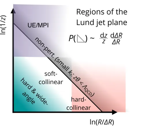
collected by the ATLAS detector during Run 2 of the LHC. In contrast to previous measurements of jet substructure, in the context of QCD, the radiation from different physical processes such as initial state radiation, underlying event (UE), hadronization, and perturbative emissions are factorized as illustrated in Figure 1. As different regions are dominated by factorised processes, the differential cross section of the Lund jet plane can be simultaneously useful for tuning non-perturbative models and for constraining advanced parton shower (PS) Monte Carlo programs [12–15] and state-of-the-art QCD calculations of jet substructure [16–21] which have so far only been constrained by the jet mass [22, 23] (which is itself a diagonal ray in the Lund jet plane: ln 1 /z ∼ ln m

/p

T

− 2 ln R/∆R ). Furthermore, the number of emissions within regions of the Lund jet plane is calculable within QCD and provides provably optimal discrimination between quark and gluon jets [5].

ln(R/∆R)

ln(1/ z )

har d &

wid e- angle

soft- collinear

hard- collinear UE/MPI

Regions of the Lund jet plane

P( ) ~ ^dz _z ^d∆R _∆R

non -per

t. (s ma ll k _t : z θ <

Λ _QCD )

Figure 1: Schematic representation of the Lund jet plane, indicating the source of emissions which typically populate each region. Areas dominated by radiation in QCD originating from the underlying event (UE) and multi-parton interactions (MPI), soft-collinear splittings, hard-collinear splittings and hard, wide-angle radiation are indicated.

The ‘non-perturbative’ region lies above the diagonal band, and is populated by emissions with small k

∼ zθ .

The ATLAS detector [24–26] is a general-purpose particle detector which provides nearly 4 π coverage in

solid angle. The inner tracking detector (ID) is inside a 2 T magnetic field and is designed to measure

charged-particle trajectories up to |η| = 2 . 5. The innermost component of the ID is a pixelated silicon

detector with fine granularity that is able to resolve ambiguities inside the dense hit environment of jet

cores [27], surrounded by silicon strip and transition radiation tracking detectors. Beyond the ID are

electromagnetic and hadronic calorimeters, from which topologically-connected clusters of cells [28] are clustered to form jets with the anti- k

algorithm with radius parameter R = 0 . 4 [29, 30]. The energy scale of these jets is calibrated so that on average, the detector-level jet energy is the same as that of the corresponding particle-level jets [31]. The rate of jet production is too large to record every multijet event;

therefore, only jets with a large enough p

are saved as part of the ATLAS two-level trigger system [32, 33].

Events which are used in this measurement are selected online using a set of single-jet triggers which are fully efficient throughout the Run 2 dataset for jets used in this analysis. A well-balanced dijet system is required to be present, where the leading jet satisfies p

T

> 500 GeV and the system satisfies p

T

< 1 . 5 × p

T

. Both jets must be within |η | < 2 . 1 in order to ensure that they are completely within the ID acceptance. Approximately 115 million reconstructed jets satisfy these selection criteria.

Particle-level charged hadrons and their reconstructed tracks are used for this measurement because individual particle trajectories can be precisely identified with the ID. As the Lund jet plane observables are dimensionless and isospin is an approximate symmetry of the strong force, the difference between the considered observables constructed using either all particles or charged particles following the analysis selections is small. ID tracks within ∆R = 0 . 4 of the axis of selected jets are used to construct the Lund jet plane observables: tracks associated with each jet are clustered using the C/A algorithm, and the plane is populated by iteratively declustering the clustering history. These tracks are required to have a p

> 0 . 5 GeV, to be associated with the primary vertex of the event, and to satisfy “loose”

reconstruction quality criteria [34]. The measured Lund jet plane cross section is presented with 21 bins in ln ( 1 /z) between ln ( 1 / 0 . 5 ) and 9 . 4 × ln ( 1 / 0 . 5 ) and 15 bins in ln (R/∆R) between 0 . 0 and 5 . 0. The log (R/∆R) range is set to span the distance scale between the jet radius (log ( 0 . 4 / 0 . 4 ) = 0) and a minimum scale which is comparable to the pixel pitch (log ( 0 . 4 / 5 ) ∼ 50 microns / 33 mm ∼ 0 . 0015 ). The maximum z is 0.5 and the minimum is 500 MeV /p

T

, which is 0 . 001 for jets at the threshold of p

T

= 500 GeV.

A set of dijet events are simulated in order to perform the unfolding as well as to compare with the corrected data. The nominal set is simulated using Pythia 8.186 [35, 36] with the NNPDF2.3 LO [37] set of parton distribution functions (PDFs), a p

-ordered PS, Lund string hadronization [38, 39], and the A14 set of tuned parameters (tune) [40]. Additional sets include: two sets of Pythia 8.230 [41] with the NNPDF2.3 LO PDF set and the A14 tune that are either using the Pythia LO matrix elements or NLO matrix elements from Powheg [42–45], Sherpa 2.1.1 [46] with the CT10LO PDF set, a p

-ordered PS [47], and a cluster-based hadronization model [48], two sets of Sherpa 2.2.5 with the CT14NNLO PDF set [49]

and either a cluster hadronization model or the Lund string model, and two sets of Herwig 7.1.3 [15, 50, 51] with the MMHT2014NLO PDF set [52] and either the default angularly-ordered PS or a dipole PS and a cluster hadronization [48]. Additional details of these samples may be found in Ref. [53]. The Pythia 8.186 and Sherpa 2.1.1 events are passed through the ATLAS detector simulation [54] based on Geant 4 [55]. The effect of multiple pp interactions in the same and neighbouring bunch crossings (‘pileup’) is modelled in these samples by overlaying minimum-bias pp collisions, which are generated using Pythia 8 with the A3 set of tuned parameters [56] and NNPDF2.3 LO PDF set. The distribution of pileup is reweighted to match that of the data.

Selected data are unfolded in order to correct for detector bias, resolution, and acceptance effects using an Iterative Bayesian (IB) technique [57] and four iterations, as implemented in the RooUnfold framework [58].

The number of iterations was chosen to minimize the total uncertainty. The unfolding procedure corrects the

Lund jet plane constructed from detector-level objects to particle-level, where jets and charged particles are

defined similarly to detector-level: jets are clustered using the same anti- k

algorithm with detector-stable

( cτ > 10 mm) hard-scatter hadrons as inputs. The same kinematic requirements are imposed on the

particle-level jet as for detector-level jets; charged particles with p

> 0 . 5 GeV within ∆R < 0 . 4 of the particle-level jets are used to populate the particle-level Lund jet plane.

Emissions at detector-level and particle-level are matched in η − φ to construct the response matrix. This matching is unique, with the closest match within ∆R = 0 . 1 taking precedence. Unmatched emissions from tracks not due to a single charged particle (detector-level) and from non-reconstructed charged particles (particle-level) are accounted for with acceptance and efficiency corrections, before and after the response matrix portion of the IB method. These corrections are about 20% for the lower left quadrant of the plane and increase to 90% in the most collinear bins and to 50% in the lowest z bins. Despite the large corrections, the correction factors are robust to all systematic variations within 10%, as described below. The matching procedure follows the order of the C/A declustering, starting from the widest-angle emissions and iterating towards the jet core. An uncertainty on this matching procedure is established by repeating the unfolding procedure and iterating through the C/A declustering sequence in reverse, and taking the difference in the unfolded result as an uncertainty. This uncertainty is less than 1% except in the highest log ( R/∆R) bin.

For matched emissions, the log ( 1 /z) and log (R/∆R) migrations are largely independent of each other.

Furthermore, since the differential distribution is slowly varying across the Lund jet plane, the purity and efficiencies are approximately the same. The log (R/∆R) migrations in a given log ( 1 /z) bin are about 50%

for the smallest opening angles and decrease to under 10% for the widest angles. The log ( 1 /z) migrations decrease from about 50% for the softest emissions to about 20% for the hardest ones, with some degradation for the softest emissions at small opening angles. Migrations for both observables are nearly symmetric except for log (R/∆R) & 3, where harder to resolve small opening angles are asymmetrically measured as larger ones and . 10% of the time emissions are mis-matched between particle-level and detector-level and therefore measured with the wrong log ( 1 /z) . While the log (R/∆R) migrations are nearly the same when log ( 1 /z) migrates by one bin, the log ( 1 /z) migrations increase by about 30% when log (R/∆R) migrates by one bin.

The unfolded distribution is normalized by the number of jets that pass the event selection, and so this measurement is made insensitive to the total jet cross section. Following normalization, the integral of the Lund jet plane is the average number of emissions within the fiducial region studied.

Systematic uncertainties on the measured cross section distribution may be broadly classified as one of two types: experimental uncertainties related to the measurement and reconstruction of the objects used to perform this measurement, and theoretical uncertainties related to the modeling of jet fragmentation.

These uncertainties are evaluated by modifying some aspect of the unfolding procedure and taking the difference with respect to the nominal result.

Experimental uncertainties from various sources are considered and found to be comparable to those arising from theoretical sources in some regions of the Lund jet plane. Uncertainties on the jet energy scale and resolution are measured using several simulation-based and in situ techniques [31]. These uncertainties cause the migration of jets into or out of the fiducial acceptance which causes an uncertainty on the measured observables to typically be above 3%, reaching up to 7% in certain regions of the plane.

Uncertainties related to the track reconstruction both for isolated tracks and those within dense environments are considered, which modify the measured p

of individual tracks or remove them completely [27, 59].

These uncertainties are typically small, contributing less than a half-percent to the total uncertainty.

A data-driven non-closure uncertainty is determined by unfolding the nominal particle-level spectrum following a reweighting based on the corresponding simulated detector-level spectrum and the data [60].

This uncertainty is less than 1% except for the smallest opening angles, where it can reach 5%. Other

experimental uncertainties related to the stability of the measurement to the effects of pileup are considered, and are found to be negligible.

Theoretical uncertainties predominantly arise due to the limited accuracy of jet fragmentation modelling.

Variations in jet fragmentation can impact the response matrix as well as the unfolding correction factors.

The impact of this uncertainty on the measurement is evaluated by repeating the unfolding procedure with variations of the Monte Carlo generators used. As Pythia 8.186 is used to perform the nominal unfolding, the impact of constructing the unfolding matrix using simulated Sherpa 2.2.1 dijet events is evaluated. This alternative matrix is used to unfold the nominal reconstructed Pythia 8.186 sample, and differences between these results and the nominal particle-level Pythia 8.186 Lund jet plane are taken as an uncertainty, which is typically between 1–10% depending on the considered region (larger in the soft-collinear) and is the largest single source of uncertainty associated with this measurement.

The measured Lund jet plane following the unfolding procedure is shown in Figure 2. A triangular region is populated uniformly by perturbative emissions within the ensemble of jets. A large number of emissions can be found at the transition to the non-perturbative regime, as α

( k

) is enhanced for small values of k

. Non-perturbative emissions beyond this region, for which k

∼ Λ

, are suppressed. The average number of emissions in the measured region (integral of the Lund jet plane) is measured to be 7.75 emissions while the corresponding value for Pythia 8.186 is 8.13 emissions and for Sherpa 2.2.1 is 7.51 emissions. A total uncertainty of ± 0 . 11 is associated with this measured value, found by propagating all systematic uncertainties from the unfolded measurement in an uncorrelated and symmetrized manner. The associated statistical uncertainty on this value is negligible. While this bracketing of the data by Pythia 8.186 and Sherpa 2.2.1 in the particle multiplicity inside jets has been observed before [61], it has never been decomposed into a perturbative and non-perturbative component.

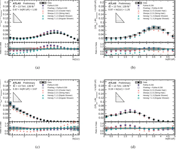
Figure 3 shows data from four selected horizontal and vertical slices through the Lund jet plane. These data are compared to predictions from multiple Monte Carlo generators. While no one prediction describes the data in all regions, the Herwig 7.1.3 angularly-ordered prediction provides the best description across most of the plane. The Pythia 8.186 and Sherpa 2.2.1 predictions are not shown, but are consistent with the Pythia 8.230 and Sherpa 2.2.5 (Cluster Had.) predictions, respectively. The differences between the shower algorithms implemented in Herwig 7.1.3 are present only at low values of z∆R while the differences between the hadronization algorithms implemented in Sherpa 2.2.5 are present mostly at large z∆R . Similarly the Pythia and Sherpa +string predictions are nearly the same in the high z∆R region. Since the Lund jet plane is reconstructed for small-radius jets, there is no difference between the Powheg+Pythia and Pythia predictions. These observations demonstrate that the Lund jet plane is able to isolate various effects and can therefore provide useful input to both perturbative and non-perturbative model development and tuning.

In summary, a measurement of the substructure of jets initiated by quarks and gluons as represented by

the Lund jet plane is reported, which was performed in 139 fb

of LHC pp collisions recorded by the

ATLAS detector during Run 2 of the LHC. This measurement is performed on an inclusive selection of dijet

events, with a leading jet p

> 500 GeV. Selected jets are reconstructed from topological clusters using

the anti- k

algorithm with R = 0 . 4, and their associated charged-particle tracks are used to construct the

observables of interest. The measured data are presented as an unfolded double-differential cross section,

and compared to several Monte Carlo generators. The average number of emissions entering the region

of the Lund jet plane is measured to be 7 . 75 ± 0 . 11. The measured data disagree with predictions from

simulation throughout the measured parameter space, and are a first demonstration of the Lund jet plane’s

potential to isolate various effects and to provide useful input to both perturbative and non-perturbative

model development and tuning.

0 0.01 0.02 0.03 0.04 0.05 0.06 0.07 0.08 2

) R ∆ / R ) d ln( z d ln(1/ / N d 1/N

0 0.5 1 1.5 2 2.5 3 3.5 4 4.5 5

)

∆ R / R ln(

1 2 3 4 5 6

) z ln(1/

ATLAS Preliminary s = 13 TeV, 139 fb

−2

10

−1

10 )

p +

p / (

p = z

−2 1

10

10

(emission, core)

∆ R =

∆ R

0 0.05 0.1 0.15 0.2 0.25 0.3 0.35

Relative Uncertainty

0 0.5 1 1.5 2 2.5 3 3.5 4 4.5 5

)

∆ R / R ln(

1 2 3 4 5 6

) z ln(1/

ATLAS Preliminary s = 13 TeV, 139 fb

−2

10

−1

10 )

p +

p / (

p = z

−2 1

10

10

(emission, core)

∆ R =

∆ R

Figure 2: Top: The Lund jet plane as measured using jets in 13 TeV pp collision data, corrected to particle-level.

The inner set of axes indicate the coordinates of the Lund jet plane itself, while the outer set indicate corresponding

values of z and ∆R . Bottom: The total relative uncertainty (experimental, statistical and related to Monte Carlo

modeling effects) as a function of the Lund jet plane observables.

1 2 3 4 5 6 ) z ln(1/

0.02 0.04 0.06 0.08 0.1 0.12 0.14 0.16 0.18 0.2 )z / d ln(1/emissions) dNjets(1/N

ATLAS Preliminary = 13 TeV, 139 fb-1

s

) < 1.00

∆R / R 0.67 < ln(

Data Pythia 8.230 Powheg + Pythia 8.230 Sherpa 2.2.5 (Cluster Had.) Sherpa 2.2.5 (String Had.) Herwig 7.1.3 (Dipole Shower) Herwig 7.1.3 (Angular Shower)

1 2 3 4 5 6

) z ln(1/

0.6 0.81 1.2 1.4

Ratio to Data

(a)

0 0.5 1 1.5 2 2.5 3 3.5 4 4.5 5

)

∆R / R ln(

0.02 0.04 0.06 0.08 0.1 0.12 0.14 0.16 0.18 0.2 )R∆/R / d ln(emissions) dNjets(1/N

ATLAS Preliminary = 13 TeV, 139 fb-1

s

) < 1.25 z 0.97 < ln(1/

Data Pythia 8.230 Powheg + Pythia 8.230 Sherpa 2.2.5 (Cluster Had.) Sherpa 2.2.5 (String Had.) Herwig 7.1.3 (Dipole Shower) Herwig 7.1.3 (Angular Shower)

0 0.5 1 1.5 2 2.5 3 3.5 4 4.5 5

)

∆R / R ln(

0.6 0.81 1.2 1.4

Ratio to Data

(b)

1 2 3 4 5 6

) z ln(1/

0.02 0.04 0.06 0.08 0.1 0.12 0.14 0.16 0.18 0.2 )z / d ln(1/emissions) dNjets(1/N

ATLAS Preliminary = 13 TeV, 139 fb-1

s

) < 3.67

∆R / R 3.33 < ln(

Data Pythia 8.230 Powheg + Pythia 8.230 Sherpa 2.2.5 (Cluster Had.) Sherpa 2.2.5 (String Had.) Herwig 7.1.3 (Dipole Shower) Herwig 7.1.3 (Angular Shower)

1 2 3 4 5 6

) z ln(1/

0.6 0.81 1.2 1.4

Ratio to Data

(c)

0 0.5 1 1.5 2 2.5 3 3.5 4 4.5 5

)

∆R / R ln(

0.02 0.04 0.06 0.08 0.1 0.12 0.14 0.16 0.18 0.2 )R∆/R / d ln(emissions) dNjets(1/N

ATLAS Preliminary = 13 TeV, 139 fb-1

s

) < 3.47 z 3.19 < ln(1/

Data Pythia 8.230 Powheg + Pythia 8.230 Sherpa 2.2.5 (Cluster Had.) Sherpa 2.2.5 (String Had.) Herwig 7.1.3 (Dipole Shower) Herwig 7.1.3 (Angular Shower)

0 0.5 1 1.5 2 2.5 3 3.5 4 4.5 5

)

∆R / R ln(

0.6 0.81 1.2 1.4

Ratio to Data

(d)

Figure 3: Representative horizontal and vertical slices through the Lund jet plane. Unfolded data are compared to

particle-level simulation from several Monte Carlo generators. The uncertainty band includes all sources of systematic

and statistical uncertainty. The inset triangle illustrates which slice of the plane is depicted: 0 . 67 < ln (R/∆R) < 1 . 00

(a), 0 . 97 < ln ( 1 /z) < 1 . 25 (b), 3 . 33 < ln (R/∆R) < 3 . 67 (c), and 3 . 19 < ln ( 1 /z) < 3 . 47 (d).

Appendix

0 0.01 0.02 0.03 0.04 0.05 0.06 0.07 0.08 2 ) R ∆ / R ) d ln( z d ln(1/ / N d 1/N emissions jets

0 0.5 1 1.5 2 2.5 3 3.5 4 4.5 5

)

∆ R / R ln(

1 2 3 4 5 6

) z ln(1/

ATLAS Simulation Preliminary s = 13 TeV, 139 fb

−2

10

−1

10 ) core T p + emission T p / ( emission T p = z

−2 1

10

10

(emission, core)

∆ R =

∆ R

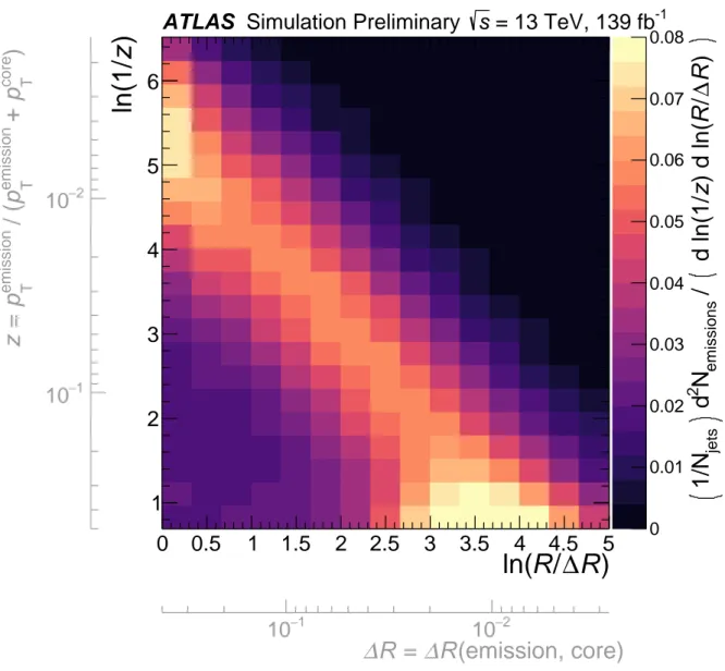
Figure 4: The Lund jet plane as simulated by the Pythia v8.186 Monte Carlo generator. corrected to particle-level.

The inner set of axes indicate the coordinates of the Lund jet plane itself, while the outer set indicate corresponding

values of z and ∆R .

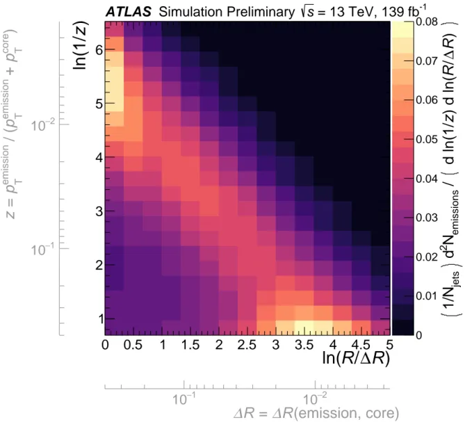
0 0.01 0.02 0.03 0.04 0.05 0.06 0.07 0.08

) R ∆ / R ) d ln( z d ln(1/ / emissions N 2 d jets 1/N

0 0.5 1 1.5 2 2.5 3 3.5 4 4.5 5

)

∆ R / R ln(

1 2 3 4 5 6

) z ln(1/

ATLAS Simulation Preliminary s = 13 TeV, 139 fb

−2

10

−1

10 ) core T p + emission T p / ( emission T p = z

−2 1

10

10

(emission, core)

∆ R =

∆ R

Figure 5: The Lund jet plane as simulated by the Sherpa v2.1.1 Monte Carlo generator. corrected to particle-level.

The inner set of axes indicate the coordinates of the Lund jet plane itself, while the outer set indicate corresponding

values of z and ∆R .

0 0.5 1 1.5 2 2.5 3 3.5 4 4.5 5

∆ R) ln(R/

0 1 2 3 4 5 ln(1/z) 6

Particle-level Emission Detector-level Emission

Simulation Preliminary ATLAS

Pythia 8 Lund Plane Event Display

Figure 6: A set of detector- and truth-level emissions in the Lund jet plane from a single jet. Due to the angular

ordering of the Cambridge/Aachen declustering procedure, markers are filled from left (wide-angle) to right (collinear)

in this figure.

References

[1] J. Gatheral, Exponentiation of eikonal cross sections in nonabelian gauge theories, Phys. Lett. B 133 (1983) 90 (cit. on p. 2).

[2] J. Frenkel and J.C. Taylor, Non-abelian eikonal exponentiation, Nucl. Phys. B 246 (1984) 231 (cit. on p. 2).

[3] B. Andersson, G. Gustafson, L. Lönnblad, and U. Pettersson, Coherence Effects in deep inelastic scattering, Z. Phys. C43 (1989) 625 (cit. on p. 2).

[4] M. Dasgupta, A. Fregoso, S. Marzani, and G. P. Salam, Towards an understanding of jet substructure, JHEP 09 (2013) 029, arXiv: 1307.0007 [hep-ph] (cit. on p. 2).

[5] C. Frye, A. J. Larkoski, J. Thaler, and K. Zhou, Casimir Meets Poisson: Improved Quark/Gluon Discrimination with Counting Observables, JHEP 09 (2017) 083, arXiv: 1704.06266 [hep-ph]

(cit. on pp. 2, 3).

[6] M. Dasgupta, F. A. Dreyer, K. Hamilton, P. F. Monni, and G. P. Salam, Logarithmic accuracy of parton showers: a fixed-order study, JHEP 09 (2018) 033, arXiv: 1805.09327 [hep-ph] (cit. on p. 2).

[7] G. P. Salam, L. Schunk, and G. Soyez, Dichroic subjettiness ratios to distinguish colour flows in boosted boson tagging, JHEP 03 (2017) 022, arXiv: 1612.03917 [hep-ph] (cit. on p. 2).

[8] F. A. Dreyer, G. P. Salam, and G. Soyez, The Lund jet plane, JHEP 12 (2018) 064, arXiv: 1807.04758 [hep-ph] (cit. on p. 2).

[9] G. P. Salam, Towards jetography, Eur. Phys. J. C 67 (2010) 637, arXiv: 0906.1833 [hep-ph]

(cit. on p. 2).

[10] Y. L. Dokshitzer, G. D. Leder, S. Moretti, and B. R. Webber, Better jet clustering algorithms, JHEP 08 (1997) 001, arXiv: hep-ph/9707323 [hep-ph] (cit. on p. 2).

[11] M. Wobisch and T. Wengler, “Hadronization corrections to Jet Cross-Sections in Deep-Inelastic scattering,” Monte Carlo generators for HERA physics. Proceedings, Workshop, Hamburg, Germany, 1998-1999, (1998) 270, arXiv: hep-ph/9907280 [hep-ph] (cit. on p. 2).

[12] N. Fischer, S. Prestel, M. Ritzmann, and P. Skands, VINCIA for hadron colliders, Eur. Phys. J. C 76 (2016) 589, arXiv: 1605.06142 [hep-ph] (cit. on p. 3).

[13] S. Höche and S. Prestel, The midpoint between dipole and parton showers, Eur. Phys. J. C 75 (2015) 461, arXiv: 1506.05057 [hep-ph] (cit. on p. 3).

[14] Z. Nagy and D. E. Soper, Effects of subleading color in a parton shower, JHEP 07 (2015) 119, arXiv: 1501.00778 [hep-ph] (cit. on p. 3).

[15] J. Bellm et al., Herwig 7.0/Herwig++ 3.0 release note, Eur. Phys. J. C 76 (2016) 196, arXiv:

1512.01178 [hep-ph] (cit. on pp. 3, 4).

[16] C. Frye, A. J. Larkoski, M. D. Schwartz, and K. Yan, Factorization for groomed jet substructure beyond the next-to-leading logarithm, JHEP 07 (2016) 064, arXiv: 1603.09338 [hep-ph] (cit. on p. 3).

[17] C. Frye, A. J. Larkoski, M. D. Schwartz, and K. Yan, Precision physics with pile-up insensitive observables, (2016), arXiv: 1603.06375 [hep-ph] (cit. on p. 3).

[18] S. Marzani, L. Schunk, and G. Soyez, A study of jet mass distributions with grooming, JHEP 07

(2017) 132, arXiv: 1704.02210 [hep-ph] (cit. on p. 3).

[19] S. Marzani, L. Schunk, and G. Soyez, The jet mass distribution after Soft Drop, Eur. Phys. J. C 78 (2018) 96, arXiv: 1712.05105 [hep-ph] (cit. on p. 3).

[20] Z.-B. Kang, K. Lee, X. Liu, and F. Ringer, Soft drop groomed jet angularities at the LHC, Phys.

Lett. B 793 (2019) 41, arXiv: 1811.06983 [hep-ph] (cit. on p. 3).

[21] Z.-B. Kang, K. Lee, X. Liu, and F. Ringer, The groomed and ungroomed jet mass distribution for inclusive jet production at the LHC, JHEP 10 (2018) 137, arXiv: 1803.03645 [hep-ph] (cit. on p. 3).

[22] ATLAS Collaboration, Measurement of the Soft-Drop Jet Mass in pp Collisions at

√ s = 13 TeV with the ATLAS detector, Phys. Rev. Lett. 121 (2018) 092001, arXiv: 1711.08341 [hep-ex] (cit. on p. 3).

[23] CMS Collaboration, Measurements of the differential jet cross section as a function of the jet mass in dijet events from proton–proton collisions at

√ s = 13 TeV, JHEP 11 (2018) 113, arXiv: 1807.05974 [hep-ex] (cit. on p. 3).

[24] ATLAS Collaboration, The ATLAS Experiment at the CERN Large Hadron Collider, JINST 3 (2008) S08003 (cit. on p. 3).

[25] ATLAS Collaboration, ATLAS Insertable B-Layer Technical Design Report, ATLAS-TDR-19, 2010, url: https://cds.cern.ch/record/1291633 (cit. on p. 3), Addendum: ATLAS-TDR-19-ADD- 1, 2012, url: https://cds.cern.ch/record/1451888 .

[26] B. Abbott et al., Production and integration of the ATLAS Insertable B-Layer, JINST 13 (2018) T05008, arXiv: 1803.00844 [physics.ins-det] (cit. on p. 3).

[27] ATLAS Collaboration, Performance of the ATLAS track reconstruction algorithms in dense environments in LHC Run 2, Eur. Phys. J. C 77 (2017) 673, arXiv: 1704.07983 [hep-ex] (cit. on pp. 3, 5).

[28] ATLAS Collaboration, Topological cell clustering in the ATLAS calorimeters and its performance in LHC Run 1, Eur. Phys. J. C 77 (2017) 490, arXiv: 1603.02934 [hep-ex] (cit. on p. 4).

[29] M. Cacciari, G. P. Salam, and G. Soyez, The anti- k

jet clustering algorithm, JHEP 04 (2008) 063, arXiv: 0802.1189 [hep-ph] (cit. on p. 4).

[30] M. Cacciari, G. P. Salam, and G. Soyez, FastJet user manual, Eur. Phys. J. C 72 (2012) 1896, arXiv:

1111.6097 [hep-ph] (cit. on p. 4).

[31] ATLAS Collaboration, Jet energy scale measurements and their systematic uncertainties in proton–

proton collisions at

√ s = 13 TeV with the ATLAS detector, Phys. Rev. D 96 (2017) 072002, arXiv:

1703.09665 [hep-ex] (cit. on pp. 4, 5).

[32] ATLAS Collaboration, Performance of the ATLAS trigger system in 2015, Eur. Phys. J. C 77 (2017) 317, arXiv: 1611.09661 [hep-ex] (cit. on p. 4).

[33] ATLAS Collaboration, The performance of the jet trigger for the ATLAS detector during 2011 data taking, Eur. Phys. J. C 76 (2016) 526, arXiv: 1606.07759 [hep-ex] (cit. on p. 4).

[34] ATLAS Collaboration, Early Inner Detector Tracking Performance in the 2015 Data at

√ s = 13 TeV, ATL-PHYS-PUB-2015-051, 2015, url: https://cds.cern.ch/record/2110140 (cit. on p. 4).

[35] T. Sjöstrand, S. Mrenna, and P. Z. Skands, PYTHIA 6.4 Physics and Manual, JHEP 05 (2006) 026, arXiv: hep-ph/0603175 [hep-ph] (cit. on p. 4).

[36] T. Sjöstrand, S. Mrenna, and P. Z. Skands, A brief introduction to PYTHIA 8.1, Comput. Phys.

Commun. 178 (2008) 852, arXiv: 0710.3820 [hep-ph] (cit. on p. 4).

[37] R. D. Ball et al., Parton distributions with LHC data, Nucl. Phys. B 867 (2013) 244 (cit. on p. 4).

[38] B. Andersson, G. Gustafson, G. Ingelman, and T. Sjöstrand, Parton Fragmentation and String Dynamics, Phys. Rept. 97 (1983) 31 (cit. on p. 4).

[39] T. Sjöstrand, Jet fragmentation of multiparton configurations in a string framework, Nucl. Phys. B 248 (1984) 469 (cit. on p. 4).

[40] ATLAS Collaboration, ATLAS Pythia 8 tunes to 7 TeV data, ATL-PHYS-PUB-2014-021, 2014, url:

https://cds.cern.ch/record/1966419 (cit. on p. 4).

[41] T. Sjöstrand et al., An Introduction to PYTHIA 8.2, Comput. Phys. Commun. 191 (2015) 159, arXiv:

1410.3012 [hep-ph] (cit. on p. 4).

[42] P. Nason, A New method for combining NLO QCD with shower Monte Carlo algorithms, JHEP 11 (2004) 040, arXiv: hep-ph/0409146 [hep-ph] (cit. on p. 4).

[43] S. Frixione, P. Nason, and C. Oleari, Matching NLO QCD computations with Parton Shower simulations: the POWHEG method, JHEP 11 (2007) 070, arXiv: 0709.2092 [hep-ph] (cit. on p. 4).

[44] S. Alioli, K. Hamilton, P. Nason, C. Oleari, and E. Re, Jet pair production in POWHEG, JHEP 04 (2011) 081, arXiv: 1012.3380 [hep-ph] (cit. on p. 4).

[45] S. Alioli, P. Nason, C. Oleari, and E. Re, A general framework for implementing NLO calculations in shower Monte Carlo programs: the POWHEG BOX, JHEP 06 (2010) 043, arXiv: 1002.2581 [hep-ph] (cit. on p. 4).

[46] T. Gleisberg et al., Event generation with SHERPA 1.1, JHEP 02 (2009) 007, arXiv: 0811.4622 [hep-ph] (cit. on p. 4).

[47] S. Schumann and F. Krauss, A Parton shower algorithm based on Catani-Seymour dipole factorisation, JHEP 03 (2008) 038, arXiv: 0709.1027 [hep-ph] (cit. on p. 4).

[48] B. R. Webber, A QCD model for jet fragmentation including soft gluon interference, Nucl. Phys. B 238 (1984) 492 (cit. on p. 4).

[49] S. Dulat et al., New parton distribution functions from a global analysis of quantum chromodynamics, Phys. Rev. D 93 (2016) 033006, arXiv: 1506.07443 [hep-ph] (cit. on p. 4).

[50] M. Bahr et al., Herwig++ Physics and Manual, Eur. Phys. J. C 58 (2008) 639, arXiv: 0803.0883 [hep-ph] (cit. on p. 4).

[51] J. Bellm et al., Herwig 7.1 Release Note, (2017), arXiv: 1705.06919 [hep-ph] (cit. on p. 4).

[52] L. A. Harland-Lang, A. D. Martin, P. Motylinski, and R. S. Thorne, Parton distributions in the LHC era: MMHT 2014 PDFs, Eur. Phys. J. C 75 (2015) 204, arXiv: 1412.3989 [hep-ph] (cit. on p. 4).

[53] ATLAS Collaboration, Multijet simulation for 13 TeV ATLAS Analyses, 2019, url: https : //cds.cern.ch/record/2672252 (cit. on p. 4).

[54] ATLAS Collaboration, The ATLAS Simulation Infrastructure, Eur. Phys. J. C 70 (2010) 823, arXiv:

1005.4568 [physics.ins-det] (cit. on p. 4).

[55] S. Agostinelli et al., Geant4—a simulation toolkit, Nucl. Instrum. Meth. A 506 (2003) 250 (cit. on p. 4).

[56] ATLAS Collaboration, The Pythia 8 A3 tune description of ATLAS minimum bias and inelastic

measurements incorporating the Donnachie–Landshoff diffractive model, ATL-PHYS-PUB-2016-

017, 2016, url: https://cds.cern.ch/record/2206965 (cit. on p. 4).

[57] G. D’Agostini, A multidimensional unfolding method based on Bayes’ theorem, Nucl. Instrum. Meth.

A 362 (1995) 487 (cit. on p. 4).

[58] T. Adye, Unfolding algorithms and tests using RooUnfold, (2011), arXiv: 1105.1160 [physics.data-an]

(cit. on p. 4).

[59] ATLAS Collaboration, Study of the material of the ATLAS inner detector for Run 2 of the LHC, JINST 12 (2017) P12009, arXiv: 1707.02826 [hep-ex] (cit. on p. 5).

[60] B. Malaescu, An iterative, dynamically stabilized method of data unfolding, (2009), arXiv: 0907.3791 [physics.data-an] (cit. on p. 5).

[61] ATLAS Collaboration, Measurement of the charged-particle multiplicity inside jets from

√ s = 8 TeV pp collisions with the ATLAS detector, Eur. Phys. J. C 76 (2016) 322, arXiv: 1602.00988 [hep-ex]

(cit. on p. 6).