Measurement of the centrality dependence of the charged particle pseudorapidity distribution in proton-lead collisions

ATLAS-CONF-2013-096 11September2013

ATLAS NOTE

ATLAS-CONF-2013-096

September 11, 2013

Measurement of the centrality dependence of the charged particle pseudorapidity distribution in proton-lead collisions

at √

s

_NN

= 5.02 TeV with the ATLAS detector

The ATLAS Collaboration

Abstract

The ATLAS experiment at the LHC has measured the centrality dependence of charged particle pseudorapidity distributions,

dN_ch/dη, in p+

Pb collisions at a nucleon-nucleon centre-of-mass energy of

√

s_NN =

5.02 TeV. Charged particles were reconstructed over

|η|<

2.7 using the ATLAS pixel detector. The proton-lead collision centrality was character- ized by the total transverse energy measured over the pseudorapidity interval 3.2

< η <

4.9 in the direction of the lead beam. The

dN_ch/dη

distributions are found to vary strongly with centrality, with an increasing asymmetry between the proton-going and Pb-going directions as the collisions become more central. Three different calculations of the number of partic- ipants,

N_part

, have been carried out using a standard Glauber model as well as two Glauber- Gribov extensions. Charged particle multiplicities per participant pair,

dN_ch/dη/(hN_parti/2),

are found to vary differently with

N_part

for these three models, pointing to the importance of the fluctuating nature of nucleon-nucleon collisions in the modeling of the initial state of p+Pb collisions.

c

Copyright 2013 CERN for the benefit of the ATLAS Collaboration.

Reproduction of this article or parts of it is allowed as specified in the CC-BY-3.0 license.

1 Introduction

Proton or deuteron-nucleus (

p/d+

A) collisions at the LHC and RHIC provide an opportunity to study the physics of the initial state of ultra-relativistic heavy ion (A+A) collisions without the obscuring effects of thermalization and collective evolution thought to play an important role [1] in A+A collisions. In particular,

p/d+

A measurements can shed insight on the e

ff

ect of an extended nuclear target on the dynamics of soft and hard scattering processes and subsequent particle production. Charged particle multiplicity and pseudorapidity distributions are among the most basic experimental probes of particle production. Historically, measurements of charged particle pseudorapidity distributions have provided important insight on soft particle production dynamics in

p+

A collisions both at fixed target [2, 3, 4, 5]

and at collider [6, 7] energies and have provided essential tests of models for inclusive soft hadron production.

More detailed insight can be provided by measurements of the charged particle multiplicities as a function of “centrality”, an experimental quantity that provides an indirect constraint on the

p/d+A col-

lision geometry. Previous measurements at fixed-target energies have relied on the number of “grey”

or “knocked-out” protons [8]. Measurements in

d+

Au collisions at RHIC have relied on experimental measures of particle multiplicity at large pseudorapidity, either symmetric around mid-rapidity [9] or in the gold fragmentation direction [10]. These measurements have shown that the rapidity-integrated particle multiplicity in

d+

Au collisions scales with the number of inelastically interacting, or “partici- pating”, nucleons,

N_part

. This scaling behaviour has been interpreted as the result of coherent multiple soft interactions of the projectile nucleon in the target nucleus, and is known as the wounded-nucleon model [11]. Previous measurements of the centrality dependence of charged hadron pseudorapidity dis- tributions (dN

ch/dη) in p/d+A collisions [12, 6] show little growth or even a reduction in yield of very

forward particles and a strong increase in the yield of backward particles with increasing

N_part

. Here

“forward” (backward) refers to particles with pseudorapidities closer to the proton (nucleus) rapidity than the nucleus (proton) rapidity. This centrality dependence has been explained using well-known phenomenology of soft hadron production [13].

There exist alternative descriptions of the centrality dependence of

d+

Au results at RHIC [14, 15] and the inclusive

p+Pb measurement at the LHC ([15, 16] and references therein) based on parton saturation

models. A measurement of the centrality dependence of

dN_ch/dη

distributions will provide an essential test of such models of soft hadron production at the LHC. Such tests have become more urgent given the observation of two-particle [17, 18, 19, 20] and multi-particle [21, 20] correlations in the final state of

p+Pb collisions at the LHC. These correlations are currently interpreted as resulting from either initial-

state saturation e

ff

ects [22, 23, 15] or from collective dynamics of the final state [24, 25, 26, 27, 28]. For either interpretation, information on the centrality dependence of

dN_ch/dη

can provide important input for determining the mechanism responsible for these structures.

The LHC provided its first proton-nucleus collisions in a short

p+

Pb pilot run at

√

s_NN=

5.02 TeV in September 2012. Over the several-hour run ATLAS collected an event sample corresponding to an estimated integrated luminosity of approximately 1

µb⁻¹

. This note presents the measurement of the centrality dependence of

dN_ch/dη

over

−2.7< η <

2.7 in

p+

Pb collisions at

√

s_NN =

5.02 TeV, obtained from the data collected during the pilot run. Charged particles were detected in the ATLAS pixel detector and were reconstructed using a two-point tracklet algorithm similar to that used for the Pb+Pb multiplic- ity measurement [29]. Results are presented for several intervals in collision centrality characterised by the total transverse energy measured in the section of ATLAS forward calorimeter spanning the pseudo- rapidity interval 3.2

< η <

4.9. A standard Glauber model [30] and its Glauber-Gribov extension [31, 32]

are used to estimate

hN_parti

for each centrality interval, allowing a measurement of the

N_part

dependence

of the charged particle multiplicity.

2 Experimental setup

During the pilot run the LHC was configured with a 4 TeV proton beam and a 1.57 TeV per-nucleon Pb beam that together produced collisions with a nucleon–nucleon centre-of-mass energy of

√

sNN =

5.02 TeV, with a longitudinal boost corresponding to a rapidity shift of

−0.465 relative to the ATLAS

laboratory frame

¹

. In this configuration, the proton had negative rapidity and the lead nucleus had positive rapidity. For the remainder of this note the terms Pb-going and proton-going will be used to refer to positive and negative pseudorapidities, respectively.

The analysis presented in this note was performed using the ATLAS inner detector (ID), calorime- ters, minimum-bias trigger scintillators (MBTS), and the trigger and data acquisition systems [33]. For the nominal collision vertex position, the ATLAS inner detector measures charged particles within the pseudorapidity range

|η|<

2.5 using a combination of silicon pixel detectors, silicon microstrip detectors (SCT), and a straw-tube transition-radiation tracker (TRT), all immersed in a 2 T axial magnetic field. In order to measure charged particles down to

p_T ∼

100 MeV with good efficiency, and thus permit a more precise extrapolation over the full

p_T

range, the charged particle pseudorapidity density measurement was performed using only the pixel detector [34]. The pixel detector is divided into “barrel” and “end- cap” sections. The barrel section consists of three layers of staves, inclined at an angle of 20

^◦

, at radii of 50.5, 88.5, and 122.5 mm from the nominal beam axis, and extending

±400.5 mm from the nominal

centre of the detector in the

z

direction. The endcap consists of three disks placed symmetrically on each side of the interaction region at

z

locations of

±493,±578 and±648 mm from the nominal centre of the

detector region. The typical pixel size is 50

µm×

400

µm in theφ−z

plane. For events with

z_vtx=

0, the barrel section of pixel detector measures charged particles up to

|η| <

2.2. The endcap sections extend the detector coverage, spanning the pseudorapidity interval 1.6

<|η|<

2.7.

The ATLAS forward calorimeter (FCal) consists of two sections, labeled A and C, that cover 3.2

<

|η| <

4.9. The FCal modules are composed of tungsten and copper absorbers with liquid argon as the active medium, which together provide 10 interaction lengths of material. The MBTS is sensitive to charged particles in the range 2.1

< |η| <

3.9 using two hodoscopes, each of which is subdivided into 16 counters positioned at

z = ±3.6 m. Minimum-bias p+

Pb collisions were selected by a trigger that required a signal in at least two MBTS counters.

3 Event selection

In the o

ffl

ine analysis, charged particle tracks and collision vertices were reconstructed from clusters in the pixel detector and the SCT using an algorithm optimized for

p+p

minimum-bias measurements [35].

Separately, “pixel tracks” were reconstructed using only pixel clusters. The

p+Pb events selected for this

analysis were required to have a collision vertex satisfying

|z_vtx| <

175 mm, at least one hit in each side of the MBTS, and a difference between the times measured in the two MBTS hodoscopes of less than 10 ns. Events containing multiple

p+Pb collisions (pileup) were suppressed by rejecting events with two

reconstructed vertices that are separated in

z

by more than 15 mm. The residual pileup fraction has been estimated to be 10

⁻⁴

[21].

The

p+Pb inelastic cross-section has significant contributions from diffractive and electromagnetic

processes. The lead nucleus can excite the proton via incoherent di

ff

ractive, coherent di

ff

ractive, and electromagnetic processes, and the proton can quasi-di

ff

ractively excite nucleons in the nucleus. The

1The ATLAS reference system is a Cartesian right-handed coordinate system, with the nominal collision point at the origin.

The anti-clockwise beam direction defines the positivez-axis, while the positivex-axis is defined as pointing from the collision point to the centre of the LHC ring and the positivey-axis points upwards. The azimuthal angleφis measured around the beam axis, and the polar angleθis measured with respect to thez-axis. Pseudorapidity is defined asη=−ln (tan(θ/2)). All pseu- dorapidity values quoted in this latter are defined in laboratory coordinates. Rapidity is definedy=0.5 ln(E+pz)/(E−pz), whereEis the energy andpzis the longitudinal momentum.

different contributions to the excitation of the proton cannot be easily distinguished without large- acceptance forward detectors, including the zero degree calorimeters, which were not operational during the pilot run. To remove potentially significant contributions from electromagnetic processes, a rapidity gap analysis similar to that applied in a measurement of diffraction in 7 TeV proton-proton collisions [36]

was applied to the

p+

Pb data. The full pseudorapidity coverage of the detector,

−4.9< η <

4.9, was di- vided into

∆η=

0.2 intervals, and each interval containing one or more reconstructed tracks or calorime- ter clusters with

p_T >

200 MeV was considered as occupied. Then the edge-gaps on each side of the detector were calculated as the distance in pseudorapidity between the detector edge (-4.9 or 4.9) and the nearest occupied interval. Events with large edge-gaps on the Pb-going side of the detector,

∆η^Pb_gap &

2, typically result from electromagnetic or diffractive excitation of the proton. These two contributions cannot be easily distinguished, and both of them have no significant signal in Pb-going FCal, so they were both excluded from this analysis. No requirement was imposed on gaps on the proton-going side.

The gap requirement removed a fraction,

f_gap =

6%, of the events passing the vertex and MBTS cuts and yielded a total of 2131219 events for use in this analysis.

4 Monte Carlo data sets

The response of the ATLAS detector and the performance of reconstruction algorithms were evaluated using 1 million minimum-bias 5.02 TeV Monte Carlo

p+

Pb events produced by version 1.38b of the HIJING event generator [37] with diffractive processes disabled, and fully simulated using GEANT4 [38, 39]. The momentum four-vector of each generated particle was longitudinally boosted by a rapidity of -0.465 to match the LHC

p+

Pb beam conditions. The simulated Monte Carlo events were then digitized using data conditions appropriate to the pilot

p+Pb run and fully reconstructed using the same algorithms

that were applied to the experimental data. Separate PYTHIA6 [40] and PYTHIA8

p+p

samples were generated at

√

s =

5.02 TeV with particle kinematics boosted to match the

p+

Pb beam conditions.

Separate samples of 5.02 TeV minimum-bias, single diffractive, and non-diffractive

p+p

collisions with 1 million events each were produced using PYTHIA6 (version 6.425, AMBT2 tune [41], CTEQ6L1 PDFs) and PYTHIA8 (version 8.150, 4C tune [42], MSTW2008LO PDFs) and fully simulated in the same manner as the

p+Pb events.

5 Centrality selection

For Pb+Pb collisions, ATLAS uses the total transverse energy,

^PET

, measured in the two forward calorimeter sections to characterize the collision centrality [43]. However, the intrinsic asymmetry of

p+

Pb collisions and the rapidity shift of the centre-of-mass causes a di

ff

erent response of the two sides of the ATLAS calorimeter to soft particle production. For

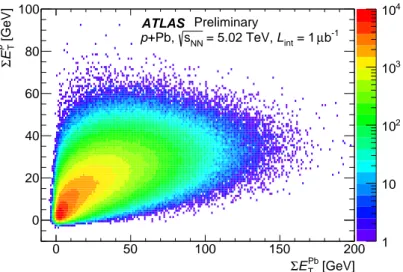
p+Pb collisions included in this analysis,

Fig. 1 shows the correlation between the summed transverse energies measured in the proton-going (−4.9

< η < −3.2) and Pb-going (3.2 < η <

4.9) directions,

ΣE_T^p

and

ΣE^Pb_T

, respectively. The trans- verse energies shown in the figure and used in this analysis were evaluated at the electromagnetic energy scale and have not been corrected for hadronic response. Figure 1 shows that

ΣE^p_T

rapidly saturates with increasing

ΣE^Pb_T

for

ΣE_T^Pb&

30 GeV, indicating that

ΣE_T^p

is less sensitive than

ΣE^Pb_T

to the increased par- ticle production expected to be associated with multiple interactions of the proton in the target nucleus in central collisions. Thus,

ΣE^Pb_T

is used to characterize

p+Pb collision centrality for the analysis presented

here.

The distribution of

ΣE_T^Pb

for events passing the applied

p+

Pb analysis selections is shown in Fig. 2.

Following standard techniques [29], centrality intervals were defined in terms of percentiles of the

ΣE^Pb_T

distribution after accounting for an estimated ine

ffi

ciency (see Appendix A) for inelastic

p+

Pb events to

[GeV]

Pb

ET

Σ

0 50 100 150 200

[GeV]p TEΣ

0 20 40 60 80 100

1 10 102

103

104

ATLAS Preliminary

b-1

µ = 1 Lint

= 5.02 TeV, sNN

+Pb, p

Figure 1: Distribution of proton-going (

ΣE^p_T

) versus Pb-going (

ΣE^Pb_T

) forward calorimeter total trans- verse energy (see text) for

p+Pb collisions included in this analysis.

pass the applied event selections of 1

−ε_inel =

2

±

2%. The following centrality intervals were used in this analysis: 0–1%, 1–5%, 5–10%, 10–20%, 20–30%, 30–40%, 40–60%, 60–90%. The

ΣE^Pb_T

ranges corresponding to these centrality intervals are indicated by the alternating filled and unfilled regions in Fig. 2. The most peripheral 90–100% collisions were excluded from the analysis due to uncertainties

[GeV]

Pb

ET

Σ

0 100 200

]-1 [GeVPb TEΣ/dN devtN1/

10-6

10-5

10-4

10-3

10-2

ATLAS Preliminary

b-1

µ = 1 Lint

= 5.02 TeV, sNN

p+Pb,

Figure 2: Distribution of

ΣE_T^Pb

values for events satisfying all analysis cuts including the Pb-going rapidity gap exclusion (see text). The alternating shaded and unshaded bands indicate centrality intervals, from right to left, 0–1%, 1–5%, 5–10%, 10–20%, 20–30%, 30–40%, 40–60%, 60–90% and 90–100%

(not used in this analysis).

regarding their composition and their reconstruction efficiency.

Following standard procedures, a Glauber analysis [30] was applied to estimate

hN_parti

for each of the centrality intervals used in this analysis. A detailed description of that analysis, which uses the convolution properties of gamma distributions to describe the measured

ΣE^Pb_T

distribution, is provided in Appendix A. Only a summary of the method is given here.

A Glauber Monte Carlo program [44] was used to simulate the geometry of inelastic

p+

Pb collisions

and calculate the probability distribution for

N_part

,

P(Npart

). The simulations used a Woods-Saxon nu- clear density distribution and an inelastic nucleon-nucleon cross-section of

σ_NN=

70

±

5 mb. Separately, PYTHIA8 simulations of

p+p

events were used to obtain a detector-level nucleon-nucleon

ΣE_T^Pb

distri- bution, to be used as input to the Glauber model. This was fit to a gamma distribution. Then, an extension of the wounded-nucleon (WN) model that included non-linear dependence of

ΣE^Pb_T

on

N_part

was used to define

N_part

-dependent gamma distributions for

ΣE_T^Pb

, with the constraint that the distributions reduce to the PYTHIA8 distribution for

N_part =

2. The gamma distributions were summed over

N_part

with a

P(N_part

) weighting to produce a hypothetical

ΣE_T^Pb

distribution. That distribution was fit to the measured

ΣE^Pb_T

distribution shown in Fig. 2 with the parameters of the extended WN model allowed to vary freely.

From the results of the fit, the distribution of

N_part

values and the corresponding

hN_parti, were calculated

for each centrality interval.

In addition to the usual Glauber Monte Carlo simulation, an extension of the Glauber model was also used to calculate

P(Npart

). This takes into account event-to-event fluctuations in the nucleon-nucleon cross-section,

σ_NN

, [31, 32], and is referred to in the rest of this note as “Glauber-Gribov.” Two sets of Glauber-Gribov

N_part

results were obtained for two di

ff

erent values of the parameter,

Ω

, that determines the width of the assumed Gaussian fluctuations in

σ_NN

. For the purposes of this analysis, both values

Ω =

0.55 and

Ω =

1.01 are considered plausible and results from both parameters are studied to evaluate the potential physics implications of the Glauber-Gribov extension.

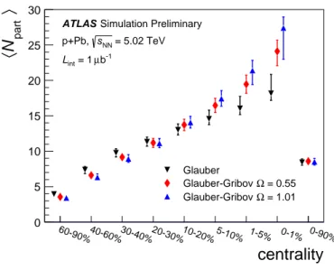
The

hN_parti

values calculated using the above-described procedure are shown in Fig. 3 for the three di

ff

erent

P(N_part

) simulations. The error bars in the figure show asymmetric systematic uncertainties determined by varying di

ff

erent assumptions of the Glauber

/

Glauber-Gribov modeling including

σ_NN

,

ε_inel

, the form of the WN extension, and the properties of the nuclear density distribution. For central collisions, the

hN_parti

uncertainties are dominated by the uncertainty in the WN model extension and

σ_NN

. For more peripheral collisions the uncertainty on

ε_inel

also makes a significant contribution.

The differences in the

hN_parti

values between the Glauber and the two Glauber-Gribov models results from the di

ff

erent shapes of the

p+

Pb

N_part

distributions in these models. The narrower

N_part

distribution in the Glauber model requires larger fluctuations in

ΣE_T^Pb

at fixed

N_part

to describe the tail of the

ΣE^Pb_T

distribution. In contrast, the broader

N_part

distributions associated with the Glauber-Gribov models re- quire smaller intrinsic fluctuations in

ΣE^Pb_T

at fixed

N_part

. As a result, the

hN_parti

corresponding to events with large

ΣE_T^Pb

is systematically larger for the Glauber-Gribov models and is largest for

Ω =

1.01.

6 Measurement of charged particle multiplicity

As described previously, the multiplicity measurement was performed using only the pixel detector to maximize the efficiency for reconstructing charged particles with low transverse momenta. Two ap- proaches are used in this analysis. The first is the two-point tracklet method used widely in heavy ion collision experiments [29, 45, 46]. Two variants of this method have been implemented in this analysis to produce the

dN_ch/dη

result and to estimate the systematic uncertainties, as described below. The second is the use of pixel tracks, described in Section 3. It has a smaller acceptance, but provides measurements of the particle

p_T

. The

dN_ch/dη

measured using pixel tracks is used as a cross-check to that measured using the two-point tracklets.

In the two-point tracklet algorithm, the event vertex and clusters on an inner pixel layer define a

search region for clusters in the outer layers. The algorithm uses all clusters, except for those which

1) have low energy deposits inconsistent with minimum-ionizing particles originating from the primary

vertex, 2) are duplicate clusters resulting from the overlap of the pixel modules or 3) include a small set

of pixels at the centre of the pixel modules that share readout channels [34]. Clusters in the same layer

of the pixel detector were considered as one if they were separated by less than a certain distance. Such

clusters have a high probability to be correlated to the same particle.

centrality

60-90%40-60%30-40%20-30%10-20% 5-10% 1-5% 0-1% 0-90%

〉

part

N 〈

0 5 10 15 20 25 30

Simulation Preliminary ATLAS

= 5.02 TeV sNN

p+Pb, b-1

µ = 1 Lint

Glauber

= 0.55 Ω Glauber-Gribov

= 1.01 Ω Glauber-Gribov

Figure 3:

hN_parti

values resulting from fits to the measured

ΣE^Pb_T

distribution (see Fig. 2) using Glauber and Glauber-Gribov

N_part

distributions. The error bars indicate asymmetric systematic uncertainties (see Appendix A).

The pseudorapidity and azimuthal angle of the cluster in the innermost layer (η, φ) and the difference between those parameters for the cluster in two layers (∆

η,∆φ) are taken as the parameters of the re-

constructed tracklet. The

∆η

of a tracklet is largely determined by the multiple scattering of the incident particles in the material of the beam pipe and detector. This effect plays a less significant role in the

∆φ

of a tracklet, which is driven primarily by the bending of charged particles in the magnetic field, and hence one expects

∆φ

to be larger. The tracklet selection cuts are:

|∆η|<

0.015,

|∆φ|<

0.1,

|∆η|<|∆φ|.

(1)

Keeping tracklets with

|∆φ| <

0.1 corresponds to accepting particles with

p_T &

100 MeV. The depen- dence of the multiple scattering on particle momentum suggests the requirement on the relation between

∆η

and

∆φ

of the tracklet given in the second row of Eq. 1.

The Monte Carlo (MC) simulation for the

dN_ch/dη

analysis is based on the HIJING event generator, which is described in Section 4. Generator (truth) level particles are defined as primary particles if they originate directly from the collision or result from decays of particles with

cτ <

1 mm. All other particles are defined as secondaries. Tracklets are classified as primary or secondary depending on whether the as- sociated truth particle is primary or secondary. Tracklets can also be formed from the random association of hits produced by unrelated particles, or hits in the detector which are not associated to any generated particle. These tracklets are referred to as “fakes”.

The contribution of fake tracklets is relatively di

ffi

cult to model in the simulation, because of the a priori unknown contributions of multiple sources, such as noise clusters or very low energy particles.

To address this problem, the tracklet algorithm is used in two di

ff

erent implementations referred to as

“Method 1” and “Method 2”. In Method 1, at most one tracklet is reconstructed for a given cluster on the first pixel layer. If multiple clusters on the second pixel layer fall within the search region, the resulting tracklets are merged into a single tracklet. This approach limits, but does not eliminate, the presence of fake tracklets. Method 2 reconstructs tracklets for all combinations of clusters in only two pixel layers.

To account for the fake tracklets arising from random combinations of clusters, the same analysis is

performed after inverting the

x

and

y

positions of all clusters on the second layer with respect to the

primary vertex (x

− x_vtx, y−y_vtx

)

→

(−(x

− x_vtx

),

−(y−y_vtx

)). The tracklet yield from this “flipped”

analysis is then subtracted from the original tracklet yield to obtain an estimated yield of true tracklets

N_2p

,

N_2p

(η)

=N_2p^ev

(η)

−N_2p^fl

(η), (2) where

N_2p^ev

represents the yield of two-point tracklets using Method 2 and

N_2p^fl

represents the yield ob- tained by flipping the clusters in the second pixel layer.

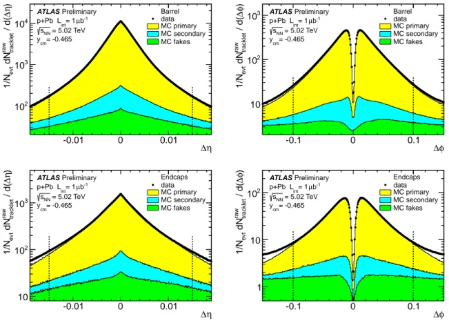
Distributions of

∆η

and

∆φ

of reconstructed tracklets for data and simulated events are shown in Fig. 4 for the barrel (upper) and endcap (lower) parts of the pixel detector. The data is indicated by

η

-0.01 0 0.01 ∆

)η∆ / d(raw tracklet dNevt1/N

102

103

104

Barrel data MC primary MC secondary MC fakes Preliminary

ATLAS b-1

µ

int= 1 p+Pb L

= 5.02 TeV sNN

= -0.465 ycm

φ

-0.1 0 0.1 ∆

)φ∆ / d(raw tracklet dNevt1/N

10 102

103 ^Barrel_data

MC primary MC secondary MC fakes Preliminary

ATLAS b-1

µ

int= 1 p+Pb L

= 5.02 TeV sNN

= -0.465 ycm

η

-0.01 0 0.01 ∆

)η∆ / d(raw tracklet dNevt1/N

10 102

103

Endcaps data MC primary MC secondary MC fakes Preliminary

ATLAS b-1

µ

int= 1 p+Pb L

= 5.02 TeV sNN

= -0.465 ycm

φ

-0.1 0 0.1 ∆

)φ∆ / d(raw tracklet dNevt1/N

1 10 102

Endcaps data MC primary MC secondary MC fakes Preliminary

ATLAS b-1

µ

int= 1 p+Pb L

= 5.02 TeV sNN

= -0.465 ycm

Figure 4:

∆η

(left) and

∆φ

(right) for the tracklets reconstructed with Method 1 measured in the data (circles) and MC (histograms) in

p+Pb collisions at √

sNN =

5.02 TeV. The lowest (green) histogram are the fake tracklets, the middle region (cyan) are secondary particles, and the upper (yellow) region is the contribution of the primary particles.

black circles and simulated events are shown with filled histograms. The simulation results show the three contributions from primary (yellow), secondary (cyan) and fake (green) tracklets. The selection criteria specified by Eq. 1 are shown in Fig. 4 with vertical lines and applied in

∆φ

for

∆η

plots and vice versa. Outside those lines, the contributions of secondary and fake tracklets are more di

ffi

cult to control, especially in the endcap region.

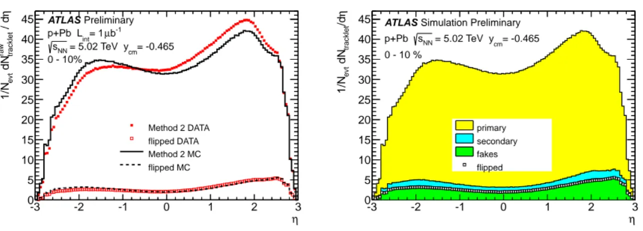
The left panel of Fig. 5 shows the distributions of the number of tracklets reconstructed with Method 2

and satisfying the criteria of Eq. 1 as a function of pseudorapidity in the 0-10% centrality interval for data

(markers) and for the MC (lines). The results of flipped reconstruction are also shown in the plot. Data

and MC distributions are similar but not identical, reflecting the fact that HIJING does not reproduce

-3 -2 -1 0 1 2 η3 η / draw tracklet dNevt1/N

0 5 10 15 20 25 30 35 40

45 ATLAS Preliminary b-1

µ

int= 1 p+Pb L

= -0.465 = 5.02 TeV ycm

sNN

0 - 10%

Method 2 DATA flipped DATA Method 2 MC flipped MC

-3 -2 -1 0 1 2 η3

η/dtracklet dNevt1/N

0 5 10 15 20 25 30 35 40

45 ATLAS Simulation Preliminary

= -0.465 = 5.02 TeV ycm

sNN

p+Pb 0 - 10 %

primary secondary fakes flipped

Figure 5:

η-distribution of number of tracklets reconstructed with Method 2. Left panel shows compar-

ison of the data (markers) to MC (lines). The results of the flipped reconstruction are shown with open markers for data and dashed line for MC. Right panel shows the result of MC for three contributions: pri- mary (yellow) secondary (cyan) and fake (green). Square markers show the result of simulation obtained with flipped reconstruction events.

the data in detail. A breakdown of the MC distribution into primary, secondary and fake contributions is shown in the right panel of Fig. 5. The distribution of

N_2p^fl

(η) given in eq. 2 and plotted with open markers follows exactly the green histogram, which justifies the subtraction of the fake component in Method 2. Of the three methods used in this analysis, Method 2 has the largest contribution of fakes. In the 0-10% centrality interval, the fake contribution amounts to 8% of the yield at mid-rapidity and up to 16% at large pseudorapidity. In the same centrality interval, the contribution of fakes in Method 1 varies from 2% to 10% and from 0.2% to 1.5% in the pixel track method. Method 1 and the pixel track method rely on the MC to correct for the contribution from fakes and all three methods rely on the MC to correct for the contribution of secondary particles.

The data analysis and corresponding corrections were performed in 8 intervals of detector occupancy (O) parametrized using the number of reconstructed clusters in the first pixel layer, and in 7 intervals of

z_vtx

, each 50 mm wide. For each analysis method, a multiplicative correction factor was obtained from the MC simulations. It corrected for several effects: inactive areas in the detector and reconstruction e

ffi

ciency; contributions of residual fakes and secondary particles; and losses due to track or tracklets selection cuts including particles with

p_T

below 100 MeV. The correction factor is evaluated as a function of occupancy

O, event vertexz_vtx

, and pseudorapidity as:

C(O,z_vtx, η)≡ N_pr

(O,

z_vtx, η)

N_rec

(O,

z_vtx, η),

(3) where

N_pr

and

N_rec

represent the number particles at the generator level and the number of tracks or tracklets at the reconstruction level respectively. These factors are then applied to obtain the corrected, per-event charged particle pseudorapidity distributions according to

dN_ch dη =

1

N_evt X

z_vtx

∆N^raw

(O,

z_vtx, η)C(O,z_vtx, η)

∆η ,

(4)

where

∆N^raw

indicates either the number of reconstructed pixel tracks or two-point tracklets and

N_evt

is the total number of analysed events.

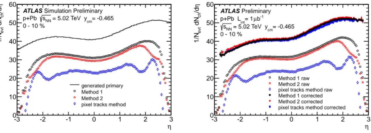
Figure 6 shows the effect of the applied correction for all three methods. The left panel shows the

-3 -2 -1 0 1 2 η3 η/dch dNevt1/N

0 10 20 30 40 50 60

Simulation Preliminary ATLAS

= -0.465 = 5.02 TeV ycm

sNN

p+Pb 0 - 10 %

generated primary Method 1 Method 2 pixel tracks method

-3 -2 -1 0 1 2 η3

η/dch dNevt1/N

0 10 20 30 40 50 60

Preliminary ATLAS

b-1

µ

int= 1 p+Pb L

= -0.465 = 5.02 TeV ycm

sNN

0 - 10 %

Method 1 raw Method 2 raw pixel tracks method raw Method 1 corrected Method 2 corrected pixel tracks method corrected

Figure 6: Left:

η-distribution from the MC for the generated primary charged particles (histogram),

tracklets from Method 1 (circles), tracklets from Method 2 after flipped event subtraction (squares), and pixel tracks (diamonds). Right: Open markers represent the same distributions as in the left panel, reconstructed in the data. Filled markers of the same shape represent corrected distributions.

MC results based on HIJING. The distribution of generated primary charged particles is shown by a solid line and the distributions of reconstructed tracks and tracklets are indicated by markers. Among the three methods, the correction factors for Method 1 are the smallest, while the pixel track method requires the largest corrections. The variation of the reconstructed distribution for the pixel track method around

η = ±2 is related to the transition between the barrel and endcap regions of the detector. The

open markers in the right panel of Fig. 6 show the reconstructed distribution from the data and the filled markers are the corresponding distribution for the three methods after applying corrections. The corrected results are in good agreement with each other, which demonstrates that the rejection of fakes and the rest of the correction procedure are well understood. In this analysis Method 1 is chosen as the default result for

dN_ch/dη, Method 2 is used for systematic uncertainties and the pixel track method is

used primarily as a consistency test, as discussed in detail below.

7 Systematic uncertainties

The systematic uncertainties on

dN_ch/dη

measurement arise from three main sources: 1) inaccuracies of detector description in simulations, 2) sensitivity to selection criteria used in the analysis, including the residual contributions of fakes and secondaries and 3) differences between the generated particles used in the simulation and the data. To extract uncertainties for each source, one of the parameters used in the analysis, such as tracklets selection criteria, simulated particle composition, etc. was altered within acceptable limits. The analysis was performed fully for each variation of the parameters and compared to the standard results of Method 1.

The uncertainty on the detector description arises primarily from the details of the pixel detector acceptance and efficiency. The locations of the inactive pixel modules were precisely matched between the data and simulation. Areas smaller than a single module which were found to have intermittent ine

ffi

ciencies were estimated to contribute less than 1.7% uncertainty to the final result. This uncertainty has no centrality dependence, and is approximately independent of pseudorapidity.

The uncertainties related to the description of the inactive detector material were evaluated using a

MC sample with 10% extra material. The net e

ff

ect on the final result is found to be 2%, independent of

centrality.

Uncertainties due to tracklet selection cuts were evaluated by independently varying the cuts on

|∆η|

and

|∆φ|

up and down by 40%. The e

ff

ect of these variations is less than 1%, except at high-η, and has only a weak centrality dependence.

The HIJING event generator used in the analysis is known to be inconsistent with the

p_T

distributions measured in data. This was addressed by re-weighting the HIJING distribution using the reconstructed spectrum measured with the pixel track method. Since a full spectral analysis was not performed in the framework of this

dN_ch/dη

measurement, the systematic uncertainty on this procedure was assigned to be equal to the magnitude of the variation produced by the re-weighting procedure. This is less than 0.5%

for

|η| <

1.5 and grows to 3.0% towards the edges of the

η

acceptance. The uncertainty has a centrality dependence because the

p_T

distributions in central and peripheral collisions are different.

Tracklets are reconstructed in Method 1 for particles with

p_T >

100 MeV. The unmeasured region of the spectrum contributes approximately 6% to the final

dN_ch/dη. The systematic uncertainty on the ex-

trapolation to

p_T=0 is partially included in the variation of the tracklet∆φ

selection criteria. In addition, this uncertainty was evaluated by varying the shape of the spectra below 100 MeV. This uncertainty was conservatively estimated to reach up to 2.5% at high

η

and has a weak centrality dependence.

To test the sensitivity to the particle composition in HIJING, the fraction of pions, kaons and protons in HIJING were varied within a range according to the di

ff

erences between

p+p

and Pb

+

Pb measured by the CMS and ALICE experiments [47, 48]. The resulting changes of

dN_ch/dη

are found to be less than 1% for all centrality intervals.

The three methods have quite di

ff

erent sensitivities to fake tracks and tracklets. While all three meth- ods agree with each other very well, Method 1 and Method 2 require corrections of a similar magnitude while the pixel track method requires significantly larger correction. The uncertainties due to the pres- ence of residual fakes are estimated by comparing the results between the two tracklet methods. The di

ff

erence in the most central collisions is found to be less than 1.5% in the barrel region and increases to about 2.5% at the far edges of the measured pseudorapidity range.

The uncertainty related to the event selection procedure described in Section 5 is evaluated by varying the

ΣE^Pb_T

ranges used to define centrality intervals, according to an overall trigger and event selection efficiency of 98

±

2%. The variation is performed by generating new centrality intervals assuming this e

ffi

ciency is 96% and 100%. This resulting change of the

dN_ch/dη

is less than 0.5% in central collisions and increase to 6% in peripheral collisions.

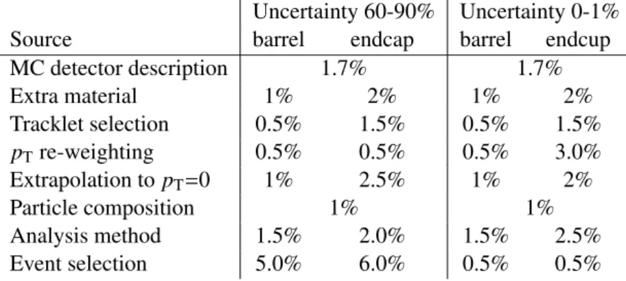
The systematic uncertainties are summarized in Table 1. All uncertainties are treated as independent, so the resulting total systematic uncertainty is a quadratic sum of the individual contributions.

Uncertainty 60-90% Uncertainty 0-1%

Source barrel endcap barrel endcup

MC detector description 1.7% 1.7%

Extra material 1% 2% 1% 2%

Tracklet selection 0.5% 1.5% 0.5% 1.5%

p_T

re-weighting 0.5% 0.5% 0.5% 3.0%

Extrapolation to

p_T=

0 1% 2.5% 1% 2%

Particle composition 1% 1%

Analysis method 1.5% 2.0% 1.5% 2.5%

Event selection 5.0% 6.0% 0.5% 0.5%

Table 1: Summary of the various sources of systematic uncertainties and their estimated impact on the

dN_ch/dη

measurement in central (0-1%) and peripheral (60-90%)

p+

Pb collisions.

8 Results

Figure 7 presents the charged particle pseudorapidity density for

p+

Pb collisions at

√

s_NN =

5.02 TeV in the pseudorapidity interval

|η| <

2.7 for eight centrality intervals. In the most peripheral collisions

-3 -2 -1 0 1 2 η 3

η /d

ch

dN

0 10 20 30 40 50 60

70

ATLAS Preliminary b-1

µ

int= 1 p+Pb L

= 5.02 TeV sNN

= -0.465 ycm

0-1%

1-5%

5-10%

10-20%

20-30%

30-40%

40-60%

60-90%

Figure 7:

dN_ch/dη

measured in different centrality intervals. Statistical uncertainties, shown with vertical bars are typically smaller than the marker size, colour band shows the systematic uncertainty of the results.

(centrality interval 60-90%)

dN_ch/dη

has what appears to be a double-peak structure, similar to that seen in proton-proton collisions [35, 49]. In more central collisions, the shape of

dN_ch/dη

becomes progres- sively more asymmetric, with more particles produced in the Pb-going direction than in the proton-going direction.

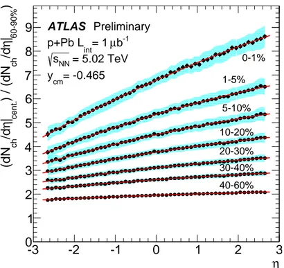
To investigate further the centrality evolution, the distributions in the various centrality intervals are divided by the distribution in the 60-90% centrality interval. The ratios are shown in Fig. 8. The double peak structure seen in the distributions in Fig. 7 disappears in the ratios. The ratios are observed to grow nearly linearly with pseudorapidity, with a slope that increases from peripheral to central collisions. In the 0-1% centrality interval, the ratio increases by almost a factor of two over the measured

η-range. These

ratios are fit with a second-order polynomial function, and the fit results are summarized in Table 2.

Figure 9 shows the

dN_ch/dη

divided by the number of participant pairs (

hN_parti/2) as a function

of

hN_parti

for three different implementations of the Glauber model; standard Glauber (top panel) and Glauber-Gribov model with

Ω =

0.55 and 1.01 in the middle and lower panels respectively. Since the charged particle yields have significant pseudorapidity dependence, the

dN_ch/dη/(hN_parti/2) is presented

in five

η

intervals including the full pseudorapidity interval,

−2.7< η <

2.7.

The

dN_ch/dη/(hN_parti/2) values from the standard Glauber model are approximately constant up to hN_parti ≈

10 and then increase for larger

hN_parti

. This trend is absent in the Glauber-Gribov model with

Ω =

0.55, which shows a relatively constant behaviour for the integrated yield divided by the number of

participant pairs. Finally, the

dN_ch/dη/(hN_parti/2) values from the Glauber-Gribov model withΩ =

1.01

-3 -2 -1 0 1 2 η 3 )

60-90%

| η /d

ch

) / (dN

cent.

| η /d

ch

(dN

0 1 2 3 4 5 6 7 8

9

ATLAS Preliminary b-1

µ

int= 1 p+Pb L

= 5.02 TeV sNN

= -0.465 ycm

0-1%

1-5%

5-10%

10-20%

20-30%

30-40%

40-60%

Figure 8: Ratios of

dN_ch/dη

distributions measured in di

ff

erent centrality intervals,

dN_ch/dη|_cent

, to that in the peripheral (60-90%) centrality interval. Lines show the results of second order polynomial fits to the data points.

Centrality ratio

c b a

0 - 1%

/

60 - 90% 6.78

±

0.28 0.77

±

0.05 -0.033

±

0.006 1 - 5%

/

60 - 90% 5.35±0.22 0.515±0.031 -0.030±0.005 5 - 10%

/

60 - 90% 4.49±0.18 0.377±0.021 -0.0218±0.0035 10 - 20%

/

60 - 90% 3.77

±

0.14 0.269

±

0.014 -0.0169

±

0.0025 20 - 30%

/

60 - 90% 3.11±0.11 0.182±0.010 -0.0113±0.0020 30 - 40%

/

60 - 90% 2.61±0.08 0.122±0.006 -0.0076±0.0016 40 - 60%

/

60 - 90% 1.95

±

0.06 0.0595

±

0.0031 -0.0037

±

0.0011

Table 2: Parameters of second order polynomial fits (c

+bη+aη²

) to

dN_ch/dη

ratios shown in Fig. 8. The stated uncertainties combined statistical and systematic contributions, with the latter making the larger contribution.

show a slight decrease with

hN_parti

in all

η

intervals.

The presence or absence of

hN_parti

scaling does not in itself suggest a preference for one or another of

the implementations of the Glauber model. However, this study emphasizes that considering fluctuations

of the nucleon-nucleon cross section in the Glauber-Gribov model may lead to significant changes in the

N_part

scaling behaviour of the

p+

Pb

dN_ch/dη

data and, thus, their possible interpretations.

0 10 20 30

/2) 〉

part

N 〈 / ( η /d

ch

dN

2 4 6

8

ATLAS Preliminary b-1

µ = 1 p+Pb Lint

= 5.02 TeV sNN

= -0.465 ycm

< 2.7 η -2.7 <

< 2.7 η 2 <

< 1 η 0 <

< 0 η -1 <

< -2 η -2.7 <

Glauber

0 10 20 30

2 4 6 8

=0.55 Ω Glauber-Gribov

〉 N

part

0 10 20 〈 30

2 4 6 8

0

=1.01 Ω Glauber-Gribov

Figure 9:

dN_ch/dη/(hN_parti/2) as a function ofhN_parti

in several

η-regions for the three implementations

of the Glauber model: the standard Glauber model (top panel), the Glauber-Gribov model with

Ω=0.55

(middle panel) and the Glauber-Gribov model with

Ω=1.01 (bottom panel). The open boxes represent

the systematic uncertainty of the

dN_ch/dη

measurement only, and the width of the box is chosen for better visibility (they are not shown for

−

1.0

< η <

0 and 0

< η <

1). The shaded boxes represent the total uncertainty, which is dominated by the uncertainty on the

hN_parti

given in Table 4 and Fig. 3.

They are shown for

−2.7 < η <

2.7. Note that this uncertainty is asymmetric in both directions, due to the asymmetric nature of the uncertainties on

hN_parti. The statistical uncertainties are smaller than the

marker size for all points.

9 Conclusions

This note presents ATLAS measurements of the centrality dependence of the charged particle pseu- dorapidity distribution,

dN_ch/dη, in p+

Pb collisions at a nucleon-nucleon centre-of-mass energy of

√sNN =

5.02 TeV. The results are shown as a function of pseudorapidity over the range

−

2.7

< η <

2.7

and for the 90% most central

p+Pb collisions. The analysis was performed primarily with the ATLAS

pixel detector, and the collision centrality was defined using a forward calorimeter covering 3.2

< η <

4.9

in the Pb-going direction. The average number of participants in each centrality interval,

hN_parti

, was es-

timated using a Monte Carlo Glauber model. The Glauber modeling was performed both in the standard

way, with a fixed nucleon-nucleon cross section, as well as in a Glauber-Gribov approach, which allows

the nucleon-nucleon cross section to fluctuate event-by-event.

The shape of

dN_ch/dη

evolves gradually with centrality from an approximately symmetric shape in the most peripheral collisions to a highly asymmetric distribution in the most central collisions. The ratios of

dN_ch/dη

distributions in different centrality intervals to the

dN_ch/dη

in the most peripheral interval are approximately linear in

η

with a slope that is strongly dependent on centrality.

The

N_part

dependence of

dN_ch/dη/(hN_parti/2) was found to be sensitive to the Glauber modeling,

especially in the most central collisions: while the standard Glauber modeling leads to a strong increase in the multiplicity per participant pair for the 30% most central collisions, the Glauber-Gribov approach leads to a much milder centrality dependence. These results point to the importance of understanding not just the initial state of the nuclear wave function, but also the fluctuating nature of nucleon-nucleon collisions themselves. A deeper understanding of this physics is needed before more precise connections can be made between particle production and the geometry of the initial state.

References

[1] L. P. Csernai, J. Kapusta, and L. D. McLerran, Phys. Rev. Lett.

97

(2006) 152303, arXiv:nucl-th/0604032 [nucl-th].

[2] W. Busza and R. Ledoux, Ann. Rev. Nucl. Part. Sci.

38

(1988) 119–159.

[3] J. Elias, W. Busza, C. Halliwell, D. Luckey, P. Swartz, et al., Phys. Rev. D

22

(1980) 13.

[4] Bari-Cracow-Liverpool-Munich-Nijmegen Collaboration Collaboration, C. De Marzo et al., Phys. Rev. D

26

(1982) 1019.

[5] D. Brick, M. Widgo

ff

, P. Beilliere, P. Lutz, J. Narjoux, et al., Phys. Rev. D

39

(1989) 2484–2493.

[6] PHOBOS Collaboration, B. Back et al., Phys. Rev. Lett.

93

(2004) 082301, arXiv:nucl-ex/0311009 [nucl-ex].

[7] ALICE Collaboration, Phys. Rev. Lett. 110

082302

(2013), arXiv:1210.4520 [nucl-ex].

[8] C. De Marzo, M. De Palma, A. Distante, C. Favuzzi, P. Lavopa, et al., Phys. Rev. D

29

(1984) 2476–2482.

[9] PHOBOS Collaboration, B. Back et al., Phys. Rev.

C72

(2005) 031901, arXiv:nucl-ex/0409021 [nucl-ex].

[10] PHENIX Collaboration, S. Adler et al., Phys. Rev.

C77

(2008) 014905, arXiv:0708.2416 [nucl-ex].

[11] A. Bialas, M. Bleszynski, and W. Czyz, Nucl. Phys.

B111

(1976) 461.

[12] D. H. Brick et al., Phys. Rev. D

41

(1990) 765–773.

[13] A. Adil and M. Gyulassy, Phys.Rev.

C72

(2005) 034907, arXiv:nucl-th/0505004 [nucl-th].

[14] P. Tribedy and R. Venugopalan, Phys. Lett.

B710

(2012) 125–133, arXiv:1112.2445 [hep-ph].

[15] J. L. Albacete, A. Dumitru, and C. Marquet, Int. J. Mod. Phys.

A28

(2013) 1340010,

arXiv:1302.6433 [hep-ph].

[16] ALICE Collaboration, Phys. Rev. Lett.

110

(2013) 032301, arXiv:1210.3615 [nucl-ex].

[17] CMS Collaboration, Phys. Lett.

B718

(2013) 795–814, arXiv:1210.5482 [nucl-ex].

[18] ALICE Collaboration, Phys. Lett.

B719

(2013) 29–41, arXiv:1212.2001.

[19] ATLAS Collaboration, Phys. Rev. Lett.

110

(2013) 182302, arXiv:1212.5198 [hep-ex].

[20] CMS Collaboration, Phys. Lett.

B724

(2013) 213–240, arXiv:1305.0609 [nucl-ex].

[21] ATLAS Collaboration, Phys. Lett.

B725

(2013) 60–78, arXiv:1303.2084 [hep-ex].

[22] K. Dusling and R. Venugopalan, Phys. Rev.

D87

(2013) 054014, arXiv:1211.3701 [hep-ph].

[23] K. Dusling and R. Venugopalan, Phys. Rev.

D87

(2013) 094034, arXiv:1302.7018 [hep-ph].

[24] P. Bozek and W. Broniowski, Phys. Rev.

C88

(2013) 014903, arXiv:1304.3044 [nucl-th].

[25] E. Shuryak and I. Zahed, arXiv:1301.4470 [hep-ph].

[26] A. Bzdak, B. Schenke, P. Tribedy, and R. Venugopalan, arXiv:1304.3403 [nucl-th].

[27] G.-Y. Qin and B. Mller, arXiv:1306.3439 [nucl-th].

[28] W. Broniowski and P. Bozek, arXiv:1308.2370 [nucl-th].

[29] ATLAS Collaboration, Phys. Lett.

B710

(2012) 363–382, arXiv:1108.6027 [hep-ex].

[30] M. L. Miller, K. Reygers, S. J. Sanders, and P. Steinberg, Ann. Rev. Nucl. Part. Sci.

57

(2007) 205–243.

[31] V. Guzey and M. Strikman, Phys. Lett.

B633

(2006) 245–252, arXiv:hep-ph/0505088 [hep-ph].

[32] M. Alvioli and M. Strikman, Phys. Lett.

B722

(2013) 347–354, arXiv:1301.0728 [hep-ph].

[33] ATLAS Collaboration, Eur. Phys. J.

C72

(2012) 1849.

[34] G. Aad, M. Ackers, F. Alberti, M. Aleppo, G. Alimonti, et al., JINST

3

(2008) P07007.

[35] ATLAS Collaboration, New J. Phys.

13

(2011) 053033, arXiv:1012.5104 [hep-ex].

[36] ATLAS Collaboration, Eur. Phys. J.

C72

(2012) 1926, arXiv:1201.2808 [hep-ex].

[37] X.-N. Wang and M. Gyulassy, Phys. Rev.

D44

(1991) 3501–3516.

[38] GEANT4 Collaboration, S. Agostinelli et al., Nucl. Instrum. Meth.

A506

(2003) 250–303.

[39] ATLAS Collaboration, Eur. Phys. J.

C70

(2010) 823–874, arXiv:1005.4568 [physics.ins-det].

[40] T. Sjostrand, S. Mrenna, and P. Z. Skands, JHEP

05

(2006) 026.

[41] ATLAS Collaboration,, “Summary of ATLAS Pythia 8 tunes.”

https://cds.cern.ch/record/1363300. ATL-PHYS-PUB-2011-009.

[42] ATLAS Collaboration,, “ATLAS tunes of PYTHIA 6 and Pythia 8 for MC11.”

https://cds.cern.ch/record/1474107. ATL-PHYS-PUB-2012-003.

[43] ATLAS Collaboration, Phys. Lett.

B707

(2012) 330–348, 1108.6018.

[44] B. Alver, M. Baker, C. Loizides, and P. Steinberg, arXiv:0805.4411.

[45] PHENIX Collaboration, K. Adcox et al., Phys. Rev. Lett.

86

(2001) 3500–3505, nucl-ex/0012008.

[46] PHOBOS Collaboration, B. Alver et al., Phys. Rev.

C83

(2011) 024913, arXiv:1011.1940 [nucl-ex].

[47] CMS Collaboration, arXiv:1307.3442 [hep-ex].

[48] ALICE Collaboration, L. Barnby, AIP Conf.Proc.

1422

(2012) 85–91, arXiv:1110.4240 [nucl-ex].

[49] ATLAS Collaboration, Phys. Lett.

B688

(2010) 21–42, arXiv:1003.3124 [hep-ex].

[50] V. Gribov, Sov. Phys. JETP

29

(1969) 483–487.

[51] H. Heiselberg, G. Baym, B. Blaettel, L. Frankfurt, and M. Strikman, Phys. Rev. Lett.

67

(1991) 2946–2949.

[52] A. Donnachie and P. Landsho

ff

, Phys. Lett.

B296

(1992) 227–232, arXiv:hep-ph/9209205 [hep-ph].

[53] TOTEM Collaboration, G. Antchev et al., Phys. Rev. Lett.

111

(2013) 012001.

[54] H. De Vries, C. De Jager, and C. De Vries, Atom. Data Nucl. Data Tabl.

36

(1987) 495–536.

[55] M. Tannenbaum, Prog. Part. Nucl. Phys.

53

(2004) 239–252.

[56] P. Steinberg, arXiv:nucl-ex/0703002 [NUCL-EX].

[57] ATLAS Collaboration, JHEP

1211

(2012) 033, arXiv:1208.6256 [hep-ex].

Appendix A: Glauber and Glauber-Gribov analysis

The geometry of nucleus-nucleus (A

+

A) and proton

/

deuteron-nucleus (p

/d+

A) collisions is often stud- ied using Glauber Monte Carlo models [30, 44] that simulate the interactions of the incident nucleons using a semi-classical eikonal approximation. However, it has been argued that in high energy

p+A

collisions, the Glauber model must be corrected to account for the fact that the incoming proton is o

ff

shell between successive interactions in the target nucleus[50]. In addition, event-to-event fluctuations in the configuration of the incoming proton can change its effective scattering cross-section [51, 31, 32].

At high energies, the configuration of the proton is taken to be frozen over the time scale of the

p+

A collision. To evaluate the impact of these frozen fluctuations of the projectile proton, a modified ver- sion of the PHOBOS Glauber Monte Carlo [44], referred to as “Glauber-Gribov” in the rest of this note, was developed that implemented event-to-event variations in the Glauber Monte Carlo nucleon-nucleon cross-section. Following Refs. [31] and [32], the probability distribution of

σ_tot

values was taken to be

²

Ph

(σ

_tot

)

=ρ σ_tot σ_tot+σ₀

exp

(

−

(σ

_tot/σ₀−

1)

² Ω²

)

.

(5)

Here,

ρ

is a normalization constant,

Ω

controls the width of the

Ph

(σ

_tot

) distribution, and

σ₀

determines

hσ_toti. The inelastic fraction of the total cross-section is taken to be constant [32],σ_NN = λσ_tot

, so the probability distribution for

σ_NN

is given by

PH

(σ

_NN

)

=

1

λP(σ_NN/λ)

(6)

Estimates of

Ω

were provided in Ref. [31] for centre-of-mass energies 1.8, 9, and 14 TeV. An interpola- tion of those values to

√

s_NN =

5.02 TeV for use in this analysis yielded

Ω =

0.55, a value that is only marginally larger than the value at 9 TeV,

Ω =

0.52. The corresponding value of

σ₀=

78.6 mb was de- termined by requiring a total cross-section,

σ_tot=

86 mb, consistent with the Donnachie and Landshoff [52] parameterization used in [31]. An alternative choice of

σtot

consistent with more recent measure- ments [53] has only a small e

ff

ect on the final distribution. Recently, updated estimates,

Ω =

1.01 and

σ₀ =

72.5 mb corresponding to

σ_tot=

94.8 mb were obtained [32] using results of diffraction measure- ments at the LHC. For the purposes of this note, the Glauber-Gribov analysis was performed using both

Ω =

0.55 and 1.01 in order to evaluate the sensitivity of the physics conclusions to the choice of

Ω

. For each of the

Ω

values,

λ

was chosen to produce a

σ_NN

value of 70 mb with the results

λ=

0.82 and 0.74, respectively, for

Ω =

0.55 and 1.01.

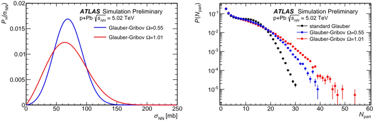
The Glauber-Gribov

P_H

(σ

_NN

) distributions are shown in the left panel of Fig. 10 for both values of

Ω

and corresponding

σ₀

and

λ

values. The distribution of the number of participants,

N_part

, obtained from the two Glauber-Gribov formulations are shown in the right panel of Fig. 10 together with a standard Glauber MC

N_part

distribution obtained using a fixed inelastic cross-section,

σ_NN=

70 mb. For all three calculations, the lead nucleon density distribution was taken to be Woods-Saxon with radius and skin depth parameters,

R=

6.62 fm and

a=

0.546 fm [54]. The Glauber-Gribov

N_part

distributions are much broader than the Glauber distribution due to the

σ_NN

cross-section fluctuations in the Glauber-Gribov formulations.

To connect an experimental measurement of collision centrality such as

ΣE^Pb_T

to the results of the Glauber or Glauber-Gribov Monte Carlo, a model for the

N_part

dependence of the

ΣE_T^Pb

distribution is required. The usual basis for such models, previously applied to A+A and

p/d+A collisions, is the WN

model [11]. When applied to this analysis, this model predicts that

ΣE_T^Pb

would increase proportionally to

N_part

with the proportionality constant equal to one half the corresponding average FCal

^PET

in

p+p

2The first arXiv version of [32] contained a subsequently fixed typographical error that made the distribution exponential instead of Gaussian.