ATLAS-CONF-2014-022 20May2014
ATLAS NOTE
ATLAS-CONF-2014-22
May 18, 2014
Measurement of the correlation between elliptic flow and higher-order flow harmonics in lead–lead collisions at √
s
NN= 2.76 TeV
The ATLAS Collaboration
Abstract
Correlations between the elliptic flow coefficient,
v2, and higher-order flow harmonics,
v3,
v4and
v5are measured using 7
µb−1of Pb+Pb collision data at
√sNN =
2.76 TeV collected by the ATLAS experiment at the LHC. The
v2–v
ncorrelations are measured as a function of centrality, and, for events within the same centrality interval, also as a function of event ellipticity. The results are compared to initial-state eccentricities calculated from initial geometry models. The
v2–v
ncorrelations within a given centrality interval are very di
fferent from the
v2–v
ncorrelations as a function of centrality. For events within the same centrality interval,
v3is found to be anti-correlated with
v2and this anti-correlation is compatible with similar anti-correlations between the corresponding eccentricities
2and
3. On the other hand, the
v4and
v5are found to increase strongly with
v2. The trend and strength of the
v2–v
ncorrelations for
n =4 and 5 are found to disagree with
2–
ncorrelations predicted by initial geometry models. Instead, these correlations are found to be consistent with the combined e
ffects of a linear contribution to
vnand non-linear term that is a function of
v22or of
v2v3, as predicted by hydrodynamic models. A simple two-component fit is used to separate these two contributions. The magnitudes of the linear and non-linear contributions to the
v2–v
4and
v2–v
5correlations are found to be consistent with previously measured event-plane correlations.
c
Copyright 2014 CERN for the benefit of the ATLAS Collaboration.
Reproduction of this article or parts of it is allowed as specified in the CC-BY-3.0 license.
1 Introduction
Heavy ion collisions at the Relativistic Heavy Ion Collider (RHIC) and the Large Hadron Collider (LHC) create hot and dense matter that is thought to be composed of strongly coupled quarks and gluons.
This initially produced matter is lumpy and asymmetric in its shape in the transverse plane [1, 2]. The matter expands under large pressure gradients, which transfer the inhomogenous initial condition into azimuthal anisotropy of produced particles in momentum space [3, 4]. Hydrodynamic models are used to understand the space-time evolution of the matter from the measured azimuthal anisotropy [5–7].
The success of these models in describing the anisotropy of particle production in heavy-ion collisions at RHIC and the LHC [8–14] places important constraints on the transport properties (such as shear viscosity to entropy density ratio) and initial conditions of the produced matter [15–20].
When describing the transverse expansion dynamics, it is convenient to parameterize the final state anisotropy of particle production in terms of a Fourier decomposition in azimuthal angle φ:
dN/dφ∝
1
+2
∞
X
n=1
v
ncos
n(φ−Φn) , (1)
where v
nand
Φnrepresent the magnitude and the phase (referred to as the event plane or EP) of the
nth-order harmonic flow. They are often represented as a two-dimensional vector, or in a complex form:
~v
n=(v
ncos
nΦn, v
nsin
nΦn)
≡v
neinΦn. (2) The presence of harmonic flow has been related to various moments of shape configurations of the initially produced fireball. These moments are described by the eccentricity vector ~
ncalculated from the transverse positions (r, φ) of the participating nucleons relative to their centre of mass [4, 16]:
~
n=(
ncos
nΦ∗n,
nsin
nΦ∗n)
≡neinΦ∗n =−hrneinφihrni
, (3)
where
nand angle
Φ∗n(also known as participant-plane (PP)) represent the magnitude and orientation of the eccentricity vector, respectively. The
h...idenotes an average over the transverse position of all participating nucleons. The eccentricity vectors characterize the spatial anisotropy of the initial produced fireball. According to hydrodynamic model calculations, elliptic flow ~v
2and triangular flow ~v
3are the dominant harmonics, and they are driven mainly by the ellipticity vector ~
2and triangularity vector ~
3of the initially produced fireball [21, 22]:
v
2ei2Φ2 ∝2ei2Φ∗2, v
3ei3Φ3 ∝3ei3Φ∗3. (4) The origin of higher-order (n > 3) harmonics is more complicated; they arise from both ~
nand final state non-linear mixing of lower-order harmonics [20, 22, 23]. For example, an analytical calculation shows that the v
4signal comprises a term proportional to
4(linear response term) and a leading non-linear term that is proportional to
22[22, 24]:
v
4ei4Φ4 = a04ei4Φ∗4 +a1 2ei2Φ∗22+
...
= c0ei4Φ∗4 +c1
v
2ei2Φ22+
... , (5)
where the second line of the equation is derived from Eq. 4, and
c0=a04denotes the linear component
of v
4and coe
fficients
a0,
a1and
c1are weak functions of centrality. The non-linear contribution from v
2is responsible for the strong centrality-dependent event-plane correlation between
Φ2and
Φ4observed
by the ATLAS Collaboration [14]. In the same manner, the v
5signal comprises a linear component proportional to
5and a leading non-linear term involving v
2and v
3[22, 24]:
v
5ei5Φ5 = a05ei5Φ∗5+a12ei2Φ∗23ei3Φ∗3 +...
= c0ei5Φ∗5+c1
v
2v
3ei(2Φ2+3Φ3)+... (6) This decomposition of the v
5signal explains the measured EP correlation involving
Φ2,
Φ3and
Φ5[14].
Another important feature of heavy ion collisions is that the number of participating nucleons is finite and their positions fluctuate randomly in the transverse plane, leading to strong event-by-event (EbyE) fluctuation of
nand
Φ∗n. Calculations based on a Monte-Carlo (MC) Glauber model show that, even for events in a very narrow centrality interval,
ncan fluctuate from zero to several times its mean value, leading to a very broad probability density distribution
p(n) [13]. These fluctuations also re- sult in non-trivial correlations between eccentricities and PP angles of different order characterized by
p(n,
m, ...,
nΦ∗n,
mΦ∗m, ...) [25, 26]. Consequently, such initial geometry fluctuations can influence the development of harmonic flow and lead to non-trivial correlations between final-state flow harmonics characterized by
p(vn, v
m, ...,
nΦn,
mΦm, ...) [20, 21, 26]. Measuring these final-state correlations, and understanding them in terms of both fluctuations of initial-state geometry and final-state non-linear dy- namics is a central focus of current studies of collective flow in heavy ion collisions [7].
ATLAS has recently measured the EbyE distributions of the elliptic and triangular flow,
p(v2) and
p(v3), in lead–lead (Pb+Pb) collisions [13]. This measurement has shown that events within a narrow centrality interval can have very broad
p(v2) and
p(v3) distributions. If events with di
fferent v
2or v
3values could be selected cleanly, one would be able to control the relative contributions of linear and non- linear terms to v
4and v
5in Eqs. 5 and 6, and hence separate these two contributions. An experimental method for selecting on event-shapes has been proposed by several groups [25, 27]. In this method, events in a narrow centrality interval are further classified according to the observed v
msignal (m
=2 and 3) in a forward rapidity range. This classification gives events with similar multiplicity but with very di
fferent ellipticity or triangularity. The values of v
nare then measured at mid-rapidity using the standard flow techniques. Since the
p(vm) distributions are very broad, the correlation between v
mand v
ncan be explored over a wide v
mrange. The event-shape selection technique is sensitive to any differential correlation between
mand
nfor events with the same centrality, which would otherwise be washed-out by averaging over events with di
fferent initial configurations. One example is the strong anti-correlation between
2and
3predicted by the MC Glauber model [25, 28]. A recent transport model calculation shows that this correlation survives the collective expansion and appears as a similar anti-correlation between v
2and v
3[25].
In this note, the correlations between elliptic flow and higher-order flow harmonics are studied using the event-shape selection method. The ellipticity of the events is selected based on the observed v
2signal in a forward pseudorapidity range 3.3 <
|η|< 4.8
1. The values of v
nfor
n =2–5 are then measured at mid-rapidity
|η|< 2.5 using a two-particle correlation method. The extraction of v
nin this analysis is identical to a previous ATLAS publication [11], which is also based on the same dataset. The only di
fference is that, in this analysis, the events are classified both by their centrality as in Ref. [11], as well as the v
2observed at forward pseudorapidity. Most systematics are the shared by the two analyses.
1ATLAS uses a right-handed coordinate system with its origin at the nominal interaction point (IP) in the centre of the detector and thez-axis along the beam pipe. Thex-axis points from the IP to the centre of the LHC ring, and they-axis points upward. Cylindrical coordinates (r, φ) are used in the transverse plane,φbeing the azimuthal angle around the beam pipe. The pseudorapidity is defined in terms of the polar angleθasη=−ln tan(θ/2).
2 ATLAS detector and trigger
The ATLAS detector [29] provides nearly-full solid angle coverage of the collision point with tracking detectors, calorimeters and muon chambers. All of these are well suited for measurements of azimuthal anisotropies over a large pseudorapidity range. This analysis primarily uses two subsystems: the inner detector (ID) and the forward calorimeter (FCal). The ID is contained within the 2 T field of a supercon- ducting solenoid magnet and measures the trajectories of charged particles in the pseudorapidity range
|η|
< 2.5 and over full azimuth. A charged particle passing through the ID traverses typically three mod- ules of the silicon pixel detector (Pixel), four double-sided silicon strip modules of the semiconductor tracker (SCT), and a transition radiation tracker for
|η|< 2. The FCal consists of three longitudinal sampling layers and covers 3.2 <
|η|< 4.9. In heavy ion collisions, the FCal is used mainly to measure the event centrality and event planes [11, 30], though in this analysis it is also used to classify the events in terms of v
2in the forward rapidity region, as described previously.
The minimum-bias Level-1 trigger used for this analysis requires signals in two zero-degree calorime- ters (ZDC) or either of the two minimum-bias trigger scintillator (MBTS) counters. The ZDCs are posi- tioned at 140 m from the collision point, detecting neutrons and photons with
|η|> 8.3, and the MBTS covers 2.1 <
|η|< 3.9 on each side of the nominal interaction point. The ZDC Level-1 trigger thresholds on each side are set below the peak corresponding to a single neutron. A Level-2 timing requirement based on signals from each side of the MBTS is imposed to remove beam backgrounds.
3 Event and track selection
This analysis is based on approximately 7 µb
−1of Pb
+Pb data collected in 2010 at the LHC with a nucleon-nucleon centre-of-mass energy
√sNN =
2.76 TeV. An offline event selection requires a recon- structed vertex and a time difference
|∆t|< 3 ns between the MBTS trigger counters on either side of the interaction point to suppress non-collision backgrounds. A coincidence between the ZDCs at forward and backward pseudorapidity is required to reject a variety of background processes, while maintaining high efficiency for non-Coulomb processes. Events satisfying these conditions are further required to have a reconstructed primary vertex within
|zvtx|< 150 mm of the nominal centre of the ATLAS detector.
The Pb+Pb event centrality [31] is characterized using the total transverse energy (
PET
) deposited in the FCal over the pseudorapidity range 3.2 <
|η|< 4.9 at the electromagnetic energy scale [32].
An analysis of this distribution after all trigger and event selections gives an estimate of the fraction of the sampled non-Coulomb inelastic cross-section to be 98
±2%. The uncertainty associated with the centrality definition is evaluated by varying the effect of trigger and event selection inefficiencies as well as background rejection requirements in the most peripheral FCal
PET
interval [31]. The FCal
P ETdistribution is divided into a set of 5% percentile bins. A centrality interval refers to a percentile range, starting at 0% relative to the most central collisions. Thus the 0–5% centrality interval corresponds to the most central 5% of the events. A MC Glauber analysis [31, 33] is used to estimate the average number of participating nucleons,
Npart, for each centrality interval. These are summarized in Table 1. Following the tradition of heavy ion analysis, the centrality dependence of the results in this note is presented as a function of
Npart.
The harmonic flow coe
fficients, v
n, are measured using tracks reconstructed from hits in the ID for
pT> 0.5 GeV and
|η|< 2.5. At least nine hits in the silicon detectors (out of a typical value of 11) are required for each track, with no missing Pixel hits and not more than one missing SCT hit, taking into account the e
ffects of known dead modules. In addition, the point of closest approach of the track is required to be within 1 mm of the primary vertex in both the transverse and longitudinal directions [30].
The e
fficiency, (
pT, η), of the track reconstruction and track selection cuts is evaluated using Pb
+Pb
Monte Carlo events produced with the HIJING event generator [35]. The generated particles in each
Centrality 0–5% 5–10% 10–15% 15–20% 20–25% 25–30% 30–35%
Npart
382
±2 330
±3 282
±4 240
±4 203
±4 170
±4 142
±4 Centrality 35–40% 40–45% 45–50% 50–55% 55–60% 60–65% 65–70%
Npart
117
±4 95
±4 76
±4 60
±3 46
±3 35
±3 25
±2
Table 1: The list of centrality intervals and associated
Npartvalues used in this analysis. The systematic uncertainties are taken from Ref. [34].
event are rotated in azimuthal angle according to the procedure described in Ref. [36] to give harmonic flow consistent with previous ATLAS measurements [11, 37]. The response of the detector is simulated using GEANT4 [38] and the resulting events are reconstructed with the same algorithms applied to the data. The absolute efficiency increases with
pTby 7% between 0.5 GeV and 0.8 GeV, and varies only weakly for
pT> 0.8 GeV. However, the e
fficiency varies more strongly with η and event multiplicity [39].
For
pT> 0.8 GeV, it ranges from 72% at η
=0 to 57% for
|η|> 2 in peripheral collisions, while it ranges from 72% at η
=0 to about 42% for
|η|> 2 in central collisions.
4 Data Analysis
4.1 Event-shape selection
The ellipticity of the events is characterized with the so-called “flow vector” calculated from the trans- verse energy (E
T) deposited in the FCal [14, 40]:
*q2 =
(q
x,2,
qy,2)
=1
Σ
w
i(Σ[w
icos 2φ
i],
Σ[wisin 2φ
i])
− h*q2ievts(7) (8) where the weight w
iis the
ETof the
ithtower in the FCal. Subtraction of the event-averaged centroid,
h*q2ievts, in Eq. 7 removes biases due to detector effects [41]. The magnitude
q2and the phase
Ψ2of
*q2are calculated for each event as:
q2= q
q2x,2+q2y,2
, tan 2
Ψ2 = qy,2qx,2
. (9)
The angle
Ψ2is the observed event-plane, which is smeared around the true event plane,
Φ2, due to the finite number of particles in an event. A standard technique [42] is used to remove the small residual non- uniformities in the distribution of
Ψ2. These procedures are identical to those used in several previous flow analyses [11, 13, 14, 41]. To reduce the detector nonuniformities at the edge of the FCal, only the FCal towers whose centroids fall within the interval 3.3 <
|η|< 4.8 are used to calculate the flow vector.
The
*q2defined above is insensitive to the energy scale in the calorimeter. In the limit of infinite
multiplicity it approaches the single-particle flow weighted by w:
*q2→(
*v
2)
w = Σw
i(
*v
2)
i/
Σw
i. Hence
the EbyE
q2distribution is expected to follow closely the EbyE v
2distribution, except that it is further
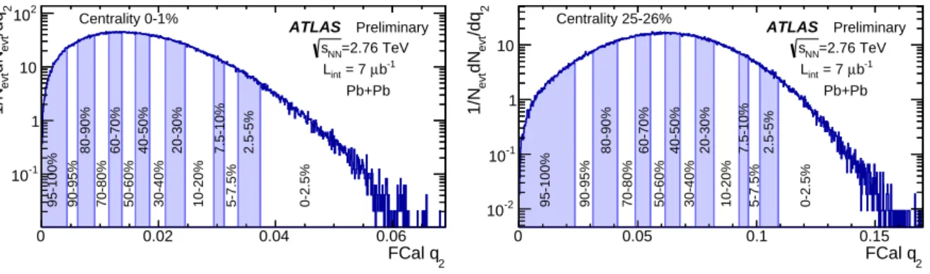
smeared due to the finite number of particles. Figure 1 shows the
q2distributions in two narrow centrality
intervals. These events are first divided into 10 intervals with equal number of events. Since the interval
at the higher (lower) end the distribution covers a much broader
q2range, it is further divided into four
(two) smaller intervals with equal statistics, resulting in a total of fourteen
q2intervals (two 5% intervals,
eight 10% intervals and four 2.5% intervals from low end to high end of the
q2distribution). These
fourteen
q2intervals are defined separately for each 1% centrality interval, and are then grouped together
into the wider centrality intervals used in this analysis (see Table 1). For example, the first
q2interval
for the 0–5% centrality interval is the sum of the first
q2interval in the five centrality intervals, 0–1%,
FCal q2
0 0.02 0.04 0.06
2/dqevtdNevt1/N
10-1
1 10 102
ATLAS Preliminary
=2.76 TeV sNN
b-1
µ = 7 Lint
Pb+Pb Centrality 0-1%
95-100% 90-95% 80-90% 70-80% 60-70% 50-60% 40-50% 30-40% 20-30% 10-20% 7.5-10% 5-7.5% 2.5-5% 0-2.5%
FCal q2
0 0.05 0.1 0.15
2/dqevtdNevt1/N
10-2
10-1
1 10
ATLAS Preliminary
=2.76 TeV sNN
b-1
µ = 7 Lint
Pb+Pb Centrality 25-26%
95-100% 90-95% 80-90% 70-80% 60-70% 50-60% 40-50% 30-40% 20-30% 10-20% 7.5-10% 5-7.5% 2.5-5% 0-2.5%
Figure 1: The distributions of the magnitude of the flow vector,
q2, calculated in the FCal via Eq. 9 in two narrow centrality ranges: 0-1% centrality (left) and 25-26% centrality (right). The vertical lines indicate the boundaries of the fourteen
q2ranges each containing a certain fraction of events as indicated on the plot.
1–2%,..., 4–5%. The default analysis are obtained in the fourteen non-overlapping
q2intervals as defined in Fig. 1. But for better precision, sometimes they are re-grouped into five wider
q2intervals each containing 20% of the statistics, or into two intervals each containing 50% of the statistics.
4.2 Two-particle correlations
The two-particle correlation analysis follows closely a previous ATLAS publication [11] where it is described in detail, so the analysis is only briefly summarized here. For a given event class, the two- particle correlation is measured as a function of relative azimuthal angle
∆φ
=φ
a −φ
band relative pseudorapidity
∆η
=η
a −η
b. The labels a and b denote the two particles in the pair, which may be selected from di
fferent
pTintervals. The two-particle correlation function is constructed as the ratio of distributions for same-event pairs (or foreground pairs
S(
∆φ,
∆η)) and mixed-event pairs (or background pairs
B(∆φ,
∆η)):
C(∆
φ,
∆η)
= S(∆ φ,
∆η)
B(∆
φ,
∆η) . (10)
The mixed-event pair distribution is constructed from track pairs from two separate events with similar centrality and
zvtx, such that it properly accounts for the detector ine
fficiencies and non-uniformity, but contains no physical correlations. In this analysis, charged particles measured by the ID with a pair acceptance extending up to
|∆η|
=5 are used.
This analysis mainly focuses on the shape of the correlation function in
∆φ. A set of 1-D
∆φ correla- tion functions is built from the ratio of the foreground distributions to the background distributions, both projected onto
∆φ.
C(∆
φ)
=R S
(∆ φ,
∆η)d
∆η
R B(∆
φ,
∆η)d
∆η (11) The normalization is fixed by scaling the counts of the mixed-event pairs to be the same as same-event pairs for 2 <
|∆η| < 5, which is then applied for all
∆η slices.
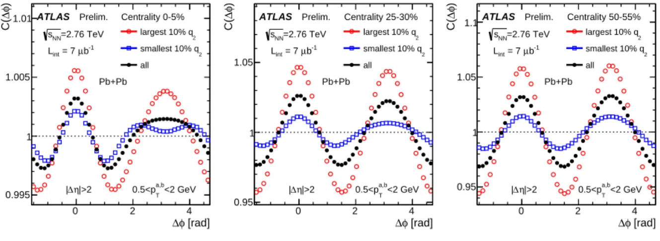
Figure 2 shows the 1-D correlation functions for 2 <
|∆η| < 5 calculated in the low
pTregion
(0.5 <
pa,bT< 2 GeV) in three centrality intervals, 0–5%, 25–30% and 55–60%. For each centrality
interval, the correlation functions are also shown for events selected with largest
q2values and smallest
q2values. The magnitude of the modulation correlates strongly with the
q2value reflecting the fact that
[rad]
φ
0 2 ∆ 4
)φ∆C(
0.995 1 1.005
1.01 ATLAS Prelim.
=2.76 TeV sNN
b-1
µ = 7 Lint
Pb+Pb
Centrality 0-5%
largest 10% q2
smallest 10% q2
all
<2 GeV
a,b
0.5<pT
|>2 η
∆
|
[rad]
φ
0 2 ∆ 4
)φ∆C(
0.95 1 1.05
ATLAS Prelim.
=2.76 TeV sNN
b-1
µ = 7 Lint
Pb+Pb
Centrality 25-30%
largest 10% q2
smallest 10% q2
all
<2 GeV
a,b
0.5<pT
|>2 η
∆
|
[rad]
φ
0 2 ∆ 4
)φ∆C(
0.95 1 1.05
1.1ATLAS Prelim.
=2.76 TeV sNN
b-1
µ = 7 Lint
Pb+Pb
Centrality 50-55%
largest 10% q2
smallest 10% q2
all
<2 GeV
a,b
0.5<pT
|>2 η
∆
|
Figure 2: The correlation functions
C(∆φ) in three centrality intervals for pairs with
|∆η| > 2 and 0.5 <
pT< 2 GeV: 0–5% centrality (left), 25–30% centrality (middle) and 50–55% centrality (right).
For each centrality interval, the correlation functions for events with the largest 10% and smallest 10%
q2
values are also shown. The scale on the y-axis are di
fferent for the three panels. The statistical uncertainties are smaller than the symbols.
the global ellipticity can be controlled by
q2in the forward rapidity. In the 0–5% centrality interval, the correlation function for events with smallest
q2values shows a double-peak structure on the away-side (
∆φ
∼π). This structure reflects the dominant contribution of the v
3when the v
2signal is suppressed by the
q2selection. Similar double-peak strucures are also observed in ultra-central Pb+Pb collisions without event-shape selection [11, 43].
The 1-D correlation function in
∆φ is then expressed as a Fourier series:
C(∆
φ)
=R C(∆
φ)d
∆φ 2π
1
+2
Xn
v
n,n(
paT,
pbT) cos (n
∆φ)
(12)
The coe
fficients are calculated directly from the correlation function as v
n,n = hcos (n∆φ)i. The single- particle azimuthal anisotropy coe
fficients, v
n, are obtained via the factorization relation commonly used for collective flow in heavy ion collisions [11, 12, 44, 45]:
v
n,n(
paT,
pbT)
=v
n(
paT)v
n(p
bT). (13) From this, v
nis calculated as:
v
n(
pT)
=v
n,n(p
T,
prefT)/
qv
n,n(p
refT,
prefT) (14)
where the default transverse momentum range for reference particle,
prefT, is chosen to be 0.5 <
prefT<
2 GeV. The v
nvalues obtained using this method measure, in effect, the root-mean-square (RMS) values of the EbyE v
n[44]. A detailed test of the factorization behaviour has been carried out by comparing the v
n(
pT) obtained for di
fferent
prefTranges in Ref. [11, 12], and factorization holds well for
prefT< 4 GeV.
4.3 Systematic uncertainties
Other than the classification of events according to
q2, the analysis procedure is nearly identical to the
previous ATLAS measurement [11] based on the same dataset. Most systematic uncertainties are the
same, and they are summarized briefly here.
The correlation function relies on the pair acceptance function to reproduce and cancel the detector acceptance e
ffects in the foreground distribution. A natural way of quantifying the influence of detector effects on v
n,nand v
nis to express the single-particle and pair acceptance functions as Fourier series (as in Eq. 12), and measure the coefficients v
detnand v
detn,n. The resulting coefficients for pair acceptance, v
detn,n, are the product of two single-particle acceptances v
det,anand v
det,bn. In general, the pair acceptance function in
∆φ is quite flat: the maximum variation from its average is observed to be less than 0.001, and the corresponding
|vdetn,n|values are found to be less than 1.5
×10
−4. These v
detn,ne
ffects are expected to cancel out to a large extent in the correlation function, and only a small fraction contributes to the uncertainties of the pair acceptance function. Three possible residual e
ffects for v
detn,nare studied in Ref. [11]: 1) the time dependence of the pair acceptance, 2) the e
ffect of imperfect centrality matching, and 3) the e
ffect of imperfect
zvtxmatching. In each case, the residual v
detn,nvalues are evaluated by a Fourier expansion of the ratio of the pair acceptances before and after the variation. The systematic uncertainty of the pair acceptance is the quadrature sum of these three estimates, which is δv
n,n< 5
×10
−6for 2 <
|∆η| < 5.
This absolute uncertainty is propagated to the uncertainty in v
n, and it is the dominant uncertainty when v
nis small, e.g. for v
5in central collisions. This uncertainty has been found to be uncorrelated with the
q2selection, and hence it is assumed not to cancel between di
fferent
q2intervals.
The second type of systematic uncertainty includes the sensitivity of the analysis to track cuts and tracking efficiency, variation of v
nbetween different running periods, and trigger and event selection.
Most systematic uncertainties cancel for the correlation function when dividing the foreground and background distributions. The estimated residual effects are summarized in Table 2. Most of these uncertainties are expected to be correlated between different
q2intervals.
Finally, due to the anisotropy of particle emission, the detector occupancy is expected to be signif- icantly larger in the direction of the event plane where the particle density is larger. This azimuthal angle dependence of the tracking efficiency may lead to a small angle-dependent efficiency variation, which may slightly reduce the measured v
ncoe
fficients. The magnitude of such an occupancy-dependent variation in tracking efficiency has been evaluated using the HIJING simulation with flow imposed on the generated particles [13]. The reconstructed v
nvalues are compared to the generated v
nsignal. The di
fferences are taken as an estimate of the systematics. These di
fferences are found to be 1% or less, and are included in Table 2. Since this effect is proportional to the flow signal, it is expected not to cancel between different
q2ranges.
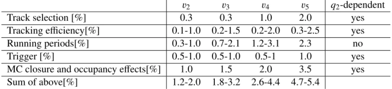
v
2v
3v
4v
5 q2-dependent
Track selection [%] 0.3 0.3 1.0 2.0 yes
Tracking e
fficiency[%] 0.1-1.0 0.2-1.5 0.2-2.0 0.3-2.5 yes
Running periods[%] 0.3-1.0 0.7-2.1 1.2-3.1 2.3 no
Trigger [%] 0.5-1.0 0.5-1.0 0.5-1 1.0 yes
MC closure and occupancy e
ffects[%] 1.0 1.5 2.0 3.5 yes
Sum of above[%] 1.2-2.0 1.8-3.2 2.6-4.4 4.7-5.4
Table 2: Relative systematic uncertainties for v
n, in percent, on the measured v
ndue to tracking cuts,
tracking e
fficiency, variation between di
fferent running periods, centrality variation, consistency between
truth and reconstructed v
nin HIJING simulation, and the quadrature sum of individual terms. Most of
these uncertainties are correlated between different
q2ranges.
2v
0 0.1 0.2 0.3
0-10% of q2
20-30% of q2
all q2
70-80% of q2
90-100% of q2
3v
0 0.05 0.1
ATLAS Preliminary
=2.76 TeV sNN
b-1
µ = 7 Lint
Pb+Pb Centrality 20-30%
<2 GeV
ref
0.5<pT
|>2 η
∆
|
[GeV]
pT
5 10
Ratio
0.5 1 1.5
[GeV]
pT
2 4
Ratio
0.9 1 1.1
4v
0 0.02 0.04 0.06 0.08
ATLAS Preliminary
=2.76 TeV sNN
b-1
µ = 7 Lint
Pb+Pb
5v
0 0.02 0.04
0.06 ATLAS Preliminary
=2.76 TeV sNN
b-1
µ = 7 Lint
Pb+Pb
[GeV]
pT
2 4
Ratio
0.6 0.8 1 1.2
[GeV]
pT
2 4
Ratio
0.6 0.8 1 1.2
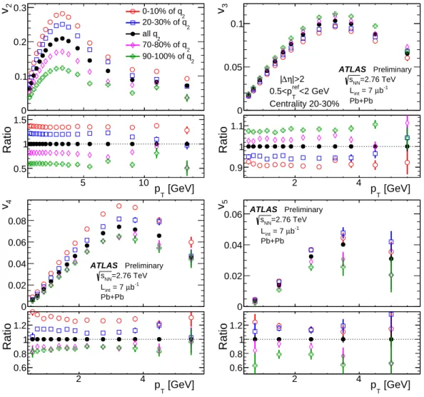
Figure 3: The v
n(
pT) in 20–30% centrality interval for
n=2 (top-left),
n=3 (top-right),
n=4 (bottom- left) and
n =5 (bottom-right). They are calculated for reference
pTof 0.5 <
prefT< 2 GeV. In the top panel of each column, the v
n(p
T) are shown for events in the 0–10%, 20–30%, 70–80% and 90–100% of the
q2ranges (open symbols) as well as for inclusive events without
q2selection (solid symbols). The bottom panel of each column shows the ratios of the v
n(
pT) for
q2-selected events to those obtained for all events. Only statistical uncertainties are shown.
5 Results
5.1 Fourier coe ffi cients, v
n, and their correlations with q
2Figure 3 shows the v
n(
pT) for
n =2–5 extracted from a Fourier decomposition of the one-dimensional (1-D) correlation function in
∆φ, using the relation in Eq. 14, for events in the 20–30% centrality interval.
The results are observed to correlate strongly with the
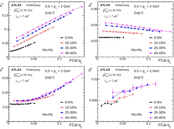
q2selection. The v
2values are largest for events selected with the largest
q2, and smallest for events selected with the smallest
q2, with a total change of more than a factor of two (see ratios in top-left panel). A similar dependence on the
q2selection is also seen for v
4(
pT) and v
5(
pT) (two bottom panels). In contrast to this, the extracted v
3(
pT) values are anti-correlated with the
q2selection; the overall change in v
3(
pT) is also significantly smaller (< 20%
across the
q2range). The relative changes of v
n(p
T) between different
q2ranges are nearly independent
2 FCal q
0 0.05 0.1
2v
0 0.05 0.1 0.15
ATLAS Preliminary
=2.76 TeV sNN
b-1
µ = 7 Lint
< 2 GeV 0.5 < pT
|>2 η
∆
|
Pb+Pb
0-5%
10-15%
25-30%
40-45%
2 FCal q
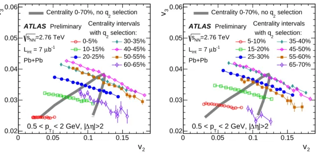
0 0.05 0.1
3v
0 0.02 0.04 0.06
ATLAS Preliminary
=2.76 TeV sNN
b-1
µ = 7 Lint
< 2 GeV 0.5 < pT
|>2 η
∆
|
Pb+Pb
0-5%
10-15%
25-30%
40-45%
2 FCal q
0 0.05 0.1
4v
0 0.01 0.02 0.03
ATLAS Preliminary
=2.76 TeV sNN
b-1
µ = 7 Lint
< 2 GeV 0.5 < pT
|>2 η
∆
|
Pb+Pb
0-5%
10-15%
25-30%
40-45%
2 FCal q
0 0.05 0.1
5v
0 0.005 0.01
ATLAS Preliminary
=2.76 TeV sNN
b-1
µ = 7 Lint
< 2 GeV 0.5 < pT
|>2 η
∆
|
Pb+Pb
0-5%
10-15%
25-30%
40-45%
Figure 4: The correlations between v
nand
q2in four centrality intervals with
n =2–5, where v
nis calculated in 0.5 <
pT< 2 GeV. Each panel shows results for one harmonic. Only statistical uncertainties are shown.
of
pTfor
n=2 and 3, with a possible weak dependence for
n=4 and 5.
Figure 4 shows the correlation between v
nat low
pT(0.5 <
pT< 2 GeV) and
q2for several centrality intervals. Since the relative change of v
nto the
q2selection has a weak
pTdependence, this plot captures the essential features of the correlation between v
nand
q2selection shown in Fig. 3. Due to the finite number of particles in a event, the measured
q2value fluctuates relative to the true value producing a weakening of the
q2–v
ncorrelations. However, for each
q2interval, the elliptic flow can be measured at mid-rapidity and the mapping between FCal
q2and mean v
2can be used to correct the measured
q2–v
ncorrelations in Fig. 4 to proper v
2–v
ncorrelations. Studying the direct correlation between v
2in two different
pTranges, and the correlation between v
2and higher-order flow harmonics are the main subject of this analysis. These correlations provide insights on fluctuations in the collision geometry in the initial state, as well as non-linear dynamics in the final-state collective expansion [21, 22, 25]. Results from these correlations are discussed in detail in the following sections.
5.2 Correlation between the high-p
Tv
2and the low- p
Tv
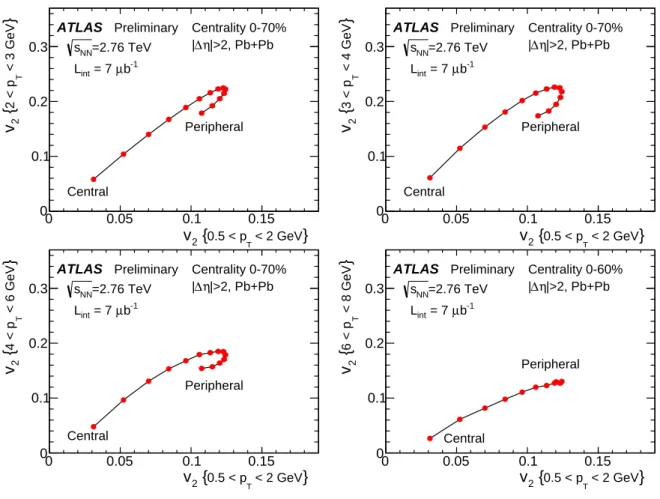
2Figure 5 shows the correlation of v
2between two
pTranges for various centrality intervals. The
x-axis represents v
2values in 0.5–2 GeV range, while the y-axis represents v
2values from a higher
pTrange. Each data point corresponds to a 5% centrality interval within the overall centrality range of 0–
70%. Going from central collisions (left end of the data points) to the peripheral collisions (right end
of the data points), the v
2first increases and then decreases along both axes, reflecting the characteristic
centrality dependence of v
2, well known from pervious flow analyses [10,11]. The rate of decrease of v
2is
}
< 2 GeV 0.5 < pT
2 { v
0 0.05 0.1 0.15
} < 3 GeV T2 < p {2v
0 0.1 0.2 0.3
ATLAS Preliminary
=2.76 TeV sNN
b-1
µ = 7 Lint
|>2, Pb+Pb η
∆
|
Centrality 0-70%
Central
Peripheral
}
< 2 GeV 0.5 < pT
2 { v
0 0.05 0.1 0.15
} < 4 GeV T3 < p { 2v
0 0.1 0.2 0.3
ATLAS Preliminary
=2.76 TeV sNN
b-1
µ = 7 Lint
|>2, Pb+Pb η
∆
|
Centrality 0-70%
Central
Peripheral
}
< 2 GeV 0.5 < pT
2 { v
0 0.05 0.1 0.15
} < 6 GeV T4 < p {2v
0 0.1 0.2 0.3
ATLAS Preliminary
=2.76 TeV sNN
b-1
µ = 7 Lint
|>2, Pb+Pb η
∆
|
Centrality 0-70%
Central
Peripheral
}
< 2 GeV 0.5 < pT
2 { v
0 0.05 0.1 0.15
} < 8 GeV T6 < p { 2v
0 0.1 0.2 0.3
ATLAS Preliminary
=2.76 TeV sNN
b-1
µ = 7 Lint
|>2, Pb+Pb η
∆
|
Centrality 0-60%
Central
Peripheral
Figure 5: The correlation of the v
2in 0.5 <
pT< 2 GeV (x-axis) with v
2in four higher
pTranges (y-axis), one for each panel. In each panel, the v
2values are calculated in fourteen 5% centrality intervals in the centrality range 0–70% without
q2selection, and the data-points for the most central and most peripheral centrality intervals are indicated explicitly. The error bars and shaded boxes represents the statistical and systematic uncertainties, respectively. These uncertainties are often smaller than the symbol size.
larger at intermediate
pT(2 <
pT< 8 GeV), resulting in the boomerang-like structure in the correlation.
The stronger centrality dependence of v
2at higher
pTis consistent with larger viscous-damping effects expected from hydrodynamic calculations [46].
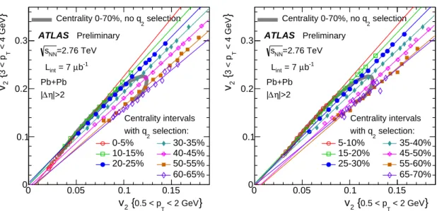
The events in each centrality interval are then further sub-divided into
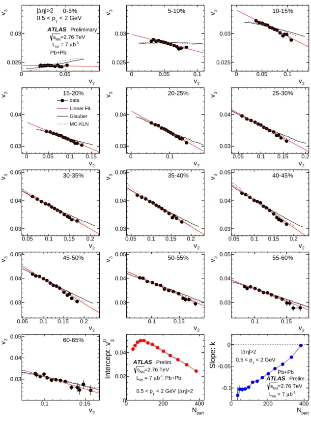
q2intervals, as described above. With this further sub-division each data point in Fig. 5 turns into a group of data points, which may follow a different correlation pattern. Figure 6 shows the v
2correlation between 0.5–2 GeV and 3–
4 GeV for di
fferent
q2event classes (results for other
pTranges are similar). For clarity, the results for the
fourteen different centrality intervals are divided into two different panels, but in each panel the overall
centrality dependence prior to the
q2selection from Fig. 5 (the “boomerang”) is also shown. Unlike
the centrality dependence, the v
2correlation within a given centrality interval follows approximately a
straight line pointing back very close to the origin. This linear relation is quantified by fitting the data to
a linear function in each centrality interval, and the resulting slopes and intercepts are shown in the two
panels of Fig. 7, together with similar results for other
pTranges. The small non-zero intercepts can be
attributed to a residual centrality dependence of the v
2correlation, due to the finite centrality interval used
for each
q2-dependence. This approximately linear correlation suggests that, once the event centrality
or the overall event multiplicity is fixed, the viscous-damping e
ffects on v
2changes very little with the
}
< 2 GeV
T
0.5 < p
2 { v
0 0.05 0.1 0.15
} < 4 GeV T3 < p {2v
0 0.1 0.2
0.3 ATLAS Preliminary
=2.76 TeV sNN
b-1
µ = 7 Lint
Pb+Pb
|>2 η
∆
|
selection Centrality 0-70%, no q2
Centrality intervals selection:
with q2
0-5%
10-15%
20-25%
30-35%
40-45%
50-55%
60-65%
}
< 2 GeV
T
0.5 < p
2 { v
0 0.05 0.1 0.15
} < 4 GeV T3 < p {2v
0 0.1 0.2
0.3 ATLAS Preliminary
=2.76 TeV sNN
b-1
µ = 7 Lint
Pb+Pb
|>2 η
∆
|
selection Centrality 0-70%, no q2
Centrality intervals selection:
with q2
5-10%
15-20%
25-30%
35-40%
45-50%
55-60%
65-70%
Figure 6: The correlation of the v
2in 0.5–2 GeV (x-axis) with v
2in 3–4 GeV range (y-axis) in various centrality intervals. The centrality intervals are staggered into the two panels for clarity. The data points in each centrality interval correspond to the fourteen default
q2intervals. The data are overlaid with the centrality dependence without
q2selection as shown in top-right panel of Fig. 5. The thin solid straight lines represent a linear fit of the data in each centrality, and error bars represent the statistical uncertainties.
Npart
0 100 200 300 400
Slope: K
1 1.5 2 2.5
3 ATLAS Preliminary
=2.76 TeV sNN
b-1
µ = 7 Lint
Pb+Pb < 2 GeV
a
0.5 < pT
<3 GeV
b
2 < pT
<4 GeV
b
3 < pT
<6 GeV
b
4 < pT
Npart
0 100 200 300 400
0Intercept: Y
-0.05 0
0.05 |∆η|>2 ATLAS Preliminary
=2.76 TeV sNN
b-1
µ = 7 Lint
Pb+Pb
+ Y0 a} {pT
= K v2 b} {pT
Fit func.: v2
Figure 7: The slope and intercept of the linear fit of the v
2{pbT}–v2{paT}correlations between low-p
aTrange 0.5 <
paT< 2 GeV and four higher
pbTranges (see text). Only statistical uncertainties are shown.
Examples of the fits are shown in Fig. 6.
variation of the event ellipticity via
q2selection. The influence of viscous corrections on v
2is mainly
controlled by the event centrality (or the overall system size).
2 v
0 0.05 0.1 0.15
3v
0 0.02 0.04
ATLAS Preliminary
=2.76 TeV sNN
b-1
µ = 7
Lint |∆η|>2, Pb+Pb < 2 GeV 0.5 < pT
Centrality 0-70%
Central Peripheral
2 v
0 0.1 0.2 0.3
3v
0 0.05 0.1
ATLAS Preliminary
=2.76 TeV sNN
b-1
µ = 7
Lint |∆η|>2, Pb+Pb < 3 GeV 2 < pT
Centrality 0-70%
Central
Peripheral
2 v
0 0.1 0.2 0.3
3v
0 0.05 0.1
ATLAS Preliminary
=2.76 TeV sNN
b-1
µ = 7
Lint |∆η|>2, Pb+Pb < 4 GeV 3 < pT
Centrality 0-70%
Central
Peripheral
2 v
0 0.1 0.2 0.3
3v
0 0.05 0.1
ATLAS Preliminary
=2.76 TeV sNN
b-1
µ = 7
Lint |∆η|>2, Pb+Pb < 6 GeV 4 < pT
Centrality 0-70%
Central
Peripheral