ATLAS-CONF-2014-026 20May2014
ATLAS NOTE
ATLAS-CONF-2014-026
May 20, 2014
Centrality, rapidity and p
Tdependence of isolated prompt photon production in lead-lead collisions at √
s
NN= 2.76 TeV with the ATLAS detector at the LHC
The ATLAS Collaboration
Abstract
The ATLAS experiment at the LHC has measured prompt photon production in
√sNN=
2.76 TeV Pb+Pb collisions using data collected in 2011 with an integrated luminos-
ity of 0.14 nb
−1. The measurement is performed with a hermetic, longitudinally segmented calorimeter, which gives excellent spatial and energy resolution, and detailed information about the shower shape of each measured photon. A multiparameter selection on a set of nine shower properties, coupled with an isolation criterion based on the energy deposited in the cone around a photon, gives measured purities ranging from 50% at low
pTto greater than 90% at high
pT. Photon yields, scaled by the mean nuclear thickness function, are presented as a function of collision centrality, pseudorapidity (in two intervals
|η| <1.37 and 1.52
< |η| <2.37) and transverse momentum (from 22
< pT <280 GeV). The scaled yields are compared to expectations from JETPHOX (perturbative QCD calculations at next to leading order), as are the ratios of the forward yields to those near mid-rapidity. The ob- served photon yields agree well with the predictions for proton-proton within statistical and systematic uncertainties. Both the yields and ratios are also compared to two other pQCD calculations, one which uses the isospin content appropriate to colliding lead nuclei, and another which includes the EPS09 nuclear modifications to the proton parton distribution functions.
c
Copyright 2014 CERN for the benefit of the ATLAS Collaboration.
Reproduction of this article or parts of it is allowed as specified in the CC-BY-3.0 license.
1 Introduction
Photons are an important tool for the study of the hot, dense matter formed in the high energy collision of heavy ions. Being colorless, they are transparent to the subsequent evolution of the matter and thus probe the very initial state of the collision. Thus, they are expected to be directly sensitive to the overall thickness of the colliding nuclear matter, since their production rates should scale linearly with the num- ber of binary collisions among the nucleons in the oncoming nuclei. Their production is also sensitive to modifications of the partonic structure of nucleons embedded in a nucleus, which are implemented as nuclear modifications [1, 2, 3] to the parton distribution functions (PDFs) measured in deep inelastic and proton-proton scattering experiments (typically called “nPDFs”). Photon rates are also sensitive to the interaction of jets with the medium, via the conversion of jets into photons by re-scattering from quarks and gluons in a hot quark-gluon plasma. This is expected to lead to increased photon production relative to expectations [4].
In general, prompt photons are those that do not arise from hadron decays. Prompt photons have two primary sources. The first is direct emission, which proceeds via quark-gluon Compton scattering
qg → qγor quark-antiquark annihilation
qq →gγ, and higher order extensions. The second is the
“fragmentation” contribution, from the production of a single hard photon during parton fragmentation.
At leading order in QCD perturbation theory, there is a meaningful distinction between the direct emis- sion and fragmentation, but at higher orders the two cannot be unambiguously separated. In order to suppress multi-jet background events from di-jet processes, as well as fragmentation photons, an “iso- lation” criterion is typically applied to energy within a cone of a well-defined radius in η
−φ relative to the photon direction [5]. The isolation transverse energy requirement can be applied as a fraction of the photon transverse energy, or as a constant transverse energy threshold. In either case, these can be applied consistently to perturbative Quantum Chromodynamics (pQCD) calculations so that prompt photon rates can be calculated reliably.
Prompt photon rates have been measured extensively in proton-proton (pp) collisions at the CERN ISR (pp at
√s =
24
−62.4 GeV) [6, 7], and RHIC at Brookhaven (pp at
√s =
200 GeV) [8], and in proton-antiproton collisions at the CERN SppS ( ¯
ppat
√s =
200
−900 GeV) [9] and at the Fermi- lab Tevatron ( ¯
ppfrom
√s =
1.8
−1.96 TeV) [10, 11]. At the LHC, ATLAS [12, 13] and CMS [14]
have measured isolated prompt photons in
ppcollisions at
√s =7 TeV. In all cases, good agreement
has been found with perturbative QCD calculations at NLO, which are typically calculated using the JETPHOX 1.3 package [5, 15]. In lower-energy heavy ion collisions, WA98 observed direct photons in Pb+Pb collisions at
√sNN =
17.3 GeV [16] Pb+Pb collisions, and the PHENIX experiment performed measurements of direct photon rates in gold-gold collisions at
√sNN =
200 GeV [17].
The variable typically used to characterize the modification of hard processes rates in a nuclear environment is the nuclear modification factor
RAA =
(N
X/N
evt)
TAA
σ
ppX, (1)
where
NXis the produced number of objects X,
Nevtis the number of minimum bias events,
TAAis the mean nuclear thickness function (defined as the number of binary collisions divided by the total inelastic nucleon-nucleon (NN) cross section) and σ
ppXis the cross section of process
Xin
ppcollisions.
The use of this formula allows for the straightforward comparison of yields in heavy ion collisions, normalized by the flux of incoming partons, to those measured in
ppdata and calculated using standard calculations. CMS performed the first measurement of isolated prompt photon rates in
ppas well as lead- lead collisions, at nucleon-nucleon center-of-mass energy of
√s =
2.76 TeV [18]. This measurement
found rates consistent with scaling with the number of binary collisions, and thus found
RAAvalues
consistent with unity for all collision impact parameters and
pTranges considered.
This note presents isolated prompt photon yields measured in lead-lead (Pb+Pb) collisions with the ATLAS detector, making use of its large-acceptance, longitudinally segmented calorimeter system.
The underlying event (UE) is found to distort the energy of the measured photon, modify its spatial distribution, and to shift the energy emitted into a cone around the photon, requiring its subtraction in each event. Photon yields are measured over two regions in the pseudorapidity of the photon,
|η|<
1.37 (central) and 1.52 <
|η|< 2.37 (forward), and for 22 <
pT< 280 GeV. A double side-band approach is used to estimate the background from jets in the collision data. Comparisons of the yields with perturbative QCD calculations at next-to-leading order (NLO) are also presented, using JETPHOX 1.3 [15], run in three configurations:
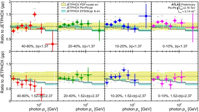
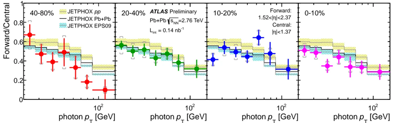
ppcollisions, Pb+Pb collisions (i.e. with the correct total isospin), and Pb+Pb after incorporating the EPS09 nuclear modification factors to the nucleon PDFs. The ratio of the yields in the forward η bin to that in the central η bin,
RFCηη, are also presented, as this quantity is sensitive to nPDF effects, and is less sensitive to some systematic effects.
2 Experimental setup
The ATLAS detector is described in detail in Ref. [19]. It is comprised of three major subsystems, the inner detector, the calorimeter system, and the muon spectrometer.
The ATLAS inner detector is comprised of three major subsystems: the pixel detector, the semicon- ductor tracker (SCT) and the transition radiation tracker (TRT), which cover full azimuth and pseudora- pidity
1over
|η|< 2.5, except for the TRT, which covers
|η|< 2. The muon spectrometer measures muons over
|η|< 2.7 with a combination of monitored drift tubes and cathode strip chambers.
The ATLAS calorimeter is the primary subsystem used for the measurement presented here. It is a large-acceptance, longitudinally-segmented sampling calorimeter covering
|η|< 4.9 with electromag- netic (EM) and hadronic sections. The EM section is a lead-liquid argon sampling calorimeter with an accordion geometry. It is divided into the barrel region, covering
|η|< 1.475, and two endcap re- gions, covering 1.375 <
|η|< 3.2. The EM calorimeter has three primary longitudinal sections, called
“layers”, and is expected to fully contain typical showers. The first sampling layer is 3 to 5 radiation lengths deep and is segmented into fine strips of size
∆η
=0.003
−0.006 (depending on η), which allows the discrimination of photons from the two-photon decays of π
0and η mesons. The second layer is 17 radiation lengths thick, sampling the majority of an electromagnetic shower, and has cells of size
∆η
×∆φ
=0.025
×0.025. The third layer has a material depth ranging from 4 to 15 radiation lengths and is used to catch the tails of high energy electromagnetic showers. In test beam environments and in typical
ppcollisions, the calorimeter energy resolution is found to have a sampling term of 10- 17%/
√E/(1GeV). The total material in front of the electromagnetic calorimeter ranges from 2.5 to 6
radiation lengths depending on pseudorapidity, except in the the transition region between the barrel and endcap regions (1.37 <
|η|< 1.52), in which the material is up to 11.5 radiation lengths. In front of the strip layer, a presampler is used to correct for energy loss in front of the calorimeter within the region
|η|
< 1.8.
The hadronic calorimeter section is located radially outside the electromagnetic calorimeter. Within
|η|
< 1.7, it is a sampling calorimeter of steel and scintillator tiles, with a depth of 7.4 hadronic interaction lengths. In the endcap region it is copper and liquid argon with a depth of 9 interaction lengths.
The ATLAS minimum bias trigger scintillators (MBTS), zero degree calorimeters (ZDCs), and for- ward calorimeter (FCal) are used for minimum-bias event triggering and for determining the “centrality”
of the collision, which can be related to geometric parameters such as the number of participating nu-
1ATLAS uses a right-handed coordinate system with its origin at the nominal interaction point (IP) in the centre of the detector and thez-axis along the beam pipe. Thex-axis points from the IP to the centre of the LHC ring, and theyaxis points upward. Cylindrical coordinates (r, φ) are used in the transverse plane,φbeing the azimuthal angle around the beam pipe. The pseudorapidity is defined in terms of the polar angleθasη=−ln tan(θ/2).
cleons or the number of binary collisions [20]. The MBTS detect charged particles over 2.1 <
|η|< 3.9 using two sets of 16 counters positioned at
z = ±3.6 m. The ZDC detects forward-going neutral par-ticles with
|η|> 8.3. The FCal has three layers in the longitudinal direction, one electromagnetic and two hadronic, covering 3.1 <
|η|< 4.9. The FCal electromagnetic and hadronic modules are composed of copper and tungsten absorbers, respectively, with liquid argon as the active medium, which together provide 10 interaction lengths of material.
The sample of events used in this analysis was collected using the first level calorimeter trigger [21].
This is a hardware trigger which sums the electromagnetic energy in towers of size
∆η
×∆φ
=0.1
×0.1.
A sliding window of size 0.2
×0.2 was used to find electromagnetic clusters by searching for local energy maxima and, keeping only those clusters with energy in two adjacent cells (i.e. regions with a size of either 0.2
×0.1 or 0.1
×0.2) exceeding a threshold. The trigger used for the present measurement had a threshold of 16 GeV, and the trigger performance is described below.
3 Simulated data samples
For the extraction of photon performance parameters (e
fficiencies, photon energy scale, isolation trans- verse energy distributions) two sets of photon+jet events were produced using the ATLAS MC11 [22]
tune of PYTHIA 6.4 [23] at
√s=
2.76 TeV. A set of 4 million photon
+jet events was produced, divided into four sub-samples based on requiring a minimum transverse momentum for the primary photon:
pT
> 17 GeV,
pT> 35 GeV,
pT> 70 GeV,
pT> 140 GeV. Separately, the fragmentation photon con- tribution was modeled using a set of 3 million di-jet events, each with a hard photon produced in the fragmentation of jets produced with the PYTHIA hardness scale, which controls the typical
pTof the produced jets, ranging over
pT =17
−580 GeV. Since a hard photon is only rarely produced in di-jet events, a much larger number of di-jet events needed to be generated in order to produce the simulated sample of fragmentation photons. For both generated samples, each event was fully simulated using GEANT4 [24, 25] with the event vertex of the simulated event matched with the reconstructed vertex of a real minimum-bias event. The simulation output was then digitized and overlaid onto the measured signals the real event. The combined signals were reconstructed and analyzed in the same way as exper- imental data. By using real minimum-bias data as the underlying event model, essentially all features of the data are preserved in the simulation, including the full details of its azimuthal correlations.
Reconstructed photons are considered “matched” to primary truth photons when they are within an angular distance
R= p∆
φ
2+ ∆η
2< 0.2 relative to each other.
4 Collision data selection
The data sample analyzed in this note corresponds to
√ Lint =0.14 nb
−1of Pb+Pb collisions at
sNN=2.76 TeV, collected during the 2011 LHC heavy ion run. After the trigger requirement, events were then further analyzed if they satisfied a set of quality cuts. The relative time measured between the two MBTS counters was required to be less than 5 ns. Both ZDCs were required to give a total energy signal above a threshold set below the measured single neutron peak. Finally, to reject non-collision backgrounds, a vertex is required to be reconstructed in the inner detector.
The centrality of each heavy ion collision is determined using the total transverse energy measured in
the forward calorimeter (3.2 <
|η|< 4.9), at the electromagnetic scale, FCal
ΣET. The trigger and event
selection were studied in detail in the 2010 data sample [26] and 98±2% of the total inelastic cross section
was accepted. The higher luminosity of the 2011 heavy ion run necessitated a more sophisticated trigger
strategy, including more restrictive triggers in the most peripheral events. However, it was found that
the FCal
ΣETdistributions in the 2011 data match those measured in 2010 to a high degree of precision,
[TeV]
ET
Σ FCal
0 1 2 3
[1/TeV]TEΣ/d evt) dN evt(1/N
10-8
10-6
10-4
10-2
1 102
40-80% 20-40% 10-20% 0-10%
Preliminary ATLAS
=2.76 TeV sNN
Pb+Pb Minimum bias 16 GeV EM trigger 40 GeV tight photons
=0.14 nb-1 γ
, Lint
b-1
µ
MB=5 Lint
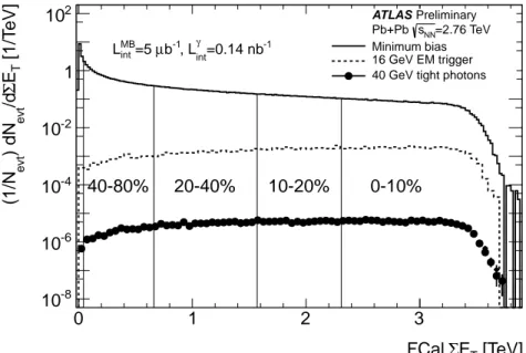
Figure 1: Distribution of FCal
ΣET, at the 2011 energy scale, with centrality bins indicated. The dotted line shows the distribution for minimum bias data, the dashed line shows the distribution of events that trigger the 16 GeV level 1 trigger, and the solid line shows the distribution for photon candidates with
ET> 40 GeV satisfying tight photon selections in the two pseudorapidity regions used for the analysis.
(see section 5).
after accounting for a 4.1% change in the energy calibrations. For this analysis, the FCal
ΣETdistribution (shown in Fig. 1) has been divided into 4 centrality intervals, covering the 0-10%, 10-20%, 20-40% and 40-80% most central events. With this convention, the 0-10% interval has the highest multiplicities, and the 40-80% interval the lowest. These intervals are illustrated by the vertical lines in Fig. 1. The number of sampled minimum bias events corresponding to the 0-80% central interval is
Nevt =763
×10
6.
The FCal
ΣETdistribution is shown in Fig. 1 for three types of events. The top distribution (dotted line) is for the recorded minimum bias events. The dashed line shows the distribution for events that satisfy the L1 trigger. These events are more likely to the more central events, as might be expected if the rates are proportional to the number of binary collisions. Finally, the solid line shows the distributions for photon candidates with
ET> 40 GeV and which satisfy the tight photon selection criteria explained in Section 5. Despite the huge di
fferent in rates, the tight photon candidate distribution is quite similar to the one just triggered by the calorimeter trigger.
The geometric quantities are calculated as described in Ref. [27] using a Glauber Monte Carlo cal-
culation, with a simple implementation of the ATLAS FCal response. Table 1 summarizes all of the
centrality-related information used in this analysis. For each centrality interval, it specifies the FCal
ΣETranges, the mean number of “participants” (nucleons which interact at least once) with its total system-
atic uncertainty, the mean number of binary collisions with its total uncertainty, and finally the mean
value of the nuclear thickness function
hTAAi. The uncertainty on the mean nuclear thickness function TAA = Ncoll/σ
NNis smaller than the corresponding uncertainty on
Ncoll, since the uncertainty on σ
NNlargely cancels in the ratio. The
Ncolluncertainties themselves account for variations in the Glauber
model parameters consistent with the uncertainties in the knowledge of the lead wave function, as well
as uncertainty in the sampled fraction of the inelastic cross section.
Interval
ΣETrange
hNparti δhNpartihNparti hNcolli δhNcolli
hNcolli hTAAi δhTAAi
hTAAi
0-10% 2.31-4 TeV 356 0.7% 1500 8% 23.4 3.0%
10-20% 1.57-2.31 TeV 261 1.4% 923 7% 15.1 3.1%
20-40% 0.66-1.57 TeV 158 2.5% 441 7% 6.88 5.2%
40-80% 0.044-0.66 TeV 45.9 6% 77.8 9% 1.22 9.4%
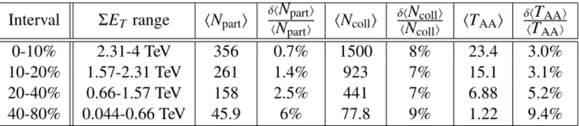
Table 1: Centrality bins used in this analysis, tabulating the percentage range, the FCal
ΣETrange (in 2011), the average number of participants (hN
parti) and binary collisions (hNcolli) and the relativesystematic uncertainty on these quantities.
5 Photon reconstruction
The electromagnetic shower associated with each photon, as well as the total transverse energy in a cone surrounding it, are reconstructed using the standard ATLAS algorithms [28]. However, in a heavy ion collision, it is important to subtract the large UE from each event before the reconstruction procedure is applied. If it is not subtracted, photon transverse energies can be overestimated by about a GeV, and the isolation energy in a
R =0.3 cone can be overestimated by around 60 GeV in the 0-10% most central events. The procedure explained in detail in Ref. [29] is used to estimate the ambient energy density in each calorimeter cell. It iteratively excludes jets from consideration in order to obtain the average energy density in each calorimeter layer in intervals of
∆η
=0.1, after accounting for the elliptic (1
+2v
2cos 2(φ
−Ψ2) ) modulation relative to the event plane angle (Ψ
2) measured in the FCal [26, 30], and with amplitude v
2. Ultimately, the algorithm provides the energy density as a function of η, φ, and calorimeter layer, which allows the event-by-event subtraction of essentially the entire UE in the electromagnetic and hadronic calorimeter.
The procedure just described provides a new set of “subtracted” cells, from which the mean UE has been removed, as well as the large-scale modulation of elliptic flow. The residual deposited energies stem primarily from three sources: jets, photons/electrons, and UE fluctuations (including higher order flow harmonics). It should be noted that while it is straightforward to estimate a mean energy as a function of η, it is at present not possible to make further subtraction of more localized structures.
Acting upon the subtracted cells, the ATLAS photon reconstruction [28] is seeded by clusters of at least 2.5 GeV found using a sliding window algorithm applied to the second sampling layer of the electromagnetic calorimeter, which typically contains over 50% of the deposited photon energy. In the dense environment of the heavy ion collision, the photon conversion recovery procedure is not performed, due to the overwhelming number of combinatoric pairs in more central collisions. However, a substantial fraction of converted photons are still reconstructed by the photon algorithm as, at these high energies, the electron and positron are typically close together as they reach the calorimeter, while their tracks typically originate at a radius too large to be well-reconstructed by the tracking algorithm which is optimized for heavy ion collisions. Thus, the photon sample analyzed here is a mix of converted and unconverted photons.
The energy measurement is made using the three layers of the electromagnetic calorimeter and the
presampler, with a window size corresponding to 3
×5 cells (in η and φ) in the second layer (each cell
being 0.025
×0.025) in the barrel, and 5
×5 cells in the endcap region. An energy calibration is applied
to each shower to account for both its lateral leakage (outside the nominal window) and longitudinal
leakage (into the hadronic calorimeter as well as dead material) [28]. In the barrel, the stated window
size is used in the
ppanalysis only for unconverted photons, while it is used for both unconverted and
converted photons in this analysis of heavy ion data, leading to a slight underestimate of the photon
candidate energy when applied to converted photons.
The fine-grained, longitudinally segmented calorimeter used in ATLAS allows for detailed character- ization of the shape of each photon shower, providing tools to reject neutral hadrons, while maintaining high efficiency for the photons. Nine shower-shape variables are used for each photon candidate, all of which have been used extensively in previous ATLAS publications, including the measurement of prompt photon spectra as a function of pseudorapidity [12, 13].
The primary shape variables used can be broadly classified by which sampling layer is used. The second sampling is used to measure
• Rη
: the ratio of energies deposited in a 3
×7 (η
×φ) window to those deposited in a 7
×7 window, in units of the second layer cell size.
•
w
η,2: the root-mean-square (RMS) width in the η direction of the energy distribution of the cluster in a 3
×5 set of cells in the second layer.
• Rφ
: the ratio of energies deposited in a 3
×3 (η
×φ) window in the second layer to those deposited in a 3
×7 window, in units of the second layer cell size.
The hadronic calorimeter is used to measure the fraction of shower energy that reaches the hadronic calorimeter. Only one of these is applied a each photon, depending on its pseudorapidity:
• Rhad
: the ratio of transverse energy measured in the hadronic calorimeter to the transverse energy of the photon candidate. This variable is used for 0.8 <
|η|< 1.37.
• Rhad1
: the ratio of transverse energy measured in the first sampling layer of the hadronic calorime- ter to the transverse energy of the photon candidate. This variable is used for photons with either
|η|
< 0.8 and
|η|> 1.37.
Finally, cuts are applied in five other quantities measured in the high granularity strip layer, to reject neutral meson decays from jets. In this finely-segmented layer a search is applied for multiple maxima from neutral hadron electromagnetic decays:
•
w
s,tot: the total RMS of the transverse energy distribution in the η direction in the first sampling
“strip” layer.
•
w
s,3: the RMS width of the three “core” strips including and surrounding the cluster maximum in the strip layer.
• Fside
: the fraction of transverse energy in seven first-layer strips surrounding the cluster maximum, not contained in the three core strips.
• Eratio
: the asymmetry between the transverse energies in the first and second maxima in the strip layer.
• ∆E: the difference between the transverse energy of the first maximum, and the minimum cell
transverse energy between the first two maxima.
In previous measurements [12], ATLAS has observed that the distributions of the shower shape vari-
ables measured in data di
ffer systematically from simulations. To account for these di
fferences, a set of
correction factors has been derived, each of which shifts the value of a simulated shower shape variable
such that its mean matches that of the corresponding measured distribution. For the measurements pre-
sented in this note, the standard correction factors, obtained by comparing
ppsimulations to the same
quantities in the data, are used with no modification for the heavy ion environment. They have been
confirmed in the heavy ion environment using electrons and positrons from reconstructed
Zboson de-
cays from the same LHC run, which were utilized in Ref. [31]. It was observed that the magnitude and
ws,3
0.4 0.6 0.8
Entries [/0.02]
1 10 102
103
Preliminary ATLAS
=2.76 TeV sNN
Pb+Pb 0-10% Central
=35-44 GeV pT
|<1.37 η
| Data Simulation
η,2
w 0.006 0.008 0.01 0.012
Entries [/0.00025]
1 10 102
103
Preliminary ATLAS
=2.76 TeV sNN
Pb+Pb 0-10% Central
=35-44 GeV pT
|<1.37 η
| Data Simulation
Rhad
-0.1 0 0.1
Entries [/0.006]
1 10 102
103
Preliminary ATLAS
=2.76 TeV sNN
Pb+Pb 0-10% Central
=35-44 GeV pT
|<1.37 η
| Data Simulation
ws,3
0.4 0.6 0.8
Entries [/0.02]
1 10 102
103 ATLAS Preliminary
=2.76 TeV sNN
Pb+Pb 40-80% Central
=35-44 GeV pT
|<1.37 η
| Data Simulation
η,2
w 0.006 0.008 0.01 0.012
Entries [/0.00025]
1 10 102
103 ATLAS Preliminary
=2.76 TeV sNN
Pb+Pb 40-80% Central
=35-44 GeV pT
|<1.37 η
| Data Simulation
Rhad
-0.1 0 0.1
Entries [/0.006]
1 10 102
103
Preliminary ATLAS
=2.76 TeV sNN
Pb+Pb 40-80% Central
=35-44 GeV pT
|<1.37 η
| Data Simulation
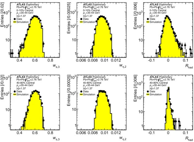
Figure 2: Comparisons of distributions of three photon identification variables from data (black points) with full simulation results (yellow histogram), for photons with
pT =35
−44.1 GeV and
|η|< 1.37.
Events from the 0-10% centrality interval are shown in the top row, while those from the 40-80% interval are shown in the bottom row.
centrality dependence of the means of the shape variables are well described by the simulation, within the limited statistics of the electron and positron sample.
Comparisons of shower shape variables between data and simulation are used to validate the use of the simulation for determining efficiency and background contamination correction factors. Fig. 2 shows three typical distributions of shape variables for data from the 0-10% and 40-80% centrality intervals, each compared with the corresponding quantities in simulation. For these distributions, the candidate photons pass a stringent photon selection (described below in Section 5) and have a reconstructed trans- verse energy in the range 35 <
pT< 44.1 GeV (after UE subtraction) and
|η|< 1.37. The simulated distributions are all normalized to the number of counts in the corresponding data histogram. The data contains some admixture of neutral hadrons, so complete agreement should not be expected in the full distributions.
The electromagnetic energy trigger e
fficiency has been checked using a sample of minimum bias
data, where the primary triggers did not select on particular high-p
Tactivity. In this sample, events were
triggered based on either a coincidence in the two ZDCs or a total of 50 GeV or more deposited in the
ATLAS calorimeter system. Using these the probability for an identified photon to match to a first level
trigger “region of interest” of 16 GeV or more with a
∆R< 0.15 between the reconstructed photon and
the trigger cluster, reaches 100% just above photon
pT =20 GeV, a result similar to that obtained in
ppcollisions. To be above the turn-on region, the minimum
pTrequired in this analysis is 22 GeV.
Photons are selected for offline analysis using a variation of the “tight” criteria developed for the photon analysis in
ppcollisions. Specific intervals are defined on all nine shower shape variables de- fined above, and are implemented in a
pT-independent, but η-dependent scheme. The intervals for each variable have been defined by choosing the range for each variable to contain 95% of the distribution of matched photons with
pT =40
−60 GeV in the 0-10% centrality interval.
The admixture of converted photons, which depends on the amount of material in front of the elec- tromagnetic calorimeter, and thus the pseudorapidity of the photon, is not accounted for in the analysis, but is confirmed by the good agreement of the shower shape variable distributions between data and sim- ulation, discussed previously. Converted photons tend to have wider showers than unconverted photons, and so substantially broaden the shower shape variables.
In order to estimate the hadron background from jets, a “non-tight” selection criterion has been defined, which is particularly sensitive to neutral hadron decays. For this selection, a photon candidate is required to fail at least one of the more stringent selections in the first calorimeter layer except for w
s,tot(w
s,3,
Fside,
Eratioand
∆E). These reversed selections enhance the probability of accepting neutralhadron decays from jets, via candidates with a clear double shower structure (via
Eratioand
∆E) as wellas candidates in which the two showers may have merged (via w
s,3,
Fside) [12].
While the photon energy calibration is the same as used for
ppcollisions, based in part on measure- ments of
Zbosons decaying into an electron and positron, and validated with
Z →``
+γ events [28], the admixture of converted and unconverted photons leads to a small underestimate of the photon en- ergy on average in Pb
+Pb events, since the energy of converted photon clusters are typically recon- structed in a slightly larger region in the calorimeter. This is quantified by the photon energy scale
“closure”, the mean fractional difference between the reconstructed and truth photon transverse energies, (
precoT − ptruthT)/
ptruthT ≡∆pT/
pT, obtained from simulation. For matched photons, the average deviation from the truth photon
pTis the largest at low photon
pTand is typically within 1% for
pT> 44.1 GeV.
The fractional energy resolution, determined by calculating the RMS of
∆pT/p
truthTin small intervals in truth
pT, ranges from 4% at
pT =22 GeV to 1.5% at
pT =200 GeV for
|η|< 1.37 and from 5% to 3%
for 1.52 <
|η|< 2.37. The net e
ffects of the deviation of the photon energy scale from the true value, and from energy resolution, are corrected using the bin-by-bin unfolding factors described below.
In order to further reject clusters arising from hadronic fragments of jets, the calorimeter is also used to measure an isolation energy for each photon candidate,
ET,iso. The isolation energy is the sum of transverse energies in calorimeter cells (including hadronic and electromagnetic sections) in a cone
R<
Risoaround the photon axis. The photon energy is removed by excluding a central core of cells in a region corresponding to 5×7 cells in the second layer of the EM calorimeter. In previous ATLAS
ppanalyses [12, 13], the cone size was chosen to be
Riso =0.4, while in this heavy ion analysis, the cone is chosen to be slightly smaller,
Riso=0.3, to reduce the sensitivity to UE fluctuations. Furthermore, the analysis presented here also uses a less restrictive isolation criterion
ET,iso< 6 GeV (with
Riso =0.3), as compared to the criterion used in the
ppanalyses
ET,iso< 3 GeV with (R
iso =0.4) [12, 13]. An additional correction, based on simulations and parametrized by the photon transverse energy and η, is then applied to the calculated isolation energy to minimize the e
ffects of photon shower leakage into the isolation cone. It amounts to a few percent of the photon transverse energy.
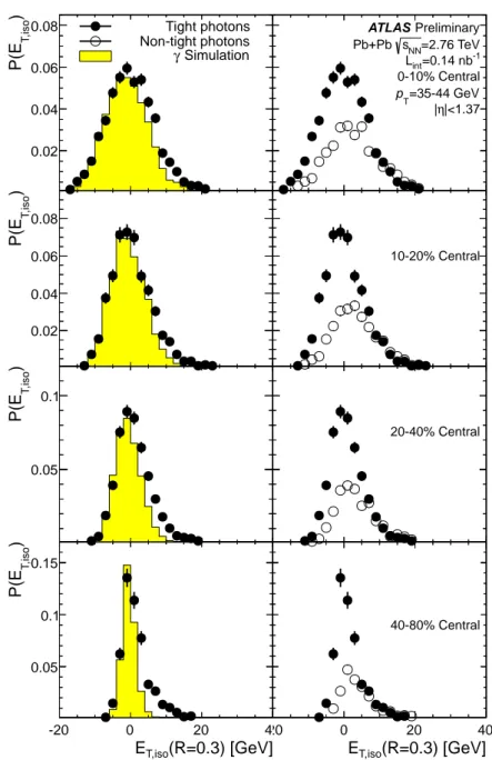
The left column of Fig. 3 shows the distributions of
ET,isofor tight photons candidates with
pT =35
−44.1 GeV as a function of collision centrality, compared with simulated distributions. The data
and simulations have been normalized so the integrals of
ET,iso< 0, where no significant background
from jets is expected, are the same. Both the simulated and measured
ET,isodistributions grow noticeably
wider with increasing centrality; as the UE subtraction only accounts for the mean energy in an η interval,
local fluctuations are still present. Furthermore, in the data, an enhancement on the
ET,iso> 0 side of
these distributions is expected from the jet background. The
ET,isodisrtibution for a sample enhanced in
backgrounds is shown in the right column of Fig 3, which shows the isolation distribution for the non-
(R=0.3) [GeV]
T,iso
E
-20 0 20 40
) T,isoP(E
0.05 0.1 0.15
(R=0.3) [GeV]
T,iso
E
-20 0 20 40
) T,isoP(E
0.05 0.1 0.15
40-80% Central
(R=0.3) [GeV]
T,iso
-20 0E 20 40
) T,isoP(E
0.05 0.1
(R=0.3) [GeV]
T,iso
-20 0E 20 40
) T,isoP(E
0.05 0.1
20-40% Central
(R=0.3) [GeV]
T,iso
-20 0E 20 40
) T,isoP(E
0.02 0.04 0.06 0.08
(R=0.3) [GeV]
T,iso
-20 0E 20 40
) T,isoP(E
0.02 0.04 0.06 0.08
10-20% Central
(R=0.3) [GeV]
T,iso
E
-20 0 20 40
) T,isoP(E
0.02 0.04 0.06
0.08 Tight photons
Non-tight photons Simulation γ
(R=0.3) [GeV]
T,iso
E
-20 0 20 40
) T,isoP(E
0.02 0.04 0.06
0.08 ATLAS Preliminary
=2.76 TeV sNN
Pb+Pb
=0.14 nb-1
Lint
0-10% Central
=35-44 GeV pT
|<1.37 η
|
Figure 3: Distributions of photon isolation transverse energy in a
Riso =0.3 cone for the four centrality bins in data (black points, normalized by the number of events and by the histogram bin width), for photons with
pT =35
−44.1 GeV. In the left column simulations (yellow histogram) are shown normalize to the data so that the integrals for
ET,isoare the same. The corresponding sample of non-tight photon candidates, normalized to the distribution of tight photons for
ET,iso> 8 GeV is shown overlaid on the tight photon data in the right column to illustrate the source of the photons with large
ET,iso. Please see main text for further detail.
tight candidates in the same
pTinterval. For larger values of
ET,iso, the non-tight sample has the same
distribution as for the tight photon candidates. The distributions are normalized to the integral of the
tight photon candidate distribution in the region
ET,iso> 8 GeV. As the width of
ET,isovaries with FCal
ΣET, the impact of the di
fference in the
ΣETdistributions from data and simulation has been studied
=0.3) [GeV]
(Riso
ET
0 10 20 30
Tight Non-tight
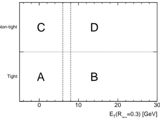
A B
C D
Figure 4: Illustration of the double side-band approach, showing the two axes for partitioning photon candidates: region A is the “signal region” (tight and isolated photons) for which efficiencies are defined, region B contains tight, non-isolated photons, region C contains non-tight isolated photons, and region D contains non-tight and non-isolated photons.
and found to be negligible compared with other uncertainties. Hence, no reweighting is applied to the simulated events. To account for any systematic difference between the distributions in data and MC, the cut on the isolation is varied in both data and MC as described in Sec. 8.
In this measurement, only the highest
pTphoton is considered, since far less than 1% of events with a reconstructed photon are expected to have a second hard photon, and the overall rate of additional tight, isolated photon candidates in the data was found to be less than 1% relative to that for the highest-energy photon candidates. After application of the tight selection and an isolation criterion of
ET,iso< 6 GeV to the 0-80% centrality sample, there are approximately 51,000 candidates with
pT> 22 GeV within
|η|
< 1.37 and 26,000 candidates within 1.52 <
|η|< 2.37.
6 Yield extraction
The kinematic intervals used in this analysis are defined as follows. For each centrality bin, as described above, the photon kinematic phase space is divided into intervals in photon η and
pT. The regions in η are 0 <
|η|< 0.8, 0.8 <
|η|< 1.37, 1.52 <
|η|< 2.01, and 2.01 <
|η|< 2.37. The
pTintervals used are logarithmic, and are
pT =17.5
−22 GeV (only used in Monte Carlo simulations), 22
−27.8 GeV, 27.8
−35.0 GeV, 35.0
−44.1 GeV, 44.1
−55.6 GeV, 55.6
−70.0 GeV, 70.0
−88.2 GeV, 88.2
−111.1 GeV, 111.1
−140.0 GeV, 140.0
−176.4 GeV, 176.4
−222.2 GeV, and 222.2
−280.0 GeV.
The technique used to subtract the background from jets from the measured yield of photon can- didates is the “double side-band” method, already used by ATLAS in Refs. [12, 13]. In this method, photon candidates are partitioned along two dimensions, illustrated in Fig. 4. The horizontal axis is the isolation energy within a chosen isolation cone size. The vertical axis divides the sample into two re- gions, the first one for photons that pass the tight selection outlined above, and the second for non-tight photon candidates that fail at least one of the more stringent selection criteria. The motivation for this partitioning is to find candidates which satisfy most of the criteria for being photons, but which have an enhanced probability of stemming from hadrons from jet fragmentation.
The four regions are labelled A,B,C and D and correspond to the four categories expected for recon-
structed photons:
• A: tight, isolated photons:
Primary signal region where a large fraction of all truth photons would appear, after applying a truth-level isolation criterion.
• B: tight, non-isolated photons:
The region in which photons are produced in the vicinity of a jet, or an UE fluctuation in the case of a heavy ion collision
• C: non-tight, isolated photons:
The region which contains a combination of isolated neutral hadron decays within jets, as well as real photons which have a shower shape fluctuation that fails the tight selection. The contribution from the latter increases with increasing collision centrality.
• D: non-tight, non-isolated photons:
The region populated primarily by neutral hadron decays within jets, but which can have a small admixture of photons that both fail tight selection and are accompanied by a local upward fluctuation of the UE.
Non-tight and non-isolated photons are used to estimate the contribution from jets in the signal region A. This is appropriate provided there is no correlation between the axes for background photon candidates, e.g. that the probability of a neutral hadron decay passing the tight or non-tight selection criteria is not dependent on whether or not it is isolated. This has been checked using a sample of high-
pTphoton candidates from simulated jet events, which do not have a truth photon present, and within the large statistical uncertainties of the sample, the
ET,isodistributions for tight and non-tight background photons are the same. If there is no leakage of signal from region A to the other non-signal regions (B, C and D), the double side-band approach utilizes the ratio of counts in C to D to extrapolate the measured number of counts in region B to correct the measured number of counts in region A, i.e.
Nsig =NAobs−NobsB NCobs
NDobs
(2)
Leakage of signal into the background regions needs to be removed before attempting to extrapolate into the signal region. A set of “leakage factors”,
ci, are calculated to extrapolate the number of signal events in region A into the other regions.
NsigA =NAobs−
NobsB −cBNAsig
NCobs−cCNAsig
NobsD −cDNsigA
(3) The leakage factors are calculated using simulations as
ci = Nisig/N
sigA, where
NAsigis the number of simulated tight, isolated photons.
Equation 3 is solved via the quadratic formula for
NsigA, the number of signal photons. The physical root is taken as the background-corrected yield,
NAsig. The statistical uncertainties in the number of signal photons for each centrality, η and
pTinterval were evaluated with the following pseudo-experiment method. The equation is solved 5000 times, each time sampling the parameters
NobsA−Dfrom a multinomial distribution with the probabilities given by the observed values divided by their sum, and the parameters
NA−Dsigfrom a Gaussian distribution with the observed value assumed to be the mean of the distribution and the uncertainty taken from the simulated distributions. The Gaussian standard deviation of the pseudo- experiments is taken as the statistical uncertainty on the mean.
The e
fficiency, defined for tight, isolated photons relative to primary truth photons with a parton- level isolation in a cone of
R=0.3 around the photon direction of less that 6 GeV, is classified into three categories:
• Reconstruction efficiency:
This is the probability that a photon is reconstructed with greater
than 10 GeV. In the heavy ion reconstruction, the losses primarily stem from a subset of photon
[GeV]
pT
photon
30 40 102 2×10²
Efficiency
0 0.2 0.4 0.6 0.8 1
|<2.37 η 40-80%, 1.52<|
[GeV]
pT
photon
30 4050 102 2×10²
Efficiency
0 0.2 0.4 0.6 0.8 1
|<2.37 η 20-40%, 1.52<|
[GeV]
pT
photon
30 4050 102 2×10²
Efficiency
0 0.2 0.4 0.6 0.8 1
|<2.37 η 10-20%, 1.52<|
[GeV]
pT
photon
30 4050 102 2×10²
Efficiency
0 0.2 0.4 0.6 0.8 1
|<2.37 η 0-10%, 1.52<|
[GeV]
pT
photon
30 40 102 2×10²
Efficiency
0 0.2 0.4 0.6 0.8 1
|<1.37 η 40-80%, |
[GeV]
pT
photon
30 40 102 2×10²
Efficiency
0 0.2 0.4 0.6 0.8 1
|<1.37 η 20-40%, |
[GeV]
pT
photon
30 40 102 2×10²
Efficiency
0 0.2 0.4 0.6 0.8 1
|<1.37 η 10-20%, |
[GeV]
pT
photon
30 40 102 2×10²
Efficiency
0 0.2 0.4 0.6 0.8 1
|<1.37 η 0-10%, |
Pb+Pb ATLAS
Simulation Preliminary
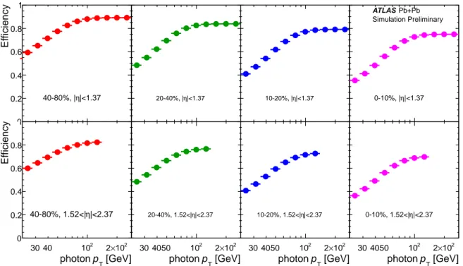
Figure 5: Total photon efficiency as a function of photon
pTand event centrality averaged over
|η|< 1.37 (top row) and 1.52 <
|η|< 2.37 (bottom row).The e
fficiencies are smoothed using a Fermi function.
No systematic uncertainties are shown, but the systematic uncertainties pertaining to the efficiencies are discussed in Sec. 8.
conversions, in which the energy of the electron and positron is not contained within a region small enough to be reconstructed by the standard algorithms. This factor is typically around 95% near η
=0 and decreases to 90% at forward angles, and is found to be approximately constant as a function of transverse momentum for the range measured here.
• Identification efficiency:
This is the probability that a reconstructed photon (according to the previous definition) passes tight identification selections.
• Isolation efficiency:
This is the probability that a photon which would be reconstructed and pass identification selections, also passes the chosen isolation selection. The large fluctuations from the UE in heavy ion collisions can lead to an individual photon being found in the non-isolated region with a non-trivial probability. While leakage into region B also depends weakly on photon
pT, the overall magnitude of the isolation e
fficiency primarily reflects the standard deviation of the isolation energy distribution.
These e
fficiencies are defined in such a way that the “total e
fficiency”
totis simply the product of these three factors. Fig. 5 shows the total e
fficiency for each centrality and η interval.
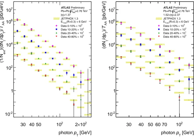
7 Photon yields
For each interval in
pT, η and centrality (
C), the per-event yield of leading photons is defined as 1
Nevt
(
C)
dNγ d pT(
pT, η,
C)= NsigA U(pT, η,
C)Nevt
(
C)
tot(
pT, η,
C)∆
pT(4)
where
NAsigis the background-subtracted yield in region A (determined using the method described in the previous section),
Uis a factor that corrects for the bin migration due to the finite photon energy resolution and any residual bias in the photon energy scale,
totis the above-mentioned total efficiency,
Nevtis the number of minimum bias events in centrality interval
C, and∆pTis the width of the transverse momentum interval.
The final photon yields are extracted using the tight selections described in Section 5, an isolation cone radius of
Riso =0.3 and isolation transverse energy selection of
ET,iso< 6 GeV to define region A, and
ET,iso> 8 GeV to define region B. Regions C and D are defined using the same isolation energy selections, but for photon candidates that satisfy the non-tight selection. For the 0-10% centrality interval, the 6 GeV isolation selection has an efficiency of about 85-90%.
The leakage factors are calculated in the simulation with this choice of side-band regions from re- constructed photons in the simulation matched to truth photons. In the 40-80% centrality interval, for
|η|
< 1.37 and for
pT =22
−280 GeV,
cBis generally less than 0.01,
cCranges from 0.13 to 0.02, and
cDis less than 0.003. In the 0-10% centrality interval and over the same
pTrange,
cBranges from 0.07 to 0.10,
cCranges from 0.2 to 0.02, and
cDranges from 0.02 to 0.005. Except for
cB, which reflects the different isolation distributions in peripheral and central events, the leakage factors are of similar scale as found in
pp. This procedure results in an estimate ofNAsig, the background-corrected yield of signal photons in the measured sample. The purity of the photon sample in the double side-band method is then defined as
P= NAsig/N
Aobs. For kinematic regions in which the side-band statistics are small, particularly at the highest
pTvalues, the side-bands are populated by measuring the ratio of each side-band (B,C and D) to region A as a function of
pTand extrapolating linearly in 1/p
T, utilizing all of the available data up to
pT =200 GeV. The statistical uncertainty on these data points include the uncertainties of the fits.
It should be noted that the purity merely represents the outcome of the side-band subtraction procedure, and is not used as an independent correction factor.
The extracted values of
Pare shown in Fig. 6 as a function of transverse momentum in the four measured centrality intervals and two η intervals. Values of
P> 1 can arise when the number of events in the background regions is low, but they are all consistent with values
P ≤1, within the statistical uncertainties. In all four centrality and both η intervals, the purity increases from about 0.5 at the lowest
pTinterval to about 0.9 at the highest
pTintervals. The points to the right of the dotted line utilize the extrapolation procedure discussed in the previous paragraph.
To correct for the residual non-closure of the photon energy scale, stemming primarily from con- verted photons treated as unconverted, as well as the photon energy resolution, the data are unfolded using the bin-by-bin correction technique [12] to generate the correction factors
U. The correction fac-tors deviate from unity by about 10% in the lowest
pTinterval (22.1-28 GeV), but decrease rapidly over the next two bins and are typically within 4% over the full
pTrange in both η ranges.
A sample of simulated
Wboson decays to electron or positron and a neutrino have been used to study the residual contamination expected as a fraction of the expected photon rates. From this, it has been estimated that a non-negligible background can be expected in the 35 <
pT< 44.1 GeV interval with a magnitude of about 5% in the forward pseudorapidity region, and about 3% in the central region. These small corrections have been applied to the final yields, with an absolute systematic uncertainty of 1%.
8 Systematic uncertainties
Several sources of systematic uncertainty have been estimated by varying the assumptions applied to the
analysis, and then redoing the full analysis chain to test the level to which the data and simulations agree
in detail. At high
pT, the
pTdependence of most of the variations is generally found to be modest, so
the overall effect on the photon yield is determined for each set of variations by a fit to each of constant
over
pT =44.1
−111.1 GeV. The largest variation is selected from each set, and applied symmetrically
[GeV]
pT
photon
30 40 102 2×10²
Purity
0 0.5 1
|<2.37 η 40-80%, 1.52<|
[GeV]
pT
photon
30 4050 102 2×10²
Purity
0 0.5 1
|<2.37 η 20-40%, 1.52<|
[GeV]
pT
photon
30 4050 102 2×10²
Purity
0 0.5 1
|<2.37 η 10-20%, 1.52<|
[GeV]
pT
photon
30 4050 102 2×10²
Purity
0 0.5 1
|<2.37 η 0-10%, 1.52<|
[GeV]
pT
photon
30 40 102 2×10²
Purity
0 0.5 1
|<1.37 η 40-80%, |
[GeV]
pT
photon
30 40 102 2×10²
Purity
0 0.5 1
|<1.37 η 20-40%, |
[GeV]
pT
photon
30 40 102 2×10²
Purity
0 0.5 1
|<1.37 η 10-20%, |
[GeV]
pT
photon
30 40 102 2×10²
Purity
0 0.5 1
|<1.37 η 0-10%, |
Preliminary ATLAS
= 2.76 TeV sNN
Pb+Pb = 0.14 nb-1
Lint
Figure 6: Photon purity as a function collision centrality (left to right) and photon
pT, for photons measured in
|η|< 1.37 (top row) and 1.52 <
|η|< 2.37 (bottom row).
to all points above 44.1 GeV. However, for
pT =22
−44.1 GeV, the e
ffects of the di
fferent variations are typically larger than at higher
pT, so they are determined separately.
• Tight selection: To assess the sensitivity to the diff
erences between data and simulations in the shower shape variable distributions, the definition of the tight selection criteria have been varied, using an alternate scheme based on a small modification to the selections used for the
ppenvi- ronment, and the entire analysis repeated all the way through, reevaluating all leakage, e
fficiency, energy scale, and isolation corrections. Variations on the final yields range from 3–10%, depending on the centrality and η interval under consideration.
• Isolation criteria: The cone radius has been changed toR=
0.4, the isolation energy selection has been varied up and down by 2 GeV, and the shower leakage corrections are varied. The effects on the final yields are typically below 10%, with some larger changes in specific
pT, η and centrality intervals. This accounts for possible differences between the isolation distribution for prompt photons between data and simulation.
• Non-tight selection: In order to assess the sensitivity to the choice of non-tight criteria, which
allow background events into the analysis, the non-tight definition has been changed from four reversed conditions, to five (adding w
s,tot) and two (using just
Fsideand w
s,3). The variation is typically less than 10% for
pT< 44.1 GeV and less than 5% for
pT> 44.1 GeV range.
• Purity: The purity is sensitive to the specific choices of the tight selection scheme and the isolation