ATLAS-CONF-2012-051 28May2012
ATLAS NOTE
ATLAS-CONF-2012-051
May 28, 2012
Measurement of high p
Tisolated prompt photons in lead-lead collisions at
√ s
NN= 2.76 TeV with the ATLAS detector at the LHC
The ATLAS Collaboration
Abstract
Prompt photons are a powerful tool in heavy ion collisions. Their production rates pro- vide access to the initial state PDFs, which are expected to be modified by nuclear e
ffects.
They also provide a means to calibrate the expected energy of jets that are produced in the medium, and thus are a tool to probe the physics of jet quenching more precisely both through jet spectra and fragmentation properties. The ATLAS detector measures photons with its hermetic, longitudinally segmented calorimeter, which gives excellent spatial and energy resolution, and detailed information about the shower shape of each measured pho- ton. This gives significant rejection against the expected background from neutral pions in jets. Rejection against jet fragmentation products is further enhanced by isolation criteria, which can be based on calorimeter energy or the presence of high
pTtracks. First results on the spectra of isolated prompt photons from approximately 133
µb−1of lead-lead data are shown, as a function of transverse momentum and centrality. The measured spectra are compared to expectations from perturbative QCD calculations.
c
Copyright 2012 CERN for the benefit of the ATLAS Collaboration.
Reproduction of this article or parts of it is allowed as specified in the CC-BY-3.0 license.
1 Introduction
While jet quenching at the Large Hadron Collider (LHC) was discovered using di-jet asymmetry dis- tributions [1], the detailed physical mechanism is still not understood. One of the limiting factors in understanding jet quenching is having a proper calibration of the initial jet energy. Di-jet measurements are limited by the fact that one does not know whether or not the leading jet was itself quenched. Single jet measurements [2, 3] are themselves limited by the fact that, at a given measured jet
pT, they are integrating over a range of initial unquenched jet energies. Replacing one of the jets with a penetrating probe, such as a photon or electroweak boson (W or Z), o
ffers the possibility of calibrating the energy of the initial jet. This was first proposed by Wang and collaborators in Ref. [4].
As an important prerequisite to making photon-jet measurements, it is essential to measure photon rates in heavy ion collisions. In general, “prompt” photons are those that do not arise from hadron decays.
Prompt photons are themselves expected to have two primary sources. The first is direct emission, which proceeds via quark-gluon Compton scattering
qg → qγor quark-antiquark annihilation
qq → gγ. Thesecond is the “fragmentation” contribution, from the production of a single hard photon during parton fragmentation. At leading order, there is a meaningful distinction between the two processes, but at next-to-leading-order (NLO) the two cannot be unambiguously separated. In order to remove QCD background events from di-jet processes, as well as fragmentation photons, an “isolation” criterion is typically applied within a cone of a well-defined radius relative to the photon direction. The isolation energy requirement can be applied as a fraction of the photon energy, or as a constant energy threshold.
In either case, these can be applied consistently to a QCD calculation such that prompt photon rates can be calculated. At high
pT, photon rates are expected to be modified by nuclear e
ffects on the nucleon PDFs, as well as by jet-medium interactions (see e.g. Ref.[5]).
Prompt photon rates have been measured extensively in proton-proton collisions, from the CERN ISR [6, 7] to the CERN SppS [8] and to the Fermilab Tevatron[9, 10]. Both of the large LHC experiments, ATLAS [11, 12] and CMS [13] have measured isolated prompt photons in the early
√s =7 TeV proton-
proton data. In nearly all cases, good agreement has been found with perturbative QCD calculations at next to leading order, which are typically calculated using the JETPHOX package [14, 15]. In lower- energy heavy ion collisions, the PHENIX experiment performed measurements of direct photon rates in gold-gold collisions at
√sNN =
200 GeV [16].
Hard process rates in heavy ion collisions generally scale as follows, for any particular process (la- beled “X” here):
NX =LAAσAAtothNcolliσppX
σpptot
(1)
In this equation,
LAAis the heavy ion integrated luminosity,
σAAtotis the total inelastic lead-lead cross section (calculated to be 7.6 b using Glauber Monte Carlo code [17, 18]),
hNcolliis the mean number of binary collisions,
σppXis the cross section for subprocess
Xin proton-proton collisions, and
σpptotis the total inelastic proton-proton cross section. Given that
LAA×σAAtotis the number of inelastic events (N
evt), while
hNcolli/σpptotis simply the mean nuclear thickness function
hTAAi, one can define a suppressionvariable as:
RAA =
(N
X/Nevt)
TAAσppX
(2)
This allows the straightforward comparison of yields in heavy ion collisions, normalized by the initial parton flux, to cross sections measured in proton-proton data and calculated using standard event and process generators. CMS performed the first measurement of isolated prompt photon rates in both proton- proton as well as lead-lead collisions, at the nucleon-nucleon CM energy of
√s =
2.76 TeV [19]. They
found rates consistent with a scaling with the number of binary collisions, and thus found
RAAvalues
consistent with unity for all centrality and
pTranges considered.
In this work, isolated prompt photons are measured in lead-lead collisions with the ATLAS detector, making use of its large-acceptance, longitudinally segmented calorimeter. Yields per event are measured averaged over
|η| <1.3 and as a function of photon
pTfrom 45-200 GeV. Comparisons with previous data as well as NLO QCD calculations are also presented.
2 Experimental setup
2.1 ATLAS detector
The ATLAS detector is described in detail in Ref. [20]. The ATLAS inner detector is comprised of three major subsystems: the pixel detector, the semiconductor detector (SCT) and the transition radiation tracker (TRT), which cover full azimuth and pseudorapidity
1out to
|η|=2.5. The pixel detector consists of three layers, at radii of 50.5, 88.5 and 122.5 mm, arranged in cylindrical layers in the barrel region (|η|
<2) and three disks in the endcap region. The SCT is comprised of four cylindrical layers of double- sided silicon detectors at radii ranging from 299 to 514 mm in the barrel region, and 9 disks in the endcap region (of which a typical particle trajectory crosses four). The TRT covers the larger radii from 563 to 1066 mm with 72 layers of straw tubes, of which a particle typically leaves signals in about 40 straws.
The entire detector is immersed in a 2 T axial magnetic field and allows tracking up to
|η|=2.5 using the pixel and SCT, and
|η|=2.0 using the TRT.
The ATLAS calorimeter is a large-acceptance, longitudinally-segmented sampling calorimeter cov- ering out to
|η| =4.9 with electromagnetic and hadronic sections. The electromagnetic section is a lead-liquid argon sampling calorimeter with an accordion geometry. It is divided into the barrel region, covering
|η|<1.475, and two endcap regions, covering 1.375
<|η|<3.2. The calorimeter has three pri- mary longitudinal sections, called “layers”. The first sampling layer is 3 to 5 radiation lengths deep and is segmented into fine “strips” of size
∆η=0.003− 0.006 (depending on
η), which allows the discrimina-tion of photons from the two-photon decays of
π0and
ηmesons. The second layer is 17 radiation lengths thick, sampling the majority of an electromagnetic shower, and has cells of size
∆η×∆φ=0.025
×0.025.
The third layer has a material depth ranging from 4 to 15 radiation lengths and is used to catch the tails of high energy electromagnetic showers. In front of the strip layer, a presampler is used to correct for energy loss in front of the calorimeter within the region
|η| <1.8. In test beam environments and in typical proton-proton collisions, the calorimeter is found to have a sampling term of 10-17%/
√E[GeV].
The total material in front of the electromagnetic calorimeter ranges from 2.5 to 6 radiation lengths as a function of pseudorapidity, except the transition region between the barrel and endcap regions, in which the material is up to 11.5 radiation lengths.
The hadronic calorimeter section is located radially just after the electromagnetic calorimeter. Within
|η|<
1.7, it is a sampling calorimeter of steel and scintillator tiles, with a depth of 7.4 hadronic interaction lengths. In the endcap region it is copper and liquid argon with a depth of 9 interaction lengths.
2.2 Photon trigger
The sample of events used in this analysis was collected using the first level calorimeter trigger of the ATLAS experiment [21]. This is a hardware trigger which sums up electromagnetic energy in towers of size
∆η×∆φ =0.1
×0.1, which is substantially coarser than the electromagnetic calorimeter. A sliding window of size 0.2
×0.2 was used to find electromagnetic clusters by looking for local maxima and, keeping only those with energy in two adjacent cells (i.e. regions with a size of either 0.2
×0.1 or
1ATLAS uses a right-handed coordinate system with its origin at the nominal interaction point (IP) in the centre of the detector and thez-axis along the beam pipe. Thex-axis points from the IP to the centre of the LHC ring, and theyaxis points upward. Cylindrical coordinates (r, φ) are used in the transverse plane,φbeing the azimuthal angle around the beam pipe. The pseudorapidity is defined in terms of the polar angleθasη=−ln tan(θ/2).
0.1
×0.2) exceeding a programmable threshold. The trigger with the lowest
pTthreshold that was not prescaled for the duration of the 2011 heavy ion run had a threshold of 16 GeV, which has been found to be 100% efficient for photons above 20 GeV.
3 Estimation of the underlying event
In order to reconstruct photons in the context of a heavy ion collision, the large background from the underlying event (UE) is subtracted from each event. This is performed during the heavy ion jet recon- struction, as explained in detail in Ref.[22], whose description is closely followed here.
This procedure is done in several iterative steps. A first estimate of the underlying event average transverse energy density,
ρi(η), is evaluated for each calorimeter layer
iin intervals of
ηof width
∆η=0.1 using all cells in each calorimeter layer, within the given
ηinterval excluding those within “seed” jets.
In the first subtraction step, the seeds are defined to be jets reconstructed using the anti-k
t[23] algorithm with
R =0.2 which have at least one tower with
ET >3 GeV and which have a ratio of the maximum to the mean tower energy of at least 4. The presence of elliptic flow in lead-lead collisions leads to a 2v
2cos 2(φ
−Ψ2)
modulation on the UE, where v
2is the second coefficient in a Fourier decomposition of the azimuthal variation of the UE particle or energy density, and the event plane angle,
Ψ2, points in the direction of the largest upward modulation in the event.
The techniques outlined in [24, 25] are used to measure
Ψ2on an event-by-event basis, using the event plane defined by the ATLAS forward calorimeter (FCal):
Ψ2 =
1 2 tan
−1
X
k
wkETk
sin (2φ
k)
Xk
wkETk
cos (2φ
k)
,
(3)
where
kruns over cells in the FCal,
φkrepresents the cell azimuthal angle, and
wkrepresent per-cell weights empirically determined to smooth the
Ψ2distribution. An
η-averaged v2was measured sepa- rately for each calorimeter layer according to
v
2i= Xj∈i
ETj
cos
h2
φj−Ψ2
i X
j∈i
ETj
,
(4)
where
jruns over all cells in layer
i. The UE-subtracted cell energies were calculated according to ETsubj = ETj−Ajρi(η
j)
1
+2v
2icos
h2
φj−Ψ2
i,
(5)
where
ETj,
ηj,
φjand
Ajrepresent the cell
ET,
ηand
φpositions, and area, respectively, for cells,
j,in layer
i. The kinematics forR =0.2 jets generated in this first subtraction step were calculated via a four-vector sum of all (assumed massless) cells contained within the jets using the
ETvalues obtained from Eq. 5.
The second subtraction step starts with the definition of a new set of seeds using a combination of
R =0.2 calorimeter jets from the first subtraction step, each with
ET >25 GeV, and jets formed from inner detector tracks, using anti-k
Twith
R =0.4, with
pT >10 GeV. Using this new set of seeds, a new estimate of the UE,
ρ0i(η), is calculated excluding cells within
∆R<0.4 of the new seed jets, where
∆R= q
(η
cell−ηjet)
2+(φ
cell−φjet)
2. New v
2ivalues, v
20i
, were also calculated excluding all cells within
∆η=
0.4 of any of the new seed jets. This exclusion largely eliminates distortions of the calorimeter v
2measurement in events containing high-
pTjets.
4 Photon reconstruction
Once the mean energy
ρiand v
2ivalues are evaluated in each layer, excluding all seeds from the aver- aging, the background subtraction is then applied to the original cell energies using Eq. 5 but with
ρiand v
2ireplaced by the new values,
ρ0i(η) and v
20i. This procedure provides a new set of “subtracted”
cells, from which the mean underlying event has been removed, as well as the large-scale modulation of elliptic flow. The residual deposited energies stem primarily from three sources: jets, photons/electrons, and background fluctuations (possibly including higher order flow harmonics). It should be noted that while it is straightforward to estimate a mean energy as a function of
η, it is at present not possible tomake further subtraction of more localized structures. Thus, fluctuations are an essential aspect of the photon analysis in the heavy ion data.
Acting upon the subtracted cells, the ATLAS photon reconstruction [26] is seeded by clusters of at least 2.5 GeV found using a sliding window algorithm applied to the second sampling layer of the electromagnetic calorimeter, which typically samples over 50% of the deposited photon energy. In the dense environment of the heavy ion collision, the photon conversion recovery procedure is not performed, due to the overwhelming number of combinatoric pairs in more central collisions. However, a substantial fraction of converted photons are still reconstructed by the photon algorithm, as at these high energies, the electron and positron are typically close together as they reach the calorimeter, while their tracks typically originate at a radius too large to be well-reconstructed by the tracking algorithm which is optimized for heavy ion collisions. Thus, the photon sample analyzed here is a mix of converted and unconverted photons, as will be directly illustrated below.
The energy measurement is made using all three layers of the electromagnetic calorimeter and the presampler, with a size corresponding to 3
×5 (in
ηand
φ) cells in the second layer (each being0.025
×0.025). An energy calibration is applied to each shower to account for both its lateral leakage (outside the nominal window) and longitudinal leakage (into the cryostat and hadronic calorimeter) [26].
This window size is used in the proton-proton analysis for unconverted photons, while it is used for all photons in this analysis of heavy ion data, leading to a slight degradation in performance when applied to converted photons.
4.1 Photon shower shape variables
The fine-grained, longitudinally segmented calorimeter used in ATLAS allows detailed characterization of the shape of each photon shower, providing tools to reject jets and hadrons, while maintaining high e
fficiency for the photons themselves. In this analysis, nine shower-shape variables are used, all of which have been used extensively in previous ATLAS publications, particularly the measurement of prompt photon spectra as a function of pseudorapidity [11, 12].
The primary shape variables used can be broadly classified by which sampling layer is used.
The second sampling is used to measure
• Rη
, the ratio of energies deposited in a 3
×7 (η
×φ) window to that deposited in a 7×7 window, in units of the second layer cell size.
• wη,2
, the root-mean-square width of the energy distribution of the cluster in the second layer in the
ηdirection
• Rφ
, the ratio of energies deposited in a 3
×3 (η
×φ) window in the second layer to that depositedin a 3
×7 window, in units of the second layer cell size.
The hadronic calorimeter is used to measure the fraction of shower energy that reaches the hadronic
calorimeter:
• Rhad
, the ratio of transverse energy measured in the hadronic calorimeter to the transverse energy of the photon cluster.
• Rhad1
, the ratio of transverse energy measured in the first sampling layer of the hadronic calorimeter to the transverse energy of the photon cluster.
The cut is applied on
Rhad1when
|η|<0.8 or
|η|>1.37 while it is applied to
Rhadotherwise.
Finally, cuts are applied in five other quantities measured in the high granularity strip layer, to reject neutral meson decays from jets. In this finely-segmented layer a search is applied for multiple maxima from neutral hadron electromagnetic decays:
• ws,tot
, the total RMS of the transverse energy distribution in the
ηdirection in the first sampling
“strip” layer
• ws,3
, the RMS width of the three “core” strips including and surrounding the cluster maximum in the strip layer
• Fside
, the fraction of transverse energy in seven first-layer strips surrounding the cluster maximum, not contained in the three core strips (i.e. (E(±3)
−E(±1))/E(±1))• Eratio
, the asymmetry between the transverse energies in the first and second maxima in the strip layer
• ∆E, the diff
erence between the transverse energy of the first maximum, and the minimum cell transverse energy between the first two maxima.
In general, it has been found in ATLAS that the shower shape variables measured in data di
ffer slightly, but significantly, from the Monte Carlo calculations [11]. To account for these differences, a set of correction factors has been developed to account for small shifts in the distributions. This analysis uses the standard shift factors obtained by comparing
ppsimulations to the same quantities in the data, with no modification for the heavy ion environment. It is found that the broad features of the distributions agree quite well between data and simulation, except in the regions where di-jet background is expected.
4.2 Photon isolation energy
In order to further reject clusters arising from hadronic fragments of jets, particularly neutral mesons, the calorimeter is also used to measure an isolation energy for each photon candidate,
ET(R
iso). The isolation energy is the sum of transverse energies in calorimeter cells (including hadronic and electromagnetic sections) in a cone
R = p∆η2+ ∆φ2 < Riso
around the photon axis. The photon energy is removed by excluding a central core of cells in a region corresponding to 5
×7 cells in the second layer of the EM calorimeter. In previous ATLAS pp analyses [11, 12], the cone size was chosen to be
Riso=0.4, while in this heavy ion analysis, the cone is chosen to be slightly smaller,
Riso =0.3, to reduce the sensitivity to underlying event fluctuations. The analysis presented here also uses a less restrictive isolation criterion
ET(R
iso =0.3)
<6 GeV, as compared to the criterion used in the pp analyses
ET(R
iso =0.4)
<3 GeV [11, 12].
A standard correction based on a fraction of the photon energy is applied to the calculated isolation
energy to remove photon shower leakage into the isolation cone. However, it is found that a small
(approximately 2%) leakage of the photon energy contaminates the isolation cone energy in the most
peripheral events. At present, no correction is applied for this. However, a systematic uncertainty based
on this residual leakage is assigned as a function of centrality (see below).
[TeV]
ET
Σ FCal
0 1 2 3
Counts/Event [1/TeV]
10-7
10-5
10-3
10-1
10
40-80% 20-40% 10-20% 0-10%
Preliminary ATLAS
=2.76 TeV sNN
Pb+Pb Minimum bias 16 GeV trigger 40 GeV tight photons
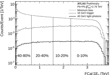
Figure 1: Distribution of FCal
ΣET, at the 2011 energy scale, with centrality bins indicated. The dotted line shows the distribution for minimum bias data, the dashed line shows the distribution of events that trigger the 16 GeV level 1 trigger, and the solid line shows the distribution for photon candidates with
ET >40 GeV satisfying tight selection cuts (see section 10.3).
5 Centrality selection
The centrality of each heavy ion collision is determined using the sum of the transverse energy in all cells in the forward calorimeter (3.1
< |η| <4.9), at the electromagnetic scale, FCal
ΣET. The trigger and event selection were studied in detail in the 2010 data sample [24] and it was found that it kept 98
±2% of the total inelastic cross section. The increased luminosity of the 2011 heavy ion run necessitated a more sophisticated trigger strategy, including more restrictive triggers in the most peripheral events. However, it was found that the FCal
ΣETdistributions in the 2011 data match those measured in 2010 to a high degree of precision, after accounting for a 4.1% scaling applied to the new data reflecting improved understanding of the energy calibrations. For this analysis, the data have been divided into 4 centrality intervals, covering the 0-10%, 10-20%, 20-40% and 40-80% most central events. In this convention, the 0-10% interval has the highest multiplicities, and the 40-80% the lowest. These bins are shown in Figure 1.
The FCal
ΣETdistribution is shown for three types of events. The top distribution (dotted line) is for the recorded minimum bias events. The dashed line shows the distribution for events that satisfy the 16 GeV level 1 electromagnetic cluster trigger. It is evident that these events are biased toward more central events, as might be expected from the scaling with the number of binary collisions. Finally, the solid line shows the distributions for photon candidates with
ET >40 GeV, and that satisfy the “tight” selection cuts explained in Section 10.3.
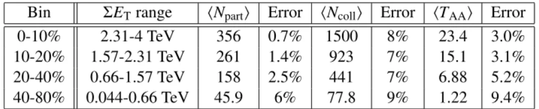
Table 1 collects all of the centrality-related information used in this analysis. It specifies the FCal
ΣETranges for each bin, the mean number of participants per bin with its total systematic uncertainty,
the mean number of binary collisions with its total uncertainty, and finally the mean nuclear thickness
hTAAi. The geometric quantities are calculated as described in Ref. [29] using a Glauber Monte Carlo
calculation, with a simple implementation of the ATLAS FCal response. One finds smaller uncertainties
of the mean nuclear thickness since it is the ratio of
Ncoll, which scales with
σNN, and
σNNitself.
Bin
ΣETrange
hNpartiError
hNcolliError
hTAAiError
0-10% 2.31-4 TeV 356 0.7% 1500 8% 23.4 3.0%
10-20% 1.57-2.31 TeV 261 1.4% 923 7% 15.1 3.1%
20-40% 0.66-1.57 TeV 158 2.5% 441 7% 6.88 5.2%
40-80% 0.044-0.66 TeV 45.9 6% 77.8 9% 1.22 9.4%
Table 1: Centrality bins used in this analysis, tabulating the percentage range, the
ΣETrange (in 2011), the average number of participants (hN
parti) and binary collisions (hNcolli) and the relative error on thesequantities.
6 Simulation data samples
For the extraction of photon performance parameters (e
fficiencies, photon energy scale, isolation prop- erties), a set of 450,000 photon+jet events using the ATLAS MC11 tune of PYTHIA 6.4 at
√s =
2.76 TeV, is overlaid on minimum-bias HIJING events, which are referred-to as “HIJING+PYTHIA” sam- ples. The HIJING events are modified after initial generation to include angular modulations as a func- tion of centrality, transverse momentum and pseudorapidity, parametrized from ATLAS measurements of the second through sixth Fourier components of the angular distributions relative to the event plane measured in the FCal [27]. The sample is divided equally into three subsamples based on requiring a minimum transverse momentum for the outgoing primary photon. The first has
pT >17 GeV, the second has
pT >35 GeV and the third
pT>70 GeV. The generated samples are fully simulated using GEANT4 and digitized to produce simulated raw data files, that are reconstructed and analyzed exactly as is done for experimental data.
In the HIJING+PYTHIA sample, the FCal
ΣEThas been scaled up by 1.081 to best match the measured and simulated distributions. This is to ensure a comparison of equivalent levels of activity in the barrel region where the analysis is performed, and detailed comparisons of fluctuations in small regions have already been performed by ATLAS [28], which validate this procedure.
7 Comparison of photon candidates in data and simulation
7.1 Photon shower shape variables
Comparisons of shower shape variables are used to validate the use of the Monte Carlo for determining
efficiency and background contamination correction factors. Figure 2 shows three typical examples of
shape variables for data from the 0-10% centrality bin, compared with Monte Carlo calculations. In all
cases, photon clusters passing tight cuts with reconstructed transverse energy greater than 40 GeV (after
UE subtraction) and
|η|<1.3 are shown. These distributions are all normalized by the number of counts
in each distribution, separately for data and Monte Carlo, and divided by the bin width.
ws,3
0 0.2 0.4 0.6 0.8 1
Normalized counts
10-1
1 10
Preliminary ATLAS Data Simulation Converted Unconverted 0-10% Central
η,2
w
0.005 0.01 0.015
Normalized counts
10 102
103 ATLAS Preliminary
Rhad1
-0.1 -0.05 0 0.05 0.1
Normalized counts
10-1
1 10 102
Preliminary ATLAS
ws,3
0 0.2 0.4 0.6 0.8 1
Normalized counts
10-2
10-1
1
10 ATLAS Preliminary Data
Simulation Converted Unconverted 40-80% Central
η,2
w
0.005 0.01 0.015
Normalized counts
1 10 102
103 ATLAS Preliminary
Rhad1
-0.1 -0.05 0 0.05 0.1
Normalized counts
10-1
1 10 102
Preliminary ATLAS
Figure 2: Comparisons of three photon identification variables from data (black points) with full sim- ulation results. 0-10% central events are shown in the top row, while 40-80% central is shown on the bottom. The simulation is shown both fully integrated (yellow) and broken out into contributions from unconverted photons (red histogram) and converted photons (blue histogram).
8 Theoretical predictions
While the MC11 PYTHIA samples are used for corrections within small phase space bins, they also pro- vide a prediction of the photon spectrum at leading order. For next-to-leading order (NLO) calculations, the JETPHOX package is used [15], which has been successfully compared to data from the Tevatron and LHC. JETPHOX provides access to all modern PDFs and calculates both direct production as well as photons from fragmentation processes, with an implementation of an isolation cut built into the cal- culations. The calculations shown in this work use the CTEQ6.6 PDFs, with no nuclear modification, and require less than 6 GeV isolation energy in a cone of
Riso =0.3 relative to the photon direction.
Uncertainties are estimated by simultaneously varying the renormalization and initial and final state fac-
torization scales by a factor of two, relative to the baseline result, assuming
µR = µI = µF = pTphoton.
This coherent variation of the renormalization and initial and final state factorization scales by a factor
of two varies the JETPHOX yield up and down by about 13%, independent of
pTwithin the numerical
accuracy of the calculations.
9 Collision data selection
9.1 Event selection
The data sample analyzed here is from the 2011 LHC heavy ion run, colliding lead nuclei at
√sNN =
2.76 TeV. After requiring the 16 GeV Level 1 electromagnetic cluster trigger, which is sensitive in particular to both electrons and photons, events were selected which contained a reconstructed photon or electron object with a cluster transverse energy of at least 40 GeV. Events were then further analyzed if they satisfied a set of quality cuts: The event had to be taken during a period when the detector was found to be working properly, leaving an integrated luminoisty of about
Lint=133
µb−1for this analysis, after the exclusion of several runs. Both sets of Minimum Bias Trigger Scintillators (covering 2.09
<|η|<3.84) have to have a well reconstructed time signal, and a relative time between the two counters of less than 5 ns. Finally, a good vertex is required to be reconstructed in the ATLAS detector, to reject background events from e.g. cosmic rays. While ATLAS recorded about 150 million events out of the nearly one billion delivered minimum bias collisions in the 2011 heavy ion run, the photon sample only contains less than 250k events, and only a fraction of these were photons passing the quality cuts outlined below.
9.2 Estimating number of sampled events
In this measurement, yields are presented per minimum bias collision, which are estimated using the total integrated luminosity, measured using the ATLAS luminosity detectors [30]. The luminosity has been calculated using a coincidence rate of the two LUCID detectors, with special dead-time free elec- tronics, with an algorithm that accounted for accidental rates [31]. Converting the measured luminosity to the total number of minimum bias events requires a measurement of event counts for the minimum bias sample. The conversion factor from measured luminosity to the total number of events has been measured by counting the total number of sampled minimum-bias events of centrality 80% and above, and correcting for prescale factors, with a precision of better than 1%, as established by comparing data taken at widely separated time intervals throughout the heavy ion run. This procedure gives the number of minimum bias events in the most-central 80% events to be
Nevt =786×10
6events, with an uncertainty of less than 1%.
9.3 Isolation energy distributions
As described above, the isolation energy
ET(R
iso) is the sum of transverse energies in calorimeter cells in a cone around the photon axis, excluding the photon itself, which is defined as the central core of cells in a region corresponding to 5×7 cells in the second layer of the EM calorimeter. The distance of the outer radius of the cone from the photon axis in the
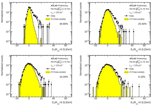
ηplane can be anywhere from 0.2 to 0.4. Figure 3 shows the distributions of
ET(R
iso=0.3) for the data as a function of collision centrality, compared with simulated distributions, normalized in the region
ET(R
iso =0.3)
<0. Both data and MC distributions grow noticeably wider with increasing centrality, as the background subtraction is only able to subtract the mean energy in an
ηinterval, removing reconstructed jets, so local fluctuations are still preserved.
Furthermore, in the data, an enhancement on the
ET(R
iso=0.3)
>0 side of these distributions is expected from di-jet background. Still it is observed that the isolation distributions in data and simulation vary in a similar fashion, especially in the region of negative isolation energy.
Given that the width of the distribution varies with the eventwise FCal
ΣET, growing slowly with
centrality, it is important to check the e
ffect of the di
ffering distributions of
ΣETin data and MC, since
the MC is not weighted to resemble the solid curve in Figure 1. The ratio between the minimum bias
distribution and the triggered distribution is approximately linear in
ΣET. To assess the effect of this
di
fference, distributions were studied with and without scaling the distributions by
ΣET. The largest
=0.3) [GeV]
(Riso
ET
-20 0 20 40 60
Normalized counts
10-4
10-3
10-2
10-1
1
40-80%
Preliminary ATLAS
=2.76 TeV sNN
Pb+Pb b-1
µ = 133 Lint
Data PYTHIA+HIJING
=0.3) [GeV]
(Riso
ET
-20 0 20 40 60
Normalized counts
10-4
10-3
10-2
10-1
1
20-40%
Preliminary ATLAS
=2.76 TeV sNN
Pb+Pb b-1
µ = 133 Lint
Data PYTHIA+HIJING
=0.3) [GeV]
(Riso
ET
-20 0 20 40 60
Normalized counts
10-4
10-3
10-2
10-1
1
10-20%
Preliminary ATLAS
=2.76 TeV sNN
Pb+Pb b-1
µ = 133 Lint
Data PYTHIA+HIJING
=0.3) [GeV]
(Riso
ET
-20 0 20 40 60
Normalized counts
10-4
10-3
10-2
10-1
1
0-10%
Preliminary ATLAS
=2.76 TeV sNN
Pb+Pb b-1
µ = 133 Lint
Data PYTHIA+HIJING
Figure 3: Distributions of photon isolation energy in a
Riso =0.3 cone for the four centrality bins in data (black points) and for MC (yellow histogram), normalized for negative
ET(R
iso =0.3) values. The differences at large values of
ET(R
iso=0.3) can be attributed to the presence of jet contamination in the data, which is not present in the MC sample.
difference was with the most peripheral bin, where the width (estimated by a Gaussian fit) was 14%
larger in the weighted case. However, the fraction of MC events over a fixed cut of 6 GeV (explained below) is 5% in the unweighted distribution and 6% in the weighted distribution. Given the small e
ffect found in these estimates, reweighting is not used in the final analysis, and the expected effects on the extracted yields are far smaller than the final stated systematic uncertainties, discussed below.
10 Photon trigger and reconstruction performance
10.1 Kinematic bins
The kinematic intervals used in this analysis are defined as follows. For each centrality bin, as described above, the photon kinematic phase space is divided into intervals in photon
ηand
pT. For the presentation of final yields, photons are integrated over
|η| <1.3 but some corrections are made separately in four intervals, [−1.3,
−0.8),[−0.8,0.0),[0.0, 0.8] and (0.8, 1.3]. Within each
ηinterval, there are eight ranges in
pT, 45-50 GeV, 50-60 GeV, 60-70 GeV, 70-80 GeV, 80-100 GeV, 100-120 GeV, 120-140 GeV, and 140-200 GeV.
10.2 Photon trigger e ffi ciency
The trigger efficiency has been checked using a sample of minimum bias data, where the primary triggers
did not select on particular high-
pTactivity. In this sample, events were triggered based on either a
coincidence in the zero degree calorimeters (ZDCs), which measure neutral particles with
|η| >8.3
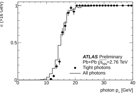
or a total of 50 GeV or more deposited in the calorimeter system. Figure 4 shows the probability for
[GeV]
photon pT
0 10 20 30 40
(>16 GeV)∈
0 0.5 1
Preliminary ATLAS
=2.76 TeV sNN
Pb+Pb Tight photons All photons
Figure 4: Trigger e
fficiency for events with photon candidates, based on minimum bias data, given as the ratio of the number of “HI tight” photons (points) and all photon candidates (histogram) where an associated 16 GeV electromagnetic energy trigger was satisfied at level 1, relative to all recorded events.
fully identified photons (after background subtraction) (black points) or inclusive photon candidates (histogram) to match to a L1 “region of interest” of 16 GeV or more with a
∆R <0.15 between the reconstructed photon and the trigger cluster. It is found that the e
fficiency curve in both cases reaches 100% just above photon
pT =20 GeV, similar to that found in pp collisions.
10.3 Photon selection cuts
Photons are selected for this analysis using the “tight” criteria developed for the photon analysis in proton-proton collisions. Cut intervals are defined on all nine shower shape variables defined above, and are implemented in a
pT-independent, but
η-dependent scheme. The cuts used in this analysis are “HItight” cuts, defined as a minimal set of changes to the standard set of tight cuts used for unconverted pho- tons in the proton-proton analysis. These had been optimized in proton-proton collisions as a function of
η, reflecting the presence of different detector geometries and di
fferent numbers of radiation lengths in front of the calorimeter. For the heavy ion analysis, as small a set of the cuts as possible were re- laxed to maintain good performance and background rejection, while avoiding too strong of a centrality dependence, which can be induced by the e
ffect of fluctuations on several of the variables,
∆Eand
Rφin particular. As two examples, the upper cut on
∆Ewas increased from approximately 100 MeV to 300 MeV, while the minimum cut on
Rφwas reduced to 0.7 from approximately 0.9. The admixture of converted photons, which depends on the amount of material in front of the electromagnetic calorimeter, and thus the pseudorapidity of the photon, is not accounted for in the analysis, but is checked by means of comparison of data with Monte Carlo.
After application of “HI tight” cuts to the 0-80% centrality sample, but before applying isolation
requirements, there are 6435 photon candidates with
pT >45 GeV and within
|η|<1.3.
photon reco pT
0 50 100 150 200
T/pTp∆
-0.02 -0.015 -0.01 -0.005 0 0.005
-0.8 η -1.3 <
Preliminary ATLAS
HIJING+PYTHIA
photon reco pT
0 50 100 150 200
T/pTp∆
-0.02 -0.015 -0.01 -0.005 0 0.005
Preliminary ATLAS
HIJING+PYTHIA
< 0 η -0.8 <
photon reco pT
0 50 100 150 200
T/pTp∆
-0.02 -0.015 -0.01 -0.005 0 0.005
Preliminary ATLAS
HIJING+PYTHIA
< 0.8 η 0 <
photon reco pT
0 50 100 150 200
T/pTp∆
-0.02 -0.015 -0.01 -0.005 0 0.005
Preliminary ATLAS
HIJING+PYTHIA
< 1.3 η 0.8 <
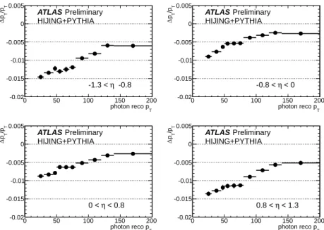
Figure 5: Photon energy scale
∆pT/pTderived from the HIJING+PYTHIA sample as a function of reconstructed photon
pT, applied as a correction to the reconstructed photon energy.
10.4 Photon energy scale
While the photon energy calibration is the same as used for
ppcollisions, based on measurements of
Zbosons decaying into an electron and positron [26], the mixing of converted and unconverted photons leads to a small underestimate of the photon energy on average. This section gives a more detailed look at the photon energy scale, the fractional di
fference between the reconstructed and truth photon transverse energies, (p
Treco−pTtruth)/p
Treco. Reconstructed tight and isolated photons (our nominal signal sample) are matched to primary truth photons when they are within
R = p∆φ2+ ∆η2 <
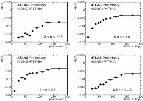
0.2 relative to each other. For these photons, the average correction to the photon energy scale is calculated for the four pseudorapidity bins described above in section 10.1). To illustrate the performance of the reconstruction, Figure 5 shows the dependence of this correction on the truth photon
pT. Figure 6 shows the dependence of this correction on reconstructed photon
pT, which is used to apply this correction to the measured photon candidates. It was checked that there are no significant di
fferences between peripheral and central events, and so centrality-integrated average corrections are used.
10.5 Energy resolution
The fractional energy resolution determined by Gaussian fits to
∆pT/pTin 4 GeV intervals in
pTis shown in Figure 7 for peripheral (40-80%) and central (0-10%) events, and for two bins in
|η|. They are fit withthe form
σ(pT)/p
T = qp20+
(p
1/√pT
)
2+(
p2/pT)
2. The sampling term
p1for central events is found
to be 10-12% in both pseudorapidity bins. While these fits are not used in the analysis, it is useful to get
a sense of the precision of the ATLAS electromagnetic calorimeter for measuring photon energies.
photon truth pT
0 50 100 150 200
T/pTp∆
-0.02 -0.015 -0.01 -0.005 0 0.005
< -0.8 η -1.3 <
Preliminary ATLAS
HIJING+PYTHIA
photon truth pT
0 50 100 150 200
T/pTp∆
-0.02 -0.015 -0.01 -0.005 0 0.005
Preliminary ATLAS
HIJING+PYTHIA
< 0 η -0.8 <
photon truth pT
0 50 100 150 200
T/pTp∆
-0.02 -0.015 -0.01 -0.005 0 0.005
Preliminary ATLAS
HIJING+PYTHIA
< 0.8 η 0 <
photon truth pT
0 50 100 150 200
T/pTp∆
-0.02 -0.015 -0.01 -0.005 0 0.005
Preliminary ATLAS
HIJING+PYTHIA
< 1.3 η 0.8 <
Figure 6: Photon energy scale
∆pT/pTderived from the HIJING
+PYTHIA sample as a function of reconstructed photon
pT, applied as a correction to the truth photon energy.
[GeV]
photon truth pT
50 100 150
T)/p T(pσ
0 0.02 0.04 0.06
Preliminary ATLAS
HIJING+PYTHIA
=2.76 TeV sNN
|<0.8 η
| 40-80%
0-10%
|<1.3 η 0.8<|
40-80%
0-10%
Figure 7: Photon resolution
σ(pT)/
pTfrom simulation, for 0-10% central events (closed symbols), 40-
80% peripheral events (open symbols),
|η|<0.8 (circles) and 0.8
<|η|<1.3 (squares).
11 Yield extraction
11.1 Double sideband technique
The main goal of this note is to measure the fully-corrected spectrum of photons for each centrality bin.
This involves removal of background from di-jet events and correction for the photon e
fficiency. Correc- tions to the spectral shape from the photon energy resolution are found to be small and are not included in this analysis. The technique used for background subtraction is the so-called “double sideband method”.
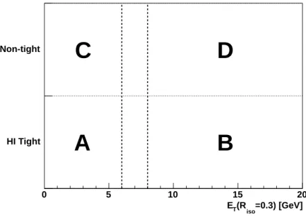
In this approach, already used by ATLAS in Refs. [11] and [12], photon candidates are binned on two axes, illustrated in Figure 8. The horizontal axis is the isolation energy within a chosen isolation cone size. The vertical axis is essentially a two-valued one, where the first bin is for photons that pass the
“tight” cuts outlined above, while the other bin is for “non-tight” candidates, photons that fail at least one of the more stringent cuts. The idea is to find candidates which satisfy most of the criteria for being photons, but which have an enhanced probability of being from jet fragments.
=0.3) [GeV]
(Riso
ET
0 5 10 15 20
HI Tight Non-tight
A B
C D
Figure 8: Illustration of the double sideband approach, showing the two axes for binning photon can- didates: region A is the “signal region” (tight and isolated photons) for which efficiencies are defined, region B contains tight, non-isolated photons, region C contains non-tight isolated photons, and region D contains non-tight and non-isolated photons.
The four regions are labelled A,B,C and D and correspond to four well-defined categories:
• A: tight, isolated photons:
This is the primary signal region where a well-defined fraction of all truth photons would appear, after applying a truth-level isolation criterion.
• B: tight, non-isolated photons:
These are photons which happen to be in the vicinity of a jet, or an underlying event fluctuation in the case of a heavy ion collision
• C: non-tight, isolated photons:
These are a combination of isolated jet fragments, as well as real
photons which have a shower shape fluctuation that fails the tight cuts. The contribution from the
latter increases with increasing collision centrality.
• D: non-tight, non-isolated photons:
This region should primarily be background, since they are candidates which are neither narrow photons, nor ones which are in isolated regions.
The non-tight photons are used to estimate the contribution from jets in the signal region A. This works provided there is essentially no correlation between the axes, i.e. that it is not the isolated nature of a cluster which tends to make it pass tight cuts. If this is rigorously the case, and if there is no leakage of signal from region A to the other non-signal regions (B, C and D), then the double sideband approach suggests that one can use the ratio of counts in C to D to extrapolate the measured number of counts in region B to correct the measured number of counts in region A, i.e.
Nsig =NAobs−NobsB NCobs
NDobs
(6)
If there is any leakage of signal into the background regions, then these must be removed systematically before attempting to use them to extrapolate into the signal region. A set of “leakage factors”,
ci, are calculated to extrapolate the number of signal events in region A into the other regions.
NsigA =NAobs−
NobsB −cBNAsig
NCobs−cCNAsig
NobsD −cDNsigA
(7) The leakage factors are calculated using the simulated PYTHIA sample as
ci= Nisig/NAsig. In the 40-80%
centrality interval and from
pT =40 to 200 GeV,
cBranges from 0.005 to 0.04,
cCranges from 0.06 to 0.02, and
cDis less than 0.003. In the 0-10% centrality interval and over the same
pTrange,
cBranges from 0.16 to 0.24,
cCranges from 0.06 to 0.01, and
cDranges from 0.01 to 0.005. Except for
cB, which reflects the very different isolation distributions in peripheral and central events, the isolation factors are of similar scale.
In practice, Equation 7 is solved numerically using the Brent root solver implemented into ROOT [32].
In order to calculate the statistical uncertainty for each centrality and
pTinterval, the equation is solved 5000 times, each time sampling the eight parameters (N
Aobs−NobsD,
NsigA −NsigD) from a Poisson distribu- tion with the observed value assumed to be the mean of the distribution. The mean of a Gaussian fit to the distribution of
Nsigis taken as the background-corrected yield, while Gaussian standard deviation is taken as the statistical error on the mean.
11.2 Photon e ffi ciencies
The final conversion of the measured yield into a yield per event, and ultimately into
RAA, requires several more factors: the total number of events in each centrality sample, and a reconstruction efficiency including all known e
ffects. The e
fficiencies are defined for “HI tight”, isolated photons relative to all PYTHIA photons with an isolation energy in a cone of
Riso =0.3 around the photon direction of less than 6 GeV. This selection at the truth particle level removes about 1.5% of the photon sample.
Once the truth photons are properly defined, the needed e
fficiency corrections are categorized into three broad classes:
• Reconstruction efficiency:
This is the probability that a photon is reconstructed with 90% or more of its truth energy. In the heavy ion reconstruction, the losses primarily stem from a subset of photon conversions, in which the energy of the electron and positron is not contained within a region small enough to be reconstructed by the standard algorithms. This factor is typically around 95% and is found to be constant as a function of transverse momentum for the range measured here.
• Identification efficiency:
This is the probability that a reconstructed photon (according to the
previous definition) passes “tight” identification cuts.
[GeV]
photon pT
0 50 100 150 200
Efficiency
0 0.2 0.4 0.6 0.8 1
Preliminary ATLAS
40-80%
∈ Photon ID
20-40%
∈ Photon ID
10-20%
∈ Photon ID
0-10%
∈ Photon ID
40-80%
∈ Total
20-40%
∈ Total
10-20%
∈ Total
0-10%
∈ Total
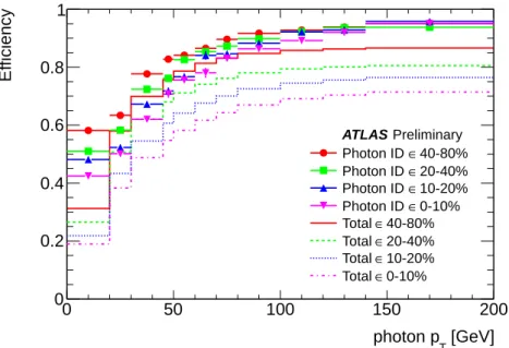
Figure 9: Photon reconstruction e
fficiency as a function of photon
pTand event centrality averaged over
|η| <1.3, based on MC calculations performed in four subintervals in
η. The points indicate theidentification efficiency, without the contribution from the isolation requirement. The solid lines indicate the smoothed total e
fficiency used to correct the measured photon yield.
• Isolation efficiency:
This is the probability that a photon which would be reconstructed and pass identification cuts, also passes the chosen isolation cut. While this is not performed the
ppanalysis, where the fluctuations of the isolation energy are well below the chosen isolation cut, the large fluctuations from the underlying event in heavy ion collisions can lead to an individual photon being found in the non-isolated region. While leakage into region B also depends on photon
pT, the isolation e
fficiency primarily reflects the standard deviation of the isolation energy distribution.
These e
fficiencies are defined in such a way that the “total e
fficiency”
tot– the probability that a photon would be reconstructed AND identified AND isolated – is simply the product of these three factors.
These are assessed using the standard “HI tight” definitions and an isolation cut of 6 GeV within
Riso =0.3 around the photon direction. Figure 9 shows the product of the reconstruction and identification efficiency (points) and the total efficiency (solid lines).
12 Photon yields
In this section, the double sideband technique is applied to extract the photon yield per minimum bias event (1/N
evt)dN/
pT(
pT,c), divided by the mean nuclear thicknesshTAAi(which scales as the number of binary collisions). The photon yield is defined as
1
NevtdNγ
d pT
(p
T,c)= NAsigtot ×Nevt×∆pT
(8)
where
NAsigis the background-subtracted yield in region A,
totis the abovementioned total e
fficiency,
Nevtis the number of events in centrality bin
c,∆pTis the width of the transverse momentum interval,
and
hTAAiis the average nuclear thickness for that bin. Each bin requires a small correction to account
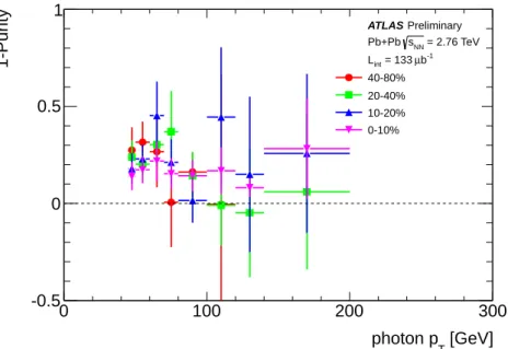
[GeV]
photon pT
0 100 200 300
1-Purity
-0.5 0 0.5 1
Preliminary ATLAS
= 2.76 TeV sNN
Pb+Pb b-1
µ = 133 Lint
40-80%
20-40%
10-20%
0-10%