ATLAS-CONF-2013-016 07March2013
ATLAS NOTE
ATLAS-CONF-2013-016
March 4, 2013
Search for non-pointing photons in the diphoton and E
Tmissfinal state in
√ s = 7 TeV proton–proton collisions using the ATLAS detector
The ATLAS Collaboration
Abstract
A search has been performed for photons originating in the decay of a neutral long- lived particle, exploiting the capabilities of the ATLAS electromagnetic calorimeter to make precise measurements of the flight direction of photons, as well as the calorimeter’s excellent time resolution. The search has been made in the diphoton plus missing transverse energy final state, using the full data sample of 4.8 fb
−1of 7 TeV proton–proton collisions collected in 2011 with the ATLAS detector at the LHC. No excess is observed above the background expected from Standard Model processes. The results are used to set exclusion limits in the context of Gauge Mediated Supersymmetry Breaking models, with the lightest neutralino being the next-to-lightest supersymmetric particle and decaying with a finite lifetime into a photon and gravitino.
c Copyright 2013 CERN for the benefit of the ATLAS Collaboration.
Reproduction of this article or parts of it is allowed as specified in the CC-BY-3.0 license.
1 Introduction
Supersymmetry (SUSY) [1–9], a theoretically well-motivated candidate for physics beyond the Standard Model (SM), predicts the existence of a new SUSY partner (sparticle) for each of the SM particles, with identical quantum numbers except differing by half a unit of spin. In R-parity conserving SUSY mod- els [10–14], these sparticles could be produced in pairs in proton–proton (pp) collisions at the CERN Large Hadron Collider (LHC), and would decay in cascades involving other sparticles and SM parti- cles until the lightest SUSY particle (LSP), which is stable, is produced. In Gauge Mediated Super- symmetry Breaking (GMSB) models [15–20], the LSP is the gravitino ( ˜
G). GMSB phenomenology islargely determined by the properties of the next-to-lightest supersymmetric particle (NLSP). The results of this analysis are presented in the context of the so-called Snowmass Points and Slopes parameter set 8 (SPS8) [21], which describes a set of minimal GMSB models with the lightest neutralino ( ˜
χ01) as the NLSP. In the SPS8 set of models, the effective scale of SUSY breaking, denoted
Λ, is a free parameter.In addition, the ˜
χ01proper decay length,
cτ( ˜χ01), is a free parameter of the theory.
In the SPS8 models, the dominant decay mode of the NLSP is ˜
χ01 → γ +G. Previous ATLAS˜ analyses have assumed prompt NLSP decays, with
cτ( ˜χ01)
<0.1 mm, and therefore searched for an excess production of diphoton events which, due to the escaping gravitinos, exhibit significant missing transverse momentum (E
missT). The latest such ATLAS results [22] use the full 2011 dataset and, within the context of SPS8 models, exclude values of
Λ<196 TeV, corresponding to
m( ˜χ01)
>280 GeV, at 95%
CL. The limits on SPS8 models are less stringent in the case of a longer-lived NLSP. For example, recent CMS 95% CL limits [23], obtained using the
EmissTspectrum of events with at least three jets and one or two photons, coupled with measurements of the photon arrival time, require
m( ˜χ01)
>220 GeV for
cτ( ˜χ01) values up to 500 mm.
The analysis reported in this paper uses the full data sample of 4.8 fb
−1of 7 TeV
ppcollisions collected in 2011 with the ATLAS detector at the LHC, and considers the scenario where the ˜
χ01has a finite lifetime and can travel some distance from its production point before decaying. The search is performed in an inclusive sample of candidate diphoton
+EmissTevents, which is a final state with well understood trigger and background contributions.
The long-lived NLSP scenario introduces the possibility of a decay photon being produced after a finite delay and with a flight direction that does not point back to the primary vertex (PV) of the event.
The analysis searches for such “non-pointing photons” by exploiting the fine segmentation of the ATLAS electromagnetic (EM) calorimeter to measure the flight direction of photons. The variable used as a measure of the degree of non-pointing of the photon is
zDCA, the difference between the
z-coordinate1of the photon extrapolated back to its distance-of-closest-approach (DCA) to the beamline (ie.
x= y=0) and
zPV, the
z-coordinate of the PV. The search for non-pointing photons is then performed by fitting theshape of the
zDCAdistribution obtained for photons in the signal region, defined as diphoton events with
EmissT >75 GeV, to a combination of templates which describe the
zDCAdistribution for the expected signal and background events. In addition, the excellent time resolution of the calorimeter is exploited to measure the arrival times of the photons, providing a cross check of the results.
1ATLAS uses a right-handed coordinate system with its origin at the nominal interaction point (IP) in the centre of the detector and thez-axis along the beam pipe. Thex-axis points from the IP to the centre of the LHC ring, and theyaxis points upward. Cylindrical coordinates (r, φ) are used in the transverse plane,φbeing the azimuthal angle around the beam pipe. The pseudorapidity is defined in terms of the polar angleθasη=−ln tan(θ/2).
2 The ATLAS Detector
The ATLAS detector [24] covers nearly the entire solid angle around the collision point, and consists of an inner tracking detector surrounded by a solenoid, EM and hadronic calorimeters, and a muon spectrometer incorporating three large toroidal magnet systems. The ATLAS inner-detector system (ID) is immersed in a 2 T axial magnetic field, provided by a thin superconducting solenoid located before the calorimeters, and provides charged particle tracking in the pseudorapidity range
|η| <2.5. The ID consists of three detector subsystems, beginning closest to the beamline with the high-granularity silicon pixel detector, followed at larger radii by the silicon microstrip tracker and then the straw-tube based transition radiation tracker. The ID allows an accurate reconstruction of tracks from the primary
ppcollision and precise determination of the location of the PV. The ID also identifies tracks from secondary vertices, permitting the efficient identification of photons which convert to electron-positron pairs as they pass through the detector material.
This analysis relies heavily on the capabilities of the ATLAS calorimeter system, which covers the pseudorapidity range
|η| <4.9. EM calorimetry is provided by barrel (
|η| <1.475) and end-cap (1.375
<|η|<3.2) lead/ liquid-argon (LAr) EM sampling calorimeters. An additional thin LAr presam- pler covering
|η|<1.8 allows corrections for energy losses in material upstream of the EM calorimeters.
Hadronic calorimetry is provided by a steel/scintillating-tile calorimeter, segmented into three barrel structures within
|η| <1.7, and two copper/LAr hadronic end-cap calorimeters. The solid angle cov- erage is completed with forward copper/LAr and tungsten/LAr calorimeter modules optimised for EM and hadronic measurements, respectively. Outside the ATLAS calorimeters lies the muon spectrometer, which identifies and measures the deflection of muons up to
|η| <2.7, in a magnetic field generated by superconducting air-core toroidal magnet systems.
2.1 Pointing Resolution
The EM calorimeter is finely segmented, and consists of three longitudinal layers. The first layer uses highly granular “strips” segmented in the
ηdirection, designed to allow efficient discrimination between single photon showers and two overlapping showers originating from the decay of a
π0meson. The sec- ond layer collects most of the energy deposited in the calorimeter by EM showers initiated by electrons or photons. Very high energy showers can leave significant energy deposits in the third layer, which can also be used to correct for energy leakage beyond the EM calorimeter. By measuring precisely the centroids of the EM shower in the first and second layers, the flight direction of photons can be determined. In the ATLAS
H →γγanalysis [25] that contributed to the discovery of a Higgs-like particle, this capability of the EM calorimeter was used to help choose the PV from which the two photons originated, thereby improving the diphoton invariant mass resolution and sensitivity of the search. The analysis described in this paper uses the measurement of the photon flight direction to search for photons that do not point back to the PV, which is chosen to be the vertex with the greatest sum of the square of the transverse momenta of all associated tracks. The angular resolution of the EM calorimeter’s measurement of the flight direction of prompt photons is of the order of 60 mrad/
√E, where E is the energy measured in GeV. This angular precision corresponds, in the EM barrel calorimeter, to a resolution on
zDCAof the order of 15 mm for prompt photons with energies in the range of 50–100 GeV. Given the geometry, the
zDCAresolution is worse for photons reconstructed in the end-cap calorimeters, so the pointing analysis is restricted to photon candidates in the EM barrel calorimeter.
While the geometry of the EM calorimeter has been optimised for detecting particles which point
back near the nominal interaction point at the center of the detector (ie.
x = y = z =0), the fine
segmentation allows good pointing performance to be achieved over a wide range of photon impact
angles. Figure 1 shows, as a function of
|zDCA|, the expected pointing resolution for SPS8 signal photons,
obtained by fitting to a gaussian the difference between the value of
zDCAobtained from the calorimeter
measurement and the truth information. The pointing resolution degrades with increasing
|zDCA|, but remains much smaller than
|zDCA|in the region where our signal candidates lie.
The calorimeter pointing performance has been verified in data by using the finite spread of the LHC collision region along the
z-axis. Superimposed on Figure 1 is the pointing resolution achieved for asample of electrons from
Z →eeevents, where the distance,
zPV, between the PV and the nominal center of the detector (ie.
x=y=z=0) serves the role of
zDCA. In this case, the pointing resolution is obtained by fitting to a gaussian the difference between
zPV, as determined with high precision using tracking information, and the calorimeter measurement of the origin of the electron, along the beamline. Figure 1 shows that similar pointing performance is observed for photons and for electrons, as expected given their similar EM shower developments. This similarity validates the use of a sample of electrons from
Z →eeevents to study the pointing performance for photons. The expected pointing performance for electrons in a Monte Carlo (MC) sample of
Z → eeevents is also shown on Figure 1, and is consistent with the electron data. The agreement between MC and data over the range of values which can be accessed in the data gives confidence in the extrapolation using MC to the larger deviations from pointing characteristic of the signal photons.
| [mm]
|z
DCA0 100 200 300 400 500 600 700 800
Pointing Resolution [mm]
20 40 60 80 100 120 140 160
SPS8 Signal MC ee (2011 Data)
→ Z
ee (MC)
→ Z
Preliminary ATLAS
Data 2011
Ldt = 4.8 fb
-1∫
= 7 TeV, s
Figure 1: Pointing resolution obtained for EM showers in the ATLAS LAr EM barrel calorimeter. Su- perimposed are the results of data and MC samples of electrons from
Z → eeevents and for photons from GMSB signal MC samples. As described in the text, the pointing resolution for the signal MC is plotted as a function of
|zDCA|, whereas the position of the primary vertex (z
PV) serves the role of
zDCAfor the
Z→eedata and MC used to validate the performance for smaller deviations from pointing.
2.2 Timing Resolution
Photons from NLSP decays would reach the LAr calorimeter with a slight delay compared to prompt
photons. This delay results mostly from the flight time of the heavy NLSP, as well as some effect due to
the longer geometric path of a non-pointing photon produced from the NLSP decay. The EM calorimeter,
with its novel “accordion” design, and its readout, which incorporates fast shaping, have excellent timing performance. Quality control tests during production of the electronics required the clock jitter on the LAr readout boards to be less than 20 ps, with typical values of 10 ps [26]. Calibration tests of the over- all electronic readout performed in situ in the ATLAS cavern show a timing resolution of
≈70 ps [27], limited not by the readout but by the jitter of the calibration pulse injection system. Testbeam measure- ments [28] of production EM barrel calorimeter modules demonstrated a timing resolution of
≈100 ps in response to high energy electrons.
For this analysis, the arrival time of an EM shower is measured using the second-layer EM calorime- ter cell with the maximum energy deposit. During 2011, the various LAr channels were timed in online with a precision of order of 1 ns. A large sample of
W → eνevents was used to determine a number of calibration corrections which were applied to further optimize the timing resolution for EM clusters.
The calibration includes corrections of various offsets in the timing of individual channels, corrections for the energy dependence of the timing, and flight-path corrections depending on the position of the PV.
The corrections determined using the
W →eνevents were subsequently applied to electron candidates in
Z → eeevents to validate the procedure as well as to determine the timing performance in an inde- pendent data sample. Figure 2 shows the time resolution achieved as a function of the energy deposited in the second-layer cell used in the time measurement. The resolution is expected to follow the form
σ(t)=a/E⊕b, wheretis time,
Eis the energy measured in GeV and
⊕indicates addition in quadrature.
Superimposed on Figure 2 is the result of a fit of the resolution to this form, where the parameters
aand
bmultiply the so-called noise term and constant term, respectively. A timing resolution of
≈290 ps is achieved for a large energy deposit. By comparing the arrival times of the two electrons in
Z → eeevents, this resolution is understood to include a correlated contribution of
≈220 ps, as expected due to the spread in
ppcollision times caused by the lengths of individual proton bunches along the LHC beam- line. Subtracting this beam contribution in quadrature, the obtained timing resolution for the calorimeter is
≈190 ps.
Cell Energy [GeV]
5 10 15 20 25 30 35 40
Timing Resolution [ns]
0.25 0.30 0.35 0.40 0.45 0.50
ATLASPreliminary
Data 2011
Ldt= 4.8 fb-1
∫
=7 TeV, s
Figure 2: Time resolution obtained for EM showers in the ATLAS LAr EM barrel calorimeter, as a func- tion of the energy deposited in the second-layer cell with the maximum deposited energy. Superimposed is the result of the fit described in the text. The data are shown for electrons read out using high gain, and the errors shown are statistical only.
To cover the full dynamic range of physics signals of interest, the ATLAS LAr calorimeter read-
out boards [26] employ three overlapping linear gain scales, dubbed high, medium, and low, where the relative gain of each scale is reduced by a factor of
≈10. For a given event, any individual LAr read- out channel is digitized using the gain scale that provides optimal energy resolution, given the energy deposited in that channel. The results in Figure 2 are those obtained for electrons where the time was measured using a second-layer cell read out using high gain, for which the
W →eνsample used to cali- brate the timing has large statistics. Calibration samples for the medium and low gain limits are smaller, resulting in reduced precision. The timing resolutions obtained are
∼400ps for medium and
∼1ns for low.
3 Data and Monte Carlo Simulation Samples
This analysis uses a data sample of
ppcollisions at a center-of-mass-energy of
√s =
7 TeV, recorded with the ATLAS detector in 2011. The data sample, after applying quality criteria that require all AT- LAS subdetector systems to be functioning normally, corresponds to a total integrated luminosity of 4.8
±0.1 fb
−1.
While all background studies, apart from some cross checks, are performed with data, MC simula- tions are used to study the response to SPS8 GMSB signal models, as a function of the free parameters
Λand
cτ. The other SPS8 model parameters are fixed to the following values: the messenger mass Mmess =2Λ, the number of SU(5) messengers
N5 =1, the ratio of the vacuum expectation values of the two Higgs doublets tan
β =15, and the Higgs sector mixing parameter
µ >0 [21]. The SPS8 SUSY mass spectra, branching ratios and decay widths are calculated using ISAJET [29] version 7.80. The signal yield is normalized to the central value of the GMSB signal cross section, as calculated at next-to- leading-order (NLO) using P
[30] with the CTEQ6.6m [31] parton distribution functions (PDFs).
The total uncertainty on the signal cross section, times the signal acceptance and efficiency, from varying the PDFs and factorisation and renormalisation scales, as described in Ref. [32], ranges from 4.7% to 6.4%, depending on
Λ.The HERWIG
++generator version 2.4.2 [33] with MRST 2007 LO
∗[34] PDFs is used to generate the signal MC samples. The branching ratio of the ˜
χ01 → γ+G˜ decay mode is fixed to unity. Signal samples were generated for fixed values of
Λ, ranging from 70 TeV to 210 TeV in 10 TeV steps, and for avariety of values of the NLSP lifetime. The performance for any lifetime can be obtained by reweighting as a function of lifetime the existing samples for a given value of
Λ. The current analysis considers NLSPlifetime values in excess of 0.25 ns.
All MC samples were processed with the simulation [35] of the ATLAS detector based on GEANT4 [36] and were reconstructed with the same algorithms used for the data. The presence of additional
ppinteractions (pile-up) as a function of the instantaneous luminosity is taken into account by overlay- ing simulated minimum bias events according to the distribution of the number of pile-up interactions observed in data, with an average of
≈9 interactions per bunch crossing.
4 Object Reconstruction and Identification
The reconstruction of converted and unconverted photons and of electrons is described in Refs. [37] and [38], respectively. Shape variables computed from the lateral and longitudinal energy profiles of the EM shower in the calorimeter are used to identify photons and discriminate against backgrounds. Two sets of selection criteria, denoted “loose” and “tight”, are defined [37]. The loose photon identification, designed for high photon efficiency with modest background rejection, uses variables describing the shower shape in the second layer of the EM calorimeter, as well as leakage of energy into the hadronic calorimeter.
The tight photon identification, designed for higher purity photon identification with still reasonable
efficiency, includes more stringent cuts on these variables, as well as requirements on additional variables describing the shower in the first layer of the EM calorimeter. The various selection criteria do not depend on the transverse momentum of the photon (E
T), but do vary as a function of
ηin order to take into account variations in the calorimeter geometry and in the thickness of the upstream material. For more details, see Ref. [37].
The measurement of
ETmissis based on energy deposits in calorimeter cells inside three-dimensional clusters with
|η| <4.5. The energy of each cluster is calibrated to correct for the different response to electromagnetically- and hadronically-induced showers, energy loss in dead material, and out-of-cluster energy. The value of
EmissTis corrected for contributions from any muons identified in the event, by adding in the energy derived from the properties of reconstructed muon tracks.
5 Event Selection
The selected events were collected by an online trigger requiring the presence of at least two loose photon candidates, each with
ET >20 GeV and
|η| <2.5. To ensure the selected events resulted from a beam collision, events are required to have at least one primary vertex candidate with five or more associated tracks.
The offline photon selection requires the two photon candidates to each have
ET >50 GeV, and to satisfy
|η| <2.37, excluding the transition region of 1.37
< |η| <1.52 between the barrel and end-cap EM calorimeters. In addition, both photons are required to be isolated: after correcting for contributions from pile-up and the deposition ascribed to the photon itself [37], the transverse energy deposited in the calorimeter in a cone of
∆R = p(∆η)
2+(∆φ)
2 =0.2 around each photon candidate must be less than 5 GeV [39].
Due mostly to the inclusion of cuts on the EM shower shape in the very finely segmented strips of the first EM calorimeter layer, the efficiency of the tight photon identification decreases with
|zDCA|for values of
|zDCA|larger than
≈100 mm. The loose efficiency remains flat over a wider range of
|zDCA|, after which it decreases less rapidly than the tight efficiency. The event selection requires at least one of the isolated photon candidates to pass the tight photon identification requirements, while the other must pass the loose photon identification cuts. The selected sample will therefore be referred to hereafter as the T
-L
(TL) diphoton sample. To reduce the potential bias in the pointing measurement which results from applying the photon identification requirements, only the loose photon in each event is examined for evidence of non-pointing. The
|η|cut on the loose photon is tightened to restrict it to lie in the EM barrel calorimeter, namely
|η|<1.37.
The TL diphoton sample is divided into exclusive subsamples according to the value of
EmissT. The TL sample with
ETmiss <20 GeV is used, as described later, to model the prompt backgrounds. The TL events with intermediate
EmissTvalues, namely 20 GeV
< ETmiss <75 GeV, are used as a control sample to validate the analysis procedure. The final signal region, which contains a total of 46 selected events, is defined by applying to the TL diphoton sample the additional requirement that
ETmiss >75 GeV.
Table 1 summarizes the total acceptance times efficiency of the selection requirements, for examples
of SPS8 signal model points with various values of
Λand
τ. For fixedΛ, the acceptance falls approxi-mately exponentially with increasing
τ, dominated by the requirement that both NLSPs decay inside theATLAS tracking detector (which extends to a radius of 107 cm) so that the decay photons are detected
by the EM calorimeters. For fixed
τ, the acceptance increases with increasingΛ, since the SUSY particlemasses increase, leading the decay cascades to produce, on average, higher
ETmissand also higher
ETvalues of the decay photons.
τ Λ
(TeV)
(ns) 80 120 160
0.25 15.3
±0.3 29.6
±0.3 45.1
±0.3
1 11.1
±0.1 27.0
±0.2 35.9
±0.3
6 2.01
±0.02 5.38
±0.02 8.06
±0.06 20 0.39
±0.01 1.006
±0.005 1.43
±0.01 40 0.175
±0.005 0.384
±0.002 0.510
±0.004 80 0.090
±0.004 0.164
±0.001 0.196
±0.002
Table 1: The total signal acceptance times efficiency, in percent, of the event selection requirements, for sample SPS8 model points with various
Λand
τvalues. The uncertainties shown are statistical only.
6 Signal and Background Modelling
6.1 SPS8 GMSB Signal
The shape of the pointing distribution expected for photons from NLSP decays in events passing the selection cuts is determined using the SPS8 GMSB MC signal samples described previously, for various values of
Λand
τ. The signal pointing distributions, normalized to unit area, are used as signal templates,hereafter referred to as
Tsig. Since the
Tsigshape is determined using MC, systematic uncertainties in the shape are included to account for possible differences in pointing performance between MC and data.
In particular, the presence of pile-up in the collisions could impact the pointing resolution, due both to energies deposited in the calorimeter from additional minimum bias collisions and to the possibility of misidentifying the correct PV. These effects are modelled in the MC. However, as a conservative estimate of the systematic
Tsigshape variations that could occur due to pile-up, we take the shapes from the two subsamples obtained by dividing the MC samples roughly in two according to the number of PV candi- dates identified in each event. The
Tsigdistributions, along with their statistical and total uncertainties, are shown in Figure 3 for
Λ =120 TeV and for NLSP lifetime values of
τ=0.5, 1 and 30 ns.
6.2 Backgrounds
The background is expected to be completely dominated by
ppcollision events, with possible back- grounds due to cosmic rays, beam-halo events, or other non-collision processes being negligible. The source of the loose photon in background events contributing to the selected TL sample is expected to be either a prompt photon, an electron misidentified as a photon, or a jet misidentified as a photon. In each case, the object providing the loose photon signature originates from the PV. The pointing and timing distributions expected for these background sources are determined using data control samples.
Given their similar EM shower developments, the pointing resolution is similar for both prompt
photons and electrons. The
zDCAdistribution expected for prompt photons and for electrons is therefore
modelled using electrons in
Z → eeevents. The
Z → eeevent selection requires a pair of oppositely-
charged electron candidates, each of which has
pT >25 GeV and
|η| <2.37 (excluding the transition
region between the barrel and end-cap calorimeters). One of the electron candidates, dubbed the “tag”, is
required to pass additional selection cuts on the EM shower topology and tracking information designed
to identify electrons with high purity. The second electron candidate, dubbed the “probe”, is restricted
to an eta range of
|η| <1.37. The dielectron invariant mass is required to agree with the value of the
Zmass within 10 GeV, a requirement that produces a sufficiently clean sample of
Z →eeevents. To avoid
any bias, the pointing resolution for electrons is determined using the distribution measured for the probe
electrons. The pointing distribution determined from
Z →eeevents, normalized to unit area, is used as
[mm]
z
DCA-1000 -800 -600 -400 -200 0 200 400 600 800 1000
Fraction of Events/20 mm
10
-510
-410
-310
-210
-1(2011 Data)
γ
Te/
(2011 Data)
MET<20 GeV
T
=0.5 ns τ
, SPS8 MC, Tsig
=1 ns τ , SPS8 MC, Tsig
=30 ns τ , SPS8 MC, Tsig
Stat. uncertainty Total uncertainty
Preliminary ATLAS
Data 2011
Ldt = 4.8 fb
-1∫
= 7 TeV, s
Figure 3: The
zDCAtemplates from
Z → eeevents, from the TL control sample with
EmissTless than
20 GeV, and for MC simulations of GMSB signals with
Λ =120 TeV and values for the NLSP lifetime
of
τ =0.5, 1 and 30 ns. The data points show the statistical errors, while the shaded bands show the
total uncertainties, with statistical and systematic contributions added in quadrature. The first (last) bin
includes the contribution from underflows (overflows).
the pointing template for prompt photons and electrons, and will be referred to hereafter as
Te/γ. While the EM showers of electrons and photons are similar, there are some differences. In particu- lar, electrons traversing through the material of the ID may emit bremsstrahlung photons, widening the resulting EM shower. In addition, photons can convert into electron-positron pairs in the material of the ID. In general, the EM showers of unconverted photons are slightly narrower than those of electrons, which are in turn slightly narrower than those of converted photons. The EM component of the back- ground in the signal region includes a mixture of electrons, converted photons, and unconverted photons.
Therefore, using electrons from
Z →eeevents to model the EM showers of the loose photon candidates in the signal region can slightly underestimate the pointing resolution in some cases, and slightly over- estimate it in others. The pointing distribution from
Z →eeevents is taken as the nominal
Te/γshape and the expected distributions from MC samples of unconverted and converted photons are separately taken to provide conservative estimates of the possible variations in the
Te/γshape which could result from not separating these various contributions. The
Te/γdistribution, along with its statistical and total uncertainties, is shown superimposed on Figure 3.
Due to their wider showers in the calorimeter, jets have a wider
zDCAdistribution than prompt photons and electrons. The sample of events passing the TL selection, but with the additional requirement that
EmissT <20 GeV, is used as a data control sample that includes jets with similar properties as the back- ground contributions expected in the signal region. The
ETmissrequirement serves to render negligible any possible signal contribution in this control sample. The shape of the
zDCAdistribution for the loose photon in these events, normalized to unit area, is used as a template, referred to hereafter as
TEmissT <20GeV
, in the final fit to the signal region. The TL sample with
ETmiss <20 GeV should be dominated by QCD events, including jet-jet, jet-γ and
γγprocesses. Therefore, the
TEmissT <20GeV
template includes contribu-
tions from photons as well as from jets faking the loose photon signature. For using the template in the fit to extract the final results, it is not necessary to separate the photon and jet contributions. Instead, the relative fraction of the two background templates is treated as a nuisance parameter in the fitting procedure, as will be discussed in Section 8.
The pointing resolution depends on the value of
ETof the photon candidate. Applying the shape of the
TEmissT <20GeV
template to describe events in the signal region, defined with
ETmiss>75 GeV, therefore
implicitly relies on the assumption that the
ETdistributions for photon candidates in both regions are similar. However, since
EmissTis essentially a vector sum of the
ETvalues of the energy depositions in the calorimeter, it is expected that there should be a correlation between the value of
EmissTand the
ETdistributions of the physics objects in the event. This correlation is indeed observed in the TL control region samples, with samples with higher
ETmissvalues having higher average photon
ETvalues. In- creasing to 60 GeV the minimum
ETrequirement on the photons in the
ETmiss<20 GeV control sample selects events with kinematic properties which are more similar to those of events in the signal region, and therefore the
ET >60 GeV cut is applied to determine the nominal
TEmissT <20GeV
template shape. As
conservative possible systematic variations on this shape, the template shapes with
ETcuts on the photon candidates of 50 GeV and 70 GeV are taken. The
TEmissT <20GeV
template, along with its statistical and
total uncertainties, is shown superimposed on Figure 3.
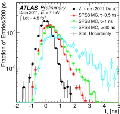
The distribution of arrival times of the photon candidates is used in the analysis as a cross check.
Figure 4 shows the timing distribution expected for selected signal events, for
Λ =120 TeV and for NLSP
lifetime values of
τ =0.5, 1 and 30 ns. The expectations for the backgrounds are determined using the
same data control samples described above. It is expected that the performance of the calorimeter timing
measurement, as determined using the second-layer cell with the maximum deposited energy, should be
rather insensitive to the details of the EM shower development. It was verified that the timing distribution
of electrons in
Z→eeevents is very similar to that of loose photon candidates in the TL control sample
with
ETmiss <20 GeV. Therefore, the timing distribution determined with the higher statistics
Z → eesample is characteristic of the timing performance expected for all prompt backgrounds, and is shown
superimposed on Figure 4.
[ns]
t
γ-2 -1 0 1 2 3 4 5
Fraction of Entries/200 ps
-210
10
-1ATLAS
Preliminary= 7 TeV s Data 2011,
Ldt = 4.8 fb-1
∫
ee (2011 Data)
→ Z
=0.5 ns SPS8 MC, τ
=1 ns τ SPS8 MC,
=30 ns τ SPS8 MC, Stat. Uncertainty
Figure 4: The distribution of photon arrival times expected for SPS8 GMSB signal models with
Λ =120 TeV and for NLSP lifetime values of
τ =0.5, 1 and 30 ns. Superimposed is the expectation for prompt backgrounds, as determined using electrons from
Z → eeevents. The uncertainties shown are statistical only.
7 Systematic Uncertainties
When fitting the photon pointing distribution in data to the templates describing the expectations from signal and background, the total number of events is normalized to the 46 events observed in the data in the signal region. In addition, the background templates are determined using data. Thus, the analysis does not rely on predictions of the background normalization or composition, and there are therefore no systematic uncertainties to consider regarding the normalization of the backgrounds. As a result, the various systematic uncertainties relevant for the analysis can be divided into two types, namely “flat”
uncertainties that are not a function of
zDCAbut that affect the overall expected signal yield, and “shape”
uncertainties related to the shapes of the unit-normalized signal and background pointing templates. The shape uncertainties, which are correlated across
zDCAbins, were discussed in Section 6; their sizes within each bin are depicted in Figure 3. The various flat systematic uncertainties are summarized in Table 2, and discussed in more detail below.
The uncertainty on the integrated luminosity is
±1.8% [40, 41]. The uncertainty on the trigger effi-
ciency is
±2.1%, which includes a contribution of
±0.5% for the determination of the diphoton trigger
efficiency using a bootstrap method [42], and a contribution of
±2% taken as a conservative estimate of
any possible dependence of the trigger efficiency on
zDCA. Uncertainties on the photon selection, the
photon energy scale, and the detailed material composition of the detector, as described in Ref. [22],
result in an uncertainty of
±4.4%. The uncertainty due to the photon isolation requirement was estimated
by varying the energy leakage and the pile-up corrections independently, resulting in an uncertainty of
Source of Uncertainty Value
Integrated Luminosity
±1.8%
Trigger Efficiency
±2.1%
Photon ID and
ETScale/Resolution
±4.4%
Photon Isolation
±1.4%
EmissT
:
ETScale/Resolution
±(1.1 – 8.2) % Signal PDF and Scale Uncertainties
±(4.7 – 6.4) % Total Systematic Uncertainty
±(7.2 – 11.7) %
Table 2: Summary of systematic uncertainties on the total signal yield. The final row provides the total of these systematic uncertainties, calculated as the quadrature sum of the various contributions. There is an additional contribution, not shown in the Table, due to MC statistics, that ranges between
±0.7% and
±
5.0%, depending mostly on the NLSP lifetime. In addition to these uncertainties on the signal yield, the analysis includes uncertainties on the shapes of the signal and background pointing templates, as depicted in Figure 3.
±
1.4%. Systematic uncertainties due to the
EmissTreconstruction, estimated by varying the cluster ener- gies and the
EmissTresolution between the measured performance and MC expectations [43], contribute an uncertainty in the range of
±(1.1
−8.2)%, with the higher uncertainty values applicable for lower values of
Λ. As described in Section 3, variations in the calculated NLO signal cross sections, timesthe signal acceptance and efficiency, at the level of
±(4.7
−6.4)% occur when varying the PDFs and factorisation and renormalisation scales. Adding these flat systematic uncertainties in quadrature gives a total systematic uncertainty on the signal yield in the range of
±(7.2
−11.7)%, to which is added a contribution in the range of
±(0.7
−5.0)% due to statistical uncertainties in the signal MC predictions.
8 Results and Interpretation
The
zDCAdistribution for the 46 loose photons of the events in the signal region with
EmissT >75 GeV is shown in Figure 5. As expected for SM backgrounds, the distribution is rather narrow, and there is no obvious sign of a significant excess in the tails that would be expected for GMSB signal photons originat- ing in the decays of long-lived neutralinos. There are three events with
|zDCA|>200 mm, including one with a value of
zDCA = +752 mm. Some additional information about these three events is summarizedin Table 3.
Run Event
EmissTLoose Photon Tight Photon
Number Number (GeV)
ET(GeV)
zDCA(mm)
tγ(ps)
ET(GeV)
zDCA(mm)
t(ps)
186721 30399675 77.1 75.9 –274 360 72.0 22 580
187552 14929851 77.3 59.4 –262 1200 87.2 –120 240
191920 14157929 77.9 56.6 752 2 54.2 5 –200
Table 3: Some relevant parameters of the three “outlier” events mentioned in the text.
The timing distribution for the 46 events in the signal region with
EmissT >75 GeV is shown in
Figure 6. The timing distribution is rather narrow, in agreement with the background-only expectation
which is shown superimposed on Figure 6, and there is no significant excess in the positive tail that
would be expected for GMSB signal photons. The photon with the largest time value has
t≈1.2 ns, and
is measured using a channel which was read out with medium gain, for which the timing resolution is
[mm]
z
DCA-1000 -800 -600 -400 -200 0 200 400 600 800 1000
Entries/Bin
0 2 4 6 8 10 12 14 16 18 20 22
Data (Signal Region)
=6 ns τ
=120 TeV, Λ
SPS8 MC,
±0.19 = 0.20 µ Best S+B Fit, Bkg Only Fit
Preliminary ATLAS
Data 2011
Ldt = 4.8 fb
-1∫
= 7 TeV, s
[mm]
zDCA
-100 -80 -60 -40 -20 0 20 40 60 80 100
Entries/Bin
0 2 4 6 8 10 12 14 16 18 20 22
Figure 5: The
zDCAdistribution for the 46 loose photons of the events in the signal region. Superimposed
are the results of the background-only fit, as well as the results of the signal-plus-background fit for the
case of
Λ =120 TeV and
τ=6 ns. The hatching shows the total uncertainties in each bin for the signal-
plus-background fit, for which the fitted signal strength is
µ=0.20
±0.19. The inlay shows an expanded
view of the central region, near
zDCA =0. The first (last) bin includes the contribution from underflows
(overflows).
≈
400 ps. This photon corresponds to one of the three events with
|zDCA| >200 mm that are discussed in Table 3, but not to the most extreme pointing outlier. For the other two events in Table 3, the timing is consistent with the hypothesis that the photon candidate is in-time.
[ns]
tγ
-3 -2 -1 0 1 2 3
Entries/200 ps
0 2 4 6 8 10 12 14 16 18
(Signal Region) Data
Bkg Only Preliminary
ATLAS Data 2011
Ldt = 4.8 fb-1
∫
s = 7 TeVFigure 6: The distribution of arrival times for the 46 loose photons of the events in the signal region.
Superimposed for comparison is the shape of the timing distribution expected for background only, nor- malized to 46 total events.
To determine the final results, the pointing distribution shown in Figure 5 is fitted using the point- ing templates described previously. The binning shown in Figure 5 is used in the fit. The background contribution is modelled in the fit as a weighted sum of the
Te/γand
TEmissT <20GeV
templates. Background-
only fits are performed to determine the compatibility of the observed pointing distribution with the background-only hypothesis. Signal-plus-background fits are performed to determine, via profile likeli- hood fits, the 95% CL limit on the signal strength,
µ, defined as the number of fitted signal events dividedby the SPS8 expectation for the signal yield. In both cases, the overall normalization is constrained to the 46 events observed in the signal region in data, and the relative weights of the two background templates is treated as a nuisance parameter in the fit.
Fit Event Range of|zDCA|values [mm]
Type Type 0−20 20−40 40−60 60−80 80−100 100−200 200−400 400−600 >600
- Data 27 7 4 1 1 3 2 0 1
Bkg Only Bkg 25.0±2.2 9.1±0.8 3.8±0.3 2.1±0.5 1.4±0.4 3.0±1.1 1.3±0.5 0.2±0.1 0.08±0.03 Signal Total 25.1±4.2 9.3±1.5 3.3±0.7 1.6±0.6 1.1±0.4 2.6±1.0 1.8±0.8 0.7±0.5 0.5±0.4
Plus Sig 0.7±0.6 0.5±0.5 0.4±0.3 0.3±0.3 0.3±0.3 1.2±1.1 1.3±1.2 0.6±0.5 0.4±0.4 Bkg Bkg 24.4±4.2 8.8±1.5 2.9±0.8 1.3±0.7 0.8±0.6 1.4±1.5 0.5±0.7 0.1±0.1 0.03±0.04
Table 4: Integrals over various
|zDCA|ranges of the distributions shown in Figure 5 for the 46 loose
photons in the signal region. The numbers of events observed in data are shown, as well as the results of
a background-only fit and a signal-plus-background fit for the case of
Λ =120 TeV and
τ=6 ns. The
fitted signal strength is
µ=0.20
±0.19. The errors shown correspond to the sum of both statistical and
systematic uncertainties. Note that the numbers of signal and background events from the signal-plus-
background fit are negatively correlated.
Table 4 shows the number of observed events in the various bins of
zDCAshown in Figure 5, except that the number of
zDCAbins is reduced for display purposes by a factor of two by taking the absolute value of
zDCA. Included in Table 4 are the results from the background-only and signal-plus-background fit, for the case of
Λ =120 TeV and
τ =6 ns. Comparing the first two rows of Table 4 shows that there is reasonable agreement between the observed data and the results of the background-only fit, though there is some excess seen in the data for larger
|zDCA|values. The
p0value for the background- only hypothesis is
≈0.060, indicating that the slight excess has a significance equivalent to
≈1.5σ. The excess is dominated by the outlier photon with
zDCA =752 mm; removing this event from the distribution and performing a new fit, one obtains a
p0value of
≈0.30, indicating in this case agreement with the background-only model.
The last three rows of Table 4 show the results of the signal-plus-background fit, including the total number of fitted events in each
|zDCA|bin, as well as the separate contributions from signal and from background. For the case of
Λ =120 TeV and
τ=6 ns, the signal-plus-background fit returns a central value for the signal strength of
µ =0.20
±0.19. The fit results are used to determine, via the CLs method [44], 95% CL limits on the number of signal events. The results, derived within the RooStats framework [45], are determined for both the observed limit, where the fit is performed to the pointing distribution of the 46 observed events in the signal region, and for the expected limit, where the fit is performed to ensembles of pseudoexperiments generated according to the background-only hypothesis.
The slight excess for larger
|zDCA|values, due largely to the photon with
zDCA =752 mm, leads to a result where the observed limit on the number of signal events is somewhat less restrictive than the expected limit. For the example of
Λ =120 TeV and
τ=6 ns, the observed (expected) 95% CL limit is 18.3 (9.8) signal events.
By repeating the statistical procedure for various
Λand
τvalues, the limits are determined as a function of these SPS8 model parameters. The top plot of Figure 7 shows the 95% CL limits on the number of signal events versus
τ, for the case withΛ =120 TeV. The bottom plot of Figure 7 shows the 95% CL limits on the allowed cross section versus
τ, also for the case withΛ =120 TeV. Each plot includes a curve indicating the SPS8 theory prediction for
Λ =120 TeV. The intersections where the limits cross the theory prediction show that, for
Λ =120 TeV, values of
τbelow 8.7 ns are excluded at 95% CL, whereas the expected limit would exclude values of
τbelow 14.6 ns.
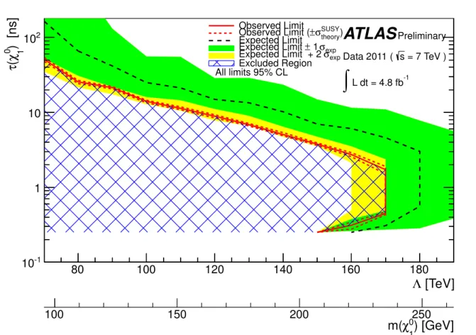
Comparing with the theoretical cross section of the SPS8 GMSB model, the results are converted into an exclusion region in the two-dimensional plane of
τversus
Λ, as shown in Figure 8. Also shownin the figure are corresponding limits on the lifetime versus mass of the lightest neutralino, where the relation between
Λand NLSP mass is taken from the theory.
9 Conclusions
A search has been performed for non-pointing photons in the diphoton plus
EmissTfinal state, using the full data sample of 7 TeV
ppcollisions recorded in 2011 with the ATLAS detector at the LHC. The analysis uses the capability of the ATLAS LAr calorimeter to measure the flight direction of photons to perform the search, with the precision measurement of the arrival time of photons used as a cross check of the results.
No significant evidence for non-pointing photons has been observed. Interpreted in the context of
the GMSB SPS8 benchmark model, the results provide 95% CL exclusion limits in the plane of
τ(the
lifetime of the lightest neutralino) versus
Λ(the effective scale of SUSY breaking) or, alternatively,
versus the mass of the lightest neutralino. For example, for
Λ =70 TeV (160 TeV), NLSP lifetimes
between 0.25 and 50.7 ns (2.7 ns) are excluded at 95% CL.
) [ns]
0
χ1
τ(
0 10 20 30 40 50 60 70 80
Signal Events
10
102 SPS8 Theory Prediction
SUSY theory
σ
± SPS8 Theory Prediction Observed Limit Expected Limit
σexp
± 1 Expected Limit
σexp
Expected Limit + 2
ATLAS
Preliminary = 7 TeV ) s Data 2011 (L dt = 4.8 fb-1
∫
= 120 TeV ΛAll limits 95% CL
) [ns]
0
χ1
τ(
0 10 20 30 40 50 60 70 80
[fb]σ
0 500 1000 1500 2000
2500 SPS8 Theory Prediction
SUSY theory
σ
± SPS8 Theory Prediction Observed Limit Expected Limit
σexp
± 1 Expected Limit
σexp
Expected Limit + 2
ATLAS
Preliminary = 7 TeV ) s Data 2011 (L dt = 4.8 fb-1
∫
= 120 TeV ΛAll limits 95% CL
Figure 7: 95% CL limits on (top) the number of signal events and (bottom) the SPS8 signal cross section,
as a function of NLSP lifetime, for the case of
Λ =120 TeV. The region below the limit curve is excluded
at 95% CL.
[TeV]
Λ
80 100 120 140 160 180
) [ns]
0 1χ ( τ
10-1
1 10 102
) [GeV]
0
χ
1100 150 200
m(
250Observed Limit
SUSY)
theory
σ
± Observed Limit ( Expected Limit
σexp
± 1 Expected Limit
σexp
Expected Limit + 2 Excluded Region
ATLAS
Preliminary = 7 TeV ) sData 2011 ( L dt = 4.8 fb-1
All limits 95% CL
∫
Figure 8: The expected and observed limits in the plane of NLSP lifetime versus
Λ(or, equivalently, versus the NLSP mass), for the SPS8 model. Linear interpolations are shown to connect between
Λvalues, separated by 10 TeV, for which MC signal samples are available. The region excluded at 95%
CL is shown as the blue hatched area. The limit is not shown below an NLSP lifetime of 0.25 ns which,
due to the MC signal samples available, is the smallest value considered in the analysis.
References
[1] H. Miyazawa, Prog. Theor. Phys.
36 (6)(1966) 1266.
[2] P. Ramond, Phys. Rev.
D3(1971) 2415.
[3] Y. A. Golfand and E. P. Likhtman, JETP Lett.
13(1971) 323.
[4] A. Neveu and J. H. Schwarz, Nucl. Phys.
B31(1971) 86.
[5] A. Neveu and J. H. Schwarz, Phys. Rev.
D4(1971) 1109.
[6] J.-L. Gervais and B. Sakita, Nucl. Phys.
B34(1971) 632.
[7] D. V. Volkov and V. P. Akulov, Phys. Lett.
B46(1973) 109.
[8] J. Wess and B. Zumino, Phys. Lett.
B49(1974) 52.
[9] J. Wess and B. Zumino, Nucl. Phys.
B70(1974) 39.
[10] P. Fayet, Phys. Lett.
B64(1976) 159.
[11] P. Fayet, Phys. Lett.
B69(1977) 489.
[12] G. R. Farrar and P. Fayet, Phys. Lett.
B76(1978) 575.
[13] P. Fayet, Phys. Lett.
B84(1979) 416.
[14] S. Dimopoulos and H. Georgi, Nucl. Phys.
B193(1981) 150.
[15] M. Dine and W. Fischler, Phys. Lett.
B110(1982) 227.
[16] L. Alvarez-Gaum,M. Claudson, and M. B. Wise, Nucl. Phys.
B207(1982) 96.
[17] C. R. Nappi and B. A. Ovrut, Phys. Lett.
B113(1982) 175.
[18] M. Dine and A. Nelson, Phys. Rev.
D48(1993) 1277,
hep-ph/9303230.[19] M. Dine, A. Nelson, and Y. Shirman, Phys. Rev.
D51(1995) 1362,
hep-ph/9408384.[20] M. Dine, A. Nelson, Y.Nir, and Y. Shirman, Phys. Rev.
D53(1996) 2658,
hep-ph/9507378.[21] B. C. Allanach et al., Eur. Phys. J.
C25(2002) 113,
hep-ph/0202233.[22] ATLAS Collaboration, Phys. Lett.
B718(2012) 411,
arXiv:1209.0753 [hep-ex].[23] CMS Collaboration,
arXiv:1212.1838 [hep-ex].[24] ATLAS Collaboration, JINST
3(2008) S08003.
[25] ATLAS Collaboration, Phys. Lett.
B716(2012) 1,
arXiv:1207.7214 [hep-ex].[26] N. Buchanan et al., JINST
3(2008) P03004.
[27] H. Abreu et al., JINST
5(2010) P09003.
[28] M. Aharrouche et al., Nucl. Instrum. Meth.
A597(2008) 178.
[29] F. E. Paige, S. D. Protopopescu, H. Baer, and X. Tata,
hep-ph/0312045.[30] W. Beenakker, R. Hopker, and M. Spira,
hep-ph/9611232.[31] P. M. Nadolsky et al., Phys. Rev.
D78(2008) 013004,
arXiv:0802.0007 [hep-ph].[32] M. Kramer et al.,
arXiv:1206.2892 [hep-ph].[33] M. Bahr et al., Eur. Phys. J.
C58(2008) 639,
arXiv:0803.0883 [hep-ph].[34] A. Sherstnev and R. S. Thorne, Eur. Phys. J.
C55(2008) 553,
arXiv:0711.2473 [hep-ph].[35] ATLAS Collaboration, Eur. Phys. J.
C70(2010) 823,
arXiv:1005.4568 [physics.ins-det].[36] GEANT4 Collaboration, S. Agostinelli et al., Nucl. Instrum. Meth.
A506(2003) 250.
[37] ATLAS Collaboration, Phys. Rev. D
83, 052005 (2011), arXiv:1012.4389 [hep-ex].[38] ATLAS Collaboration, Eur. Phys. J.
C72(2012) 1909,
arXiv:1110.3174 [hep-ex].[39] ATLAS Collaboration, Phys. Lett. B
710(2012) 519, arXiv:1111.4116 [hep-ex].
[40] ATLAS Collaboration, Eur. Phys. J. C
71, 1630 (2011), arXiv:1101.2185 [hep-ex].[41] ATLAS Collaboration, ATLAS-CONF-2011-116, 2011.
http://cdsweb.cern.ch/record/1367408.
[42] ATLAS Collaboration, Eur. Phys. J.
C72(2012) 1849,
arXiv:1110.1530 [hep-ex].[43] ATLAS Collaboration, Eur. Phys. J.
C72(2012) 1844,
arXiv:1108.5602 [hep-ex].[44] A. L. Read, J. Phys.
G28(2002) 2693.
[45] L. Moneta et al., PoS
ACAT2010(2010) 057,
arXiv:1009.1003 [physics.data-an].Supplemental Plots
[mm]
z
DCA-1000 -800 -600 -400 -200 0 200 400 600 800 1000
Entries/Bin
0 2 4 6 8 10 12 14 16 18 20 22
Data (Signal Region)
Bkg Only Fit
Preliminary ATLAS
Data 2011
Ldt = 4.8 fb
-1∫
= 7 TeV, s
[mm]
zDCA
-100 -80 -60 -40 -20 0 20 40 60 80 100
Entries/Bin
0 2 4 6 8 10 12 14 16 18 20 22
Figure 9: The
zDCAdistribution for the 46 loose photons of the events in the signal region. Superimposed
are the results of the background-only fit. The hatching shows the total uncertainties in each bin for the
signal-plus-background fit. The inlay shows an expanded view of the central region, near
zDCA =0.
[mm]
z
DCA-1000 -800 -600 -400 -200 0 200 400 600 800 1000
Entries/Bin
0 2 4 6 8 10 12 14 16 18 20 22
Data (Signal Region)
=6 ns τ
=120 TeV, Λ
SPS8 MC,
±0.19 = 0.20 µ Best S+B Fit,
Bkg component in Sig+Bkg Fit
Preliminary ATLAS
Data 2011
Ldt = 4.8 fb
-1∫
= 7 TeV, s
[mm]
zDCA
-100 -80 -60 -40 -20 0 20 40 60 80 100
Entries/Bin
0 2 4 6 8 10 12 14 16 18 20 22