ATLAS-CONF-2012-087 07July2012
ATLAS NOTE
ATLAS-CONF-2012-087
July 2, 2012
Search for Extra Dimensions in the Diphoton Channel using 4 . 9 fb
−1of Proton-Proton Collisions recorded at √
s = 7 TeV with the ATLAS Detector
The ATLAS Collaboration
Abstract
The large difference between the Planck scale and the electroweak scale, known as the hierarchy problem, is addressed in certain models through the postulate of extra spatial di- mensions. We perform a search for evidence of extra spatial dimensions in the diphoton channel using the full set of proton-proton collisions at
√s =
7 TeV recorded in 2011 with the ATLAS detector at the CERN Large Hadron Collider. This dataset corresponds to an integrated luminosity of 4.9 fb
−1. The diphoton invariant mass spectrum is observed to be in good agreement with the expected Standard Model background. We set 95 % CL lower limits of between 2.62 and 3.92 TeV on the
MSscale in the context of the model proposed by Arkani-Hamed, Dimopoulos, Dvali (ADD), depending on the number of extra dimensions and the theoretical formalism used. In the context of the Randall-Sundrum (RS) model, a lower limit of 1.00 (2.06) TeV at 95 % CL is set on the mass of the lightest RS graviton for RS couplings of
k/MPl=0.01 (0.1).
c Copyright 2012 CERN for the benefit of the ATLAS Collaboration.
Reproduction of this article or parts of it is allowed as specified in the CC-BY-3.0 license.
1 Introduction
One of the major goals of particle physicists in the past decades has been to solve the hierarchy problem:
the fact that the electroweak scale is 16 orders of magnitude smaller than the Planck mass scale. One possible solution to the hierarchy problem is the existence of extra spatial dimensions.
In the Randall-Sundrum (RS) model [1], a five-dimensional geometry is assumed, in which the fifth dimension is compactified with length
rc. There are two four-dimensional branes sitting in a five- dimensional bulk with a “warped” geometry. The Standard Model (SM) fields are located on the so- called TeV brane, while gravity originates from the other brane, called the Planck brane. Gravitons are capable of propagating in the bulk. Mass scales on the TeV brane - such as the Planck mass (M
Pl) de- scribing the observed strength of gravity - correspond to mass scales on the Planck brane (M
D) as given by
MD = MPle−kπrc, where
kis the curvature scale of the extra dimension. The observed hierarchy of scales can be naturally reproduced in this model, if
krc ≈12 [2]. The compactification of the extra dimension gives rise to a Kaluza-Klein (KK) tower of graviton excitations
G, an infinite set of particleswith increasing masses, located on the TeV brane. The phenomenology can be described in terms of the mass of the lightest KK graviton excitation (m
G) and the dimensionless coupling to the SM fields,
k/MPl, where
MPl = MPl/√8π is the reduced Planck scale. From theoretical arguments [2],
k/MPlis preferred to have values in the range [0.01, 0.1]. The lightest RS graviton is expected to be a fairly narrow resonance up to
k/MPl<0.3. The most stringent experimental limits on RS gravitons have been obtained at the LHC: the 95 % confidence level (CL) lower limits on the graviton mass for
k/MPl=0.1 are 1.95 TeV [3] from an analysis combining the
G → ee/µµchannels with 1.1 fb
−1and the
G → γγchannel with 2.1 fb
−1of data collected by the ATLAS experiment, and 1.84 TeV with 2.2 fb
−1from the CMS experiment [4] in the
G → γγchannel. The limits from earlier searches at the Tevatron can be found in Ref. [5].
Arkani-Hamed, Dimopoulos, and Dvali (ADD) [6] proposed a different scenario for extra dimen- sions. Motivated by the weakness of gravity, they postulated the existence of
nflat additional spatial dimensions compactified with radius
R, and proposed a model in which only gravity propagates in theextra dimensions. The fundamental Planck scale in the (4
+n)-dimensional spacetime,MD, is related to the apparent scale
MPlby Gauss’ law:
M2Pl = Mn+2D Rn. The mass splitting of the graviton KK modes is 1/R for each of the
nextra dimensions. In the ADD model, resolving the hierarchy problem usually requires small values of 1/R, giving rise to an almost continuous spectrum of KK graviton states. We use the symbol
Gto denote KK graviton states in both the RS and ADD models. The existence of ADD extra dimensions can manifest itself in proton-proton (pp) collisions through a variety of processes, in- cluding virtual graviton exchange as well as direct graviton production. While processes involving direct graviton emission depend on
MD, effects involving virtual gravitons depend on the ultraviolet cutoff of the KK spectrum, denoted
MS. The strength of gravity in the presence of extra dimensions is typ- ically parameterised by
ηG = F/MS4, where
Fis a dimensionless parameter of order unity reflecting the dependence of virtual KK graviton exchange on the number of extra dimensions. Several theoretical formalisms exist in the literature, using different definitions of
Fand, consequently, of
MS:
F =
1, (GRW) [7]; (1)
F =
log
M2 S
ˆ s
n=
2
2
n−2 n>
2
,
(HLZ) [8]; (2)
F =±
2
π,
(Hewett) [9]; (3)
where
√ˆ
s
is the centre-of-mass energy of the parton-parton collision. The effect of ADD graviton ex- change manifests itself as a non-resonant deviation from the SM background expectation. The effective diphoton cross section is the result of the SM and ADD amplitudes, as well as their interference. The interference term in the effective cross section is linear in
ηGand the pure graviton exchange term is quadratic in
ηG. In previous analyses by the ATLAS and CMS collaborations, 95 % CL lower limits on
MSbetween 2.26 and 3.52 TeV [3] and 2.3 to 3.8 TeV [4] were set depending on the theoretical formal- ism used. Searches for ADD virtual graviton effects have also been performed at other colliders,
e.g.at HERA [10], LEP [11] and the Tevatron [12].
In this Note, we report the results of a search for extra dimensions in the diphoton channel using the full data sample recorded by the ATLAS detector in 2011, corresponding to a total integrated luminosity of 4.9 fb
−1of
√s=
7 TeV
ppcollisions. The results are interpreted in the context of both the ADD and RS scenarios. The diphoton channel is particularly sensitive for this search due to the clean experimental signature, excellent mass resolution and modest backgrounds. The branching ratio for graviton decay to two photons is twice the value of that for graviton decay to any individual charged-lepton pair. This search is an extension of an earlier study [3] performed with 2.1 fb
−1. Many of the techniques developed in Ref. [3] are reused in the present study. Refinements in the background estimate are described in detail below. The dataset from Ref. [3] is included in the present study. It has been reprocessed in order to benefit from improvements in the reconstruction and calibration procedures.
2 The ATLAS Detector
The ATLAS detector is a multipurpose particle physics instrument with a forward-backward symmetric cylindrical geometry and near 4π solid angle coverage.
1A detailed description of the ATLAS detector can be found in Ref. [13]. The inner tracking detector (ID) consists of a silicon pixel detector, a sili- con microstrip detector, and a transition radiation tracker. The ID is surrounded by a superconducting solenoid that provides a 2 T magnetic field. The ID allows an accurate reconstruction of tracks from the primary
ppcollision and also identifies tracks from secondary vertices, permitting the efficient recon- struction of photon conversions in the ID, which is particularly important for this analysis.
The electromagnetic calorimeter (ECAL) is a lead/liquid-argon (LAr) sampling calorimeter with an accordion geometry. It is divided into a barrel section, covering the pseudorapidity
2region
|η| <1.475, and two endcap sections, covering the pseudorapidity regions 1.375
< |η| <3.2. It consists of three longitudinal layers. The first one uses highly granular “strips” segmented in the
ηdirection for efficient event-by-event discrimination between single photon showers and two overlapping showers originating from
π0decay. The second layer of the electromagnetic calorimeter collects most of the energy deposited in the calorimeter by photon showers. Significant energy deposits in the third layer are an indication for leakage beyond the ECAL from a high energy shower. The measurements from the third layer are used to correct for this effect. A thin presampler layer in front of the accordion calorimeter, covering the pseudorapidity interval
|η|<1.8, is used to correct for energy loss upstream of the calorimeter.
The hadronic calorimeter (HCAL), surrounding the ECAL, includes a central (
|η|<1.7) iron/scintillator tile calorimeter, two end-cap (1.5
< |η| <3.2) copper/LAr calorimeters and two tungsten/LAr forward calorimeters that extend the coverage to
|η|<4.9. The muon spectrometer, located beyond the calorime- ters, consists of three large air-core superconducting toroid systems, instrumented with precision tracking chambers as well as fast detectors for triggering.
1The right-handed coordinate system of the detector is defined such that the origin is at the nominal interaction point. The beam direction defines the z-axis and the x - y plane is transverse to the beam. The positive x-axis points from the interaction point to the centre of the LHC ring and the positive y-axis points upwards. The azimuthal angleφis measured around the beam axis and the polar angleθis the angle from the beam axis.
2The pseudorapidityηis defined in terms of the polar angleθbyη=−ln tan(θ/2).
3 Trigger and Event Selection
The analysis uses data recorded by ATLAS between March and October 2011 during stable beam periods of 7 TeV
ppcollisions. A three-level trigger system is used to select events containing two photon candidates. The first level trigger is hardware-based and relies on a readout with coarse granularity. The second and third level triggers, collectively referred to as the high-level trigger (HLT), are implemented in software and exploit the full granularity and energy calibration of the calorimeter. Selected events have to satisfy a diphoton trigger where each photon is required to satisfy, at the HLT level, a transverse energy requirement
EγT>20 GeV and a set of requirements [14] on the shape of the energy deposit. This set includes criteria on the energy leakage in the hadronic calorimeter and on the width of the shower in the second layer of the ECAL. This trigger is nearly 100 % efficient for diphoton events passing the final selection requirements.
Only events satisfying the standard ATLAS data quality requirements and having at least one primary collision vertex with at least three tracks are kept. Photon candidates reconstructed in the precision regions of the barrel (
|η|<1.37) or the end-caps (1.52
<|η|<2.37), with
EγT>25 GeV and satisfying the same requirements on the shower shape as the trigger are preselected. These requirements on the photon candidates are referred to as loose selection. The two highest-E
γTphoton candidates each have to satisfy a set of stricter requirements, referred to as the tight photon definition [14], which includes a more stringent selection on the shower width in the second layer of the ECAL and additional requirements on the energy distribution in the first layer of the ECAL. In addition, the two photon candidates of interest have to satisfy a calorimetric isolation requirement,
ETiso <5 GeV. This isolation is computed by summing the transverse energy over the cells of the calorimeters in a cone of radius
∆R= p(η
−ηγ)
2+(φ
−φγ)
2<0.4 surrounding the photon candidate. Here (η, φ) denotes the cell position and (η
γ, φγ) denotes the position of the photon cluster. The transverse energy contribution in the centre of the cone - which contains the photon cluster - is subtracted, and corrections are applied to account for the expected energy leakage from the photon into the isolation region. An ambient energy correction, based on the measurement of low- transverse-momentum jets [15] is also applied, on an event-by-event basis, to remove the contributions from the underlying event and from pileup, which results from the presence of multiple
ppcollisions within the same or nearby bunch crossings. Finally a total of 15135 events with a diphoton invariant mass greater than 142 GeV are selected
3.
4 Event Simulation
We use Monte Carlo (MC) simulations to study the response of the detector to various RS and ADD scenarios as well as SM diphoton processes. The MC generators that we use are listed below. For samples generated using P
ythia[16], the ATLAS parameter tunes [17] are used in the event generation.
For samples generated using P
ythiaor S
herpa[18], the generated events are processed through the G
eant4 [19] detector simulation. Then the simulated events are reconstructed with the same procedure as used for the data. To reproduce the pileup conditions of the data, the simulated events are reweighted to match the data in terms of the distribution of the number of interactions per bunch crossing. The determination of the number of interactions per bunch crossing is discussed in Ref. [20].
P
ythia6.424 with MRST2007LOMOD [21] parton distribution functions (PDFs) is used to simulate the SM diphoton production at LO. In addition, the NLO correction and the contribution of the fragmen- tation processes are evaluated using D
iphox[22] 1.3.2 with MSTW2008NLO [23] PDFs and lead to an invariant-mass-dependent correction of the P
ythiaprediction. To apply this correction, the events sim- ulated using P
ythiaand the G
eant4-based detector simulation are reweighted, at the generator level, to
3The exact value (142 GeV) for the requirement on the invariant mass has been chosen to coincide with the lower edge of the first bin in Fig. 1.
the invariant mass spectrum predicted using D
iphox. Samples of RS events are produced using the same generator and PDFs as for the SM diphoton samples. They are used to study the selection efficiency and the shape of the reconstructed invariant mass spectrum for various values of the graviton mass
mGbe- tween 400 GeV and 3000 GeV and values of
k/MPlin the range [0.01, 0.1]. ADD models are simulated for various
MSvalues using S
herpa1.2.3 with CTEQ6L [24] PDFs. The ADD MC samples are used to evaluate the number of signal events passing the selection as a function of
MS. We also consider an NLO K-factor of 1.75
±0.10 for the RS scenario and of 1.70
±0.10 for the ADD scenario. These K-factors have been provided by the authors of Refs. [25, 26].
5 Background Estimate
The dominant background in this analysis is the irreducible background due to SM
γγproduction. An- other significant background component is the reducible background which arises from events in which one or both of the photon candidates result from a different object being misidentified as a photon. This background is dominated by
γ+jet (
j) andj+jevents, with one or two jets faking photons, respectively.
Backgrounds with electrons faking photons, such as the Drell-Yan production of electron-positron pairs as well as
W/Z + γand
ttprocesses, have been verified to be small after the event selection and are neglected.
We first describe the tools and samples that are used to predict the contributions from the SM
γγbackground and from the reducible background to the high-mass signal region, as well as their main limitation. We then describe in detail the two-step procedure that is used to overcome this limitation and to obtain our background estimate.
In our estimate of the irreducible background, we make use of the NLO calculations [22] that are available for the SM
γγproduction processes. The uncertainty in the absolute normalisation of the
γγcross section is, however, quite substantial:
≃20 % (
≃25 %) uncertainty on the cross section for
γγevents with an invariant mass
mγγ >200 GeV (m
γγ >1200 GeV) with both photons in the detector acceptance. We therefore normalise our background estimates, which are discussed in detail below, to the data in the low-mass control region
4([142, 409] GeV) where the presence of any signal has been excluded by previous searches. Compared to the use of NLO calculations to predict the absolute rate of SM
γγproduction in the high-mass signal region, the use of NLO calculations for the extrapolation of the SM
γγproduction rates from the low-mass control region to the high-mass signal region results in significantly smaller uncertainties. The extrapolation method is described in detail below, along with quantitative estimates of the final uncertainties.
The reducible background is estimated using data-driven techniques. We split the reducible back- ground into three components:
γ+ jevents (the leading-E
Tphoton candidate is due to a real photon),
j+γ(fake leading photon candidate) and
j+ j. Separately for each component, we define several datacontrol samples that are enriched in the given component.
Following these considerations, we proceed in two steps to estimate the
mγγspectrum of the back- ground events. We first determine the shape of the
mγγspectrum, separately for each of the four back- ground components. We then determine the normalisation for each component using the low-mass con- trol region. The shape of the
mγγspectrum from SM
γγproduction is estimated using simulated events, reweighting the P
ythiasamples to the differential (in
mγγ) cross section predicted using D
iphox. The shape of the
γ+ jbackground is estimated from a data control sample that is selected in the same way as the signal sample, except that the subleading
γcandidate is required to pass loose identification criteria and to fail tight identification criteria. The control samples used to extract the shapes of the
mγγspectra of
j+γand
j+ jbackgrounds are defined following the same approach,
i.e.by requiring the leading
4The exact values of the upper and lower bound of the low-mass control region have been chosen to coincide with the boundaries of the first bin in Table 1.
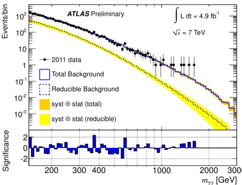
Events/bin
10-3
10-2
10-1
1 10 102
103
2011 data Total Background Reducible Background
stat (total)
⊕ syst
stat (reducible)
⊕ syst
= 1.5 TeV mG
= 0.1, MPl
RS, k/
= 2.5 TeV MS
ADD, GRW,
Preliminary
ATLAS -1
L dt = 4.9 fb
∫
s = 7 TeV[GeV]
γ
mγ
200 300 400 1000 2000 3000
Significance
-2 0 2
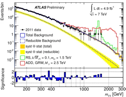
Figure 1: (Upper) Observed invariant mass distribution of diphoton events. Superimposed are the SM background expectation and the expected signals for two examples of RS and ADD models. In addition to the total background, the contribution from the reducible component is shown. To compensate the rapid decrease of the spectrum, the bins have been chosen to have constant logarithmic width. Specifically, the ratio of the upper and lower bin boundary is equal to 1.038 for all bins, and the first bin starts at 142 GeV.
(Lower) Bin-by-bin significance of the difference between data and predicted background.
photon candidate (
j+γbackground) or both candidates (
j+ jbackground) to pass loose and to fail tight identification criteria. Since the data control samples contain relatively few events at high
mγγ, a fit to a smooth function of the form
f(m
γγ)
= p1×mγγ
p2+p3logmγγ
, where the
piare free parameters, is used to extrapolate the reducible background shapes to higher masses. This functional form has been used in previous ATLAS searches in the dilepton [27], dijet [28] and diphoton [3] channels, and it describes well the shapes of the data control samples. In contrast to the earlier version of this analysis [3], the shapes of the three components of the reducible background are modelled separately.
To determine the contributions of each of the four background components to the low-mass control region, a two-dimensional template fit to the distributions of the calorimetric isolation (E
Tiso) of the two photon candidates is used. For the purpose of this fit, the isolation requirement in the event selection is relaxed to
ETiso <25 GeV. This method has been used previously in Refs. [29, 30] and in an earlier version of this analysis [3]. Templates for the
EisoTdistribution of true photons and of fake photons from jets are both determined from data. The shape for fake photons is determined using a sample of photon candidates that pass loose identification requirements and fail the tight requirements. The shape for photons is found from the sample of tight photon candidates, after subtracting the fake photon shape normalised to match the number of candidates with large values of
EisoT(specifically
EisoT >10 GeV; this control region is dominated by fake photons). Both signal and fake templates are constructed separately for leading and subleading photon candidates. The significant correlation (
∼20 %) between the
EisoTvalues of the two fake photons in the
j+ jbackground are included in the two-dimensional template for this background component.
The background expectation as a function of
mγγis summarised in Fig. 1 and Table 1. Figure 2
details the different contributions to the uncertainty in the background expectation. The uncertainties in
Mass Window Background Expectation Observed
(GeV) Irreducible Reducible Total Events
[142, 409] 10195
±1100 4586
±1100 14781 14781
[409, 512] 192
±26 43
±10 235
±20 221
[512, 596] 57
±8 10.7
±2.7 68
±7 62
[596, 719] 35
±5 5.4
±1.5 40
±4 38
[719, 805] 12.0
±1.8 1.4
±0.4 13.3
±1.6 13 [805, 901] 7.8
±1.2 0.70
±0.23 8.5
±1.1 10 [901, 1008] 4.6
±0.7 0.35
±0.13 5.0
±0.7 2 [1008, 1129] 2.7
±0.4 0.18
±0.07 2.8
±0.4 2 [1129, 1217] 1.14
±0.18 0.064
±0.028 1.21
±0.18 2 [1217, 1312] 0.72
±0.12 0.040
±0.018 0.76
±0.11 0 [1312, 1414] 0.50
±0.08 0.024
±0.012 0.53
±0.08 2 [1414, 1525] 0.36
±0.06 0.015
±0.008 0.37
±0.06 1 [1525, 2889] 0.64
±0.12 0.022
±0.014 0.66
±0.12 1
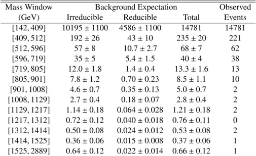
Table 1: Expected numbers of events from the irreducible and reducible background components, as well as the total background prediction and observed numbers of events in each bin of
mγγ. The boundaries of all bins in this table have been chosen to coincide with bin boundaries in Fig. 1. As discussed in the text, the background estimate is normalised to the data in the low-mass control region [142, 409] GeV. Since the uncertainties in the normalisation are strongly anticorrelated between the reducible and irreducible components, their impact on the estimate of the total background is smaller than their impact on the individual components.
the shape of the irreducible background are dominated by the uncertainties in the PDFs that are used with D
iphox. Those uncertainties are evaluated using the MSTW2008 NLO eigenvector PDF sets and using CTEQ6.6 and MRST2007LOMOD PDF sets for comparisons. The spread of the variations includes the difference between the central values obtained with the different PDF sets. Smaller contributions arise from residual imperfections in the simulation of the isolation variable
EisoTand from higher-order contributions that are not included in the D
iphoxmodel. The shape predictions from D
iphoxare found to be in good agreement with those obtained using an alternative NLO generator, MCFM [31] (with the same PDF set as D
iphox). The small difference between the two generators is assigned as an additional systematic uncertainty. It represents a negligible contribution for
mγγ >1 TeV. The uncertainties in the shape of the reducible background arise from finite statistics in the background control samples, and from the extrapolation of the background shapes from the control sample to the signal region. The latter are assessed by varying the definition of the loose selection requirement which is used to define the control samples. The impact of the shape of the reducible background on the total background is limited (Fig. 2) mainly because the reducible background is a small contribution to the total (Table 1).
The uncertainties in the normalisation of the background components are dominated by the uncertainties in the templates used in the fit to the
EisoTdistributions. The uncertainties in the templates are assessed by varying the definition of the loose selection requirement used in the extraction of the templates. They are then propagated to the normalisations by repeating the template fits with the varied templates.
6 Systematic Uncertainties in the Signal Models
Experimental systematic uncertainties on the signal yields are evaluated for both RS and ADD signals.
The systematic uncertainties are dominated by an uncertainty of
∼8 % (with a weak dependence on
[GeV]
γ
mγ
500 1000 1500 2000 2500 3000
Uncertainty as Fraction of the Total Background
0 0.05 0.1 0.15 0.2 0.25 0.3 0.35
Total uncertainty Irreducible background Yields estimate Reducible background
Preliminary ATLAS
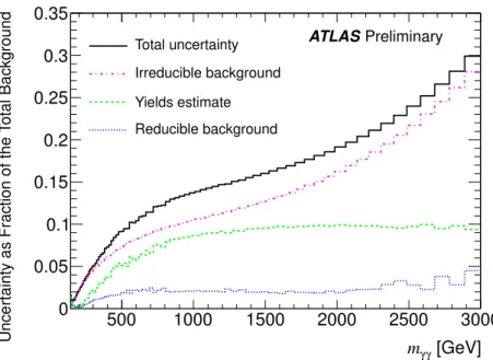
Figure 2: Uncertainty in the total background expectation as a function of
mγγ. Also shown are the individual contributions from the uncertainties in the shapes of the irreducible and the reducible com- ponents, as well as the contribution from the uncertainties in the yields (normalisations) of the different background components extracted from the low-mass control region.
the signal scenario) to cover disagreements between data and simulation in the variables used for the identification and isolation of the photons. The uncertainty on the integrated luminosity is 3.9 % [32].
An uncertainty of 2 % on the trigger efficiency arises from differences between the measured trigger efficiency in data and simulated samples. Given that the sum in quadrature of all experimental systematic uncertainties depends only weakly on the signal scenario, one common number is used in the following for all scenarios: a 9.1 % relative uncertainty on the signal yield.
Uncertainties from limited statistics in the MC samples, as well as uncertainties in the RS resonant shape due to the current knowledge of the EM energy scale, the resolution of the detector and the pileup conditions were verified to be negligible.
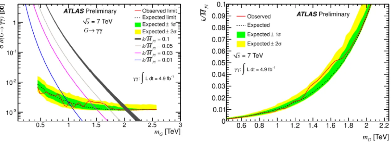
The theoretical uncertainties considered in this analysis are detailed in Ref. [3]. To summarise, an uncertainty of 10 % to 15 % in the signal yields due to PDFs is considered for ADD, 5 % to 10 % for RS. The theory uncertainties are not included in the limit calculation, but their size is presented in Fig. 3, where the graphical representations of limits discussed in Section 7 are shown.
7 Results and Interpretation
A comparison of the observed invariant mass spectrum of diphoton events and the background expecta-
tion is shown in Fig. 1, along with the statistical significance of the bin-by-bin difference [33] between
data and the expected background. This significance is plotted as positive (negative) for bins with an
excess (deficit) of data. Also shown are the expected signals for two examples of RS and ADD mod-
els. Both Fig. 1 and Table 1 show that, over the entire
mγγrange, the data are in good agreement with
the expectations from SM backgrounds. We use the B
umpH
unteralgorithm [34] to further quantify
the level of agreement between data and the SM background expectation. The B
umpH
unterperforms
a scan of the mass spectrum in windows of progressively increasing width. It identifies the window
[TeV]
mG
0.5 1 1.5 2 2.5 3
[pb])γγ→ B(Gσ
10-3
10-2
10-1
1
Observed limit Expected limit σ
± 1 Expected
σ
± 2 Expected
= 0.1 MPl
k/
= 0.05 MPl
k/
= 0.03 MPl
k/
= 0.01 MPl
k/
Preliminary ATLAS
γ γ
→ G
= 7 TeV s
L dt = 4.9 fb-1
∫
γ: γ
[TeV]
mG
0.6 0.8 1 1.2 1.4 1.6 1.8 2 2.2
PlMk/
0 0.01 0.02 0.03 0.04 0.05 0.06 0.07 0.08 0.09 0.1
Observed Expected
σ
± 1 Expected
σ
± 2 Expected
Preliminary ATLAS
= 7 TeV s
L dt = 4.9 fb-1
∫
γ: γ
Figure 3: (Left) Expected and observed 95 % CL limits on
σB, the product of the RS graviton productioncross section and the branching ratio for graviton decay via
G→γγ, as a function of the graviton mass.The theory curves are obtained using the P
ythiagenerator, which implements the calculations from Ref. [36]. A K-factor of 1.75 is applied on top of these predictions to account for NLO corrections. The thickness of the theory curve for
k/MPl =0.1 illustrates the theoretical uncertainties. (Right) The RS results interpreted in the plane of
k/MPlversus graviton mass. The region above the curve is excluded at 95 % CL.
with the most significant excess of data events over the background expectation. In this analysis, the mass spectrum is scanned from 142 to 3000 GeV. The most significant excess is found in the region 1312
<mγγ <1644 GeV. The probability to observe, due to fluctuations in the background only, an ex- cess that is at least as significant as the one in data is 0.86, which confirms the good agreement between the data and the background expectation.
Given the absence of evidence for a signal, we determine 95 % CL upper limits on the RS signal cross section. The limits are computed using a Bayesian approach [35] assuming a flat prior on the RS cross section. The likelihood function is defined as the product of the Poisson probabilities over all mass bins in the search region defined as
mγγ >409 GeV. In each bin the Poisson probability is evaluated for the observed number of data events given the model prediction. The model prediction is the sum of the expected background and the expected signal yield. The expected signal yield is a function of the graviton mass
mGand the signal cross section times branching fraction
σB(G → γγ). The resultinglimits are shown in the left part of Fig. 3. The limit can be interpreted in the plane (m
G,k/MPl) using the theoretical dependence of the cross section on these parameters (right part of Fig. 3). Alternatively, for a given value of
k/MPl, the limit can be translated into a limit on
mG. The limits on
mGare summarised in Table 2. Using a constant K-factor of 1.75, the 95 % CL lower limit is
mG>1.00 (2.06) TeV for
k/MPl=0.01 (0.1).
We perform a counting experiment to set limits on the ADD model. Specifically, we count the
number of diphoton events in a search region above a given threshold in
mγγ. The mass threshold is
chosen to optimise the expected limit on the difference in the diphoton cross section for
mγγ>500 GeV
between the ADD model and the SM-only hypothesis. For the purpose of this optimisation, a specific
implementation of the ADD model and specific values of the parameters have to be chosen. For
n =2,
MS =2500 GeV in the GRW convention, we obtain an optimal search region at
mγγ>1217 GeV. In the
data, 4 events are observed in the search region, with a background expectation of 2.32
±0.37 events. The
expected and observed 95 % CL upper limits on the number of signal events above the SM background
in the search region are given in Table 3. These limits on the event yield can be translated into limits on
K-factor value
95 % CL Observed (Expected) Limit [TeV]
k/MPl
value
0.01 0.03 0.05 0.1
1 0.87 (0.88) 1.31 (1.36) 1.49 (1.60) 1.91 (1.92) 1.75 1.00 (0.98) 1.37 (1.49) 1.63 (1.73) 2.06 (2.05)
Table 2: 95 % CL lower limits on the mass [TeV] of the lightest RS graviton, for various values of
k/MPl. The results are shown for both LO (K-factor
=1) and NLO (K-factor
=1.75) theory cross section calculations.
Expected limit Observed limit
−
2σ
−1σ mean
+1σ +2σ3.08 3.08 5.18 5.96 8.53 7.21
Table 3: Expected and observed limits at 95 % CL on the number of signal events in the search region at
mγγ>1217 GeV.
the parameter
ηGof the ADD model using a prediction of the expected excess of events over the SM-only
background as a function of
ηG. This translation is shown, for one specific implementation of the ADD
model, in Fig. 4. The limits for different ADD scenarios are summarised in Table 4. Using a constant
K-factor of 1.70, the 95 % CL upper (lower) limit on
ηGis 0.0085 (
−0.0159) TeV
−4for constructive
(destructive) interference.
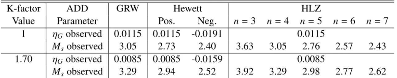
K-factor ADD GRW Hewett HLZ
Value Parameter Pos. Neg.
n=3
n=4
n=5
n=6
n=7
1
ηGobserved 0.0115 0.0115 -0.0191 0.0115
Ms
observed 3.05 2.73 2.40 3.63 3.05 2.76 2.57 2.43
1.70
ηGobserved 0.0085 0.0085 -0.0159 0.0085
Ms
observed 3.29 2.94 2.52 3.92 3.29 2.98 2.77 2.62 Table 4: 95 % CL limits on the ADD model parameters
ηGhTeV
−4iand
MS[TeV] for the various ADD models.
-4] [TeV ηG
-0.04 -0.02 0 0.02 0.04
Number of signal events
0 10 20 30 40 50 60 70 80
Preliminary ATLAS
L dt = 4.9 fb-1
∫
γ: γ
= 7 TeV s
= -0.0191
ηG = 0.0115
ηG
MonteCarlo predictions Observed limit Expected limit σ
± 1 Expected
σ
± 2 Expected
Figure 4: Number of signal events as a function of
ηG. The red horizontal line corresponds to the observed limit, the dashed line corresponds to the expected limit and the green (resp. yellow) band to the
±1σ (
±2σ) uncertainty on the expected limit. The black points correspond to MC predictions from various ADD samples without applying the K-factor of 1.70. The samples at positive (negative)
ηGhave been simulated using the GRW (Hewett) formalism. The black line is an interpolation of those predictions. When the prediction is greater than the limit line, the corresponding value for
ηGis excluded.
8 Summary
We present a search for evidence of extra dimensions in the diphoton channel, based on the full 2011 dataset collected by the ATLAS detector (4.9 fb
−1recorded at
√s =
7 TeV). A lower limit of 1.00 (2.06) TeV at 95 % CL is set on the mass of the lightest RS graviton, for RS couplings of
k/MPl =0.01 (0.1). In the ADD scenario, lower limits of between 2.62 and 3.92 TeV at 95 % CL are set on the
MSscale, depending on the number of extra dimensions and the theoretical formalism used.
9 Acknowledgements
We thank M. C. Kumar, P. Mathews, V. Ravindran and A. Tripathi for the calculation of NLO K-factors
used in this Letter.
References
[1] L. Randall and R. Sundrum, Phys. Rev. Lett.
83, 3370 (1999).[2] H. Davoudiasl, J. L. Hewett, and T. G. Rizzo, Phys. Rev. Lett.
84, 2080 (2000).[3] ATLAS Collaboration, Phys. Lett.
B710, 538 (2012).[4] CMS Collaboration, arXiv:1112.0688 [hep-ex] (2011).
[5] D0 Collaboration, Phys. Rev. Lett.
104, 241802 (2010); CDF Collaboration, Phys. Rev. Lett.107,051801 (2011).
[6] N. Arkani-Hamed, S. Dimopoulos, and G. R. Dvali, Phys. Lett.
B429, 263 (1998).[7] G. Giudice, R. Rattazzi, and J. Wells, Nucl. Phys.
B544, 3 (1999).[8] T. Han, J. Lykken, and R.-J. Zhang, Phys. Rev.
D59, 105006 (1999).[9] J. Hewett, Phys. Rev. Lett.
82, 4765 (1999).[10] H1 Collaboration, Phys. Lett.
B568, 35 (2003); ZEUS Collaboration, Phys. Lett.B591, 23 (2004).[11] LEP Working Group LEP2FF/02-02 (2002); LEP Working Group LEP2FF/03-01 (2003); ALEPH Collaboration, Eur. Phys. J.
C49, 411 (2007).[12] D0 Collaboration, Phys. Rev. Lett.
102, 051601 (2009); D0 Collaboration, Phys. Rev. Lett.103,191803 (2009).
[13] ATLAS Collaboration, JINST
3, S08003 (2008).[14] ATLAS Collaboration, Phys. Rev.
D83, 052005 (2011).[15] M. Cacciari, G. P. Salam, and S. Sapeta, JHEP
1004, 065 (2010).[16] T. Sj¨ostrand et al., Comput. Phys. Commun.
135, 238 (2001).[17] ATLAS Collaboration, ATL-PHYS-PUB-2011-009 (2011).
[18] T. Gleisberg et al., JHEP
02, 007 (2009).[19] S. Agostinelli et al. (GEANT4 Collaboration), Nucl. Instrum. Methods A506, 250 (2003).
[20] ATLAS Collaboration, Eur. Phys. J.
C71, 1630 (2011).[21] A. Sherstnev and R. S. Thorne, Eur. Phys. J.
C55, 553 (2008).[22] T. Binoth, et al., Eur. Phys. J.
C16, 311 (2000).[23] A. D. Martin et al., Eur. Phys. J.
C63, 189 (2009).[24] P. M. Nadolsky, et al., Phys. Rev.
D78, 013004 (2008).[25] M. C. Kumar, et al., Nucl. Phys.
B818, 28 (2009).[26] M. C. Kumar, et al., Phys. Lett.
B672, 45 (2009).[27] ATLAS Collaboration, Phys. Rev. Lett.
107, 272002 (2011).[28] ATLAS Collaboration, Phys. Lett.
B708, 37 (2012).[29] ATLAS Collaboration, Phys. Rev.
D85, 012003 (2012).[30] ATLAS Collaboration, Phys. Lett.
B705, 452 (2011).[31] J. M. Campbell, R. K. Ellis and C. Williams, JHEP
1107, 018 (2011).[32] ATLAS Collaboration, ATLAS-CONF-2011-116 (2011).
[33] G. Choudalakis and D. Casadei, Eur. Phys. J. Plus
127, 25 (2012).[34] G. Choudalakis, arXiv:1101.0390 [physics.data-an] (2011).
[35] A. Caldwell, D. Kollar, and K. Kr¨oninger, Comput. Phys. Commun.
180, 2197 (2009).[36] B. C. Allanach, et al., JHEP
0212, 039 (2002).A Auxiliary material
Events/bin
10-3
10-2
10-1
1 10 102
103
2011 data Total Background Reducible Background
stat (total)
⊕ syst
stat (reducible)
⊕ syst
Preliminary
ATLAS -1
L dt = 4.9 fb
∫
= 7 TeV s
[GeV]
γ
mγ
200 300 400 1000 2000 3000
Significance
-2 0 2
Figure 5: The observed invariant mass distribution of diphoton events, with the predicted SM background
superimposed. The bin-by-bin significance of the difference between data and background is shown in
the lower panel.
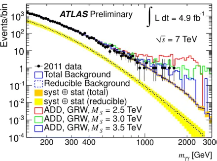
[GeV]
γ
mγ
200 300 400 1000 2000 3000
Events/bin
10
-410
-310
-210
-11 10 10
210
3ATLAS Preliminary
-1L dt = 4.9 fb
∫
= 7 TeV s
2011 data
Total Background Reducible Background
stat (total)
⊕ syst
stat (reducible)
⊕ syst
= 2.5 TeV M
SADD, GRW,
= 3.0 TeV M
SADD, GRW,
= 3.5 TeV M
SADD, GRW,
Figure 6: Observed invariant mass distribution of diphoton events, with the predicted SM background and expected signals for several ADD models superimposed.
[GeV]
γ
mγ
200 300 400 1000 2000 3000
Events/bin
10
-410
-310
-210
-11 10 10
210
3ATLAS Preliminary
-1L dt = 4.9 fb
∫
= 7 TeV s
2011 data
Total Background Reducible Background
stat (total)
⊕ syst
stat (reducible)
⊕ syst
= 1.25 TeV m
G= 0.1, M
PlRS, k/
= 1.5 TeV m
G= 0.1, M
PlRS, k/
= 1.75 TeV m
G= 0.1, M
PlRS, k/
Figure 7: Observed invariant mass distribution of diphoton events, with the predicted SM background
and expected signals for several RS models superimposed.
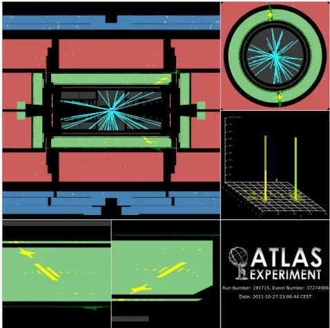
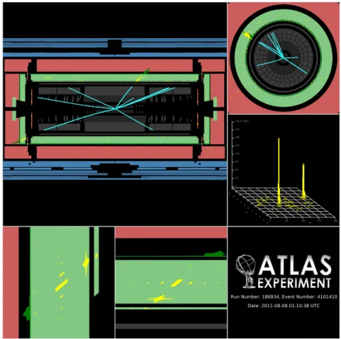
Figure 8: Event display of the highest-mass diphoton event. Event information: Run and event numbers
=
![Table 2: 95 % CL lower limits on the mass [TeV] of the lightest RS graviton, for various values of k/M Pl](https://thumb-eu.123doks.com/thumbv2/1library_info/4027321.1542198/10.892.225.673.110.219/table-lower-limits-mass-lightest-graviton-various-values.webp)