Combined measurements of the Higgs boson production and decay rates in H → Z Z ∗ → 4` and H → γγ final states using pp collision

A TLAS-CONF-2016-081 08 August 2016

ATLAS NOTE

ATLAS-CONF-2016-081

8th August 2016

Combined measurements of the Higgs boson production and decay rates in H → Z Z ^∗ → 4` and H → γγ final states using pp collision

data at √

s = 13 TeV in the ATLAS experiment

The ATLAS Collaboration

Abstract

This note presents combined measurements based on Higgs boson production cross sections and branching ratios using more than 13.3 fb ⁻¹ of proton-proton collision data recorded by the ATLAS experiment at the LHC at √

s = 13 TeV. The combination is based on the anal- yses of the H → γγ and H → ZZ ^∗ → 4` decay channels. Results are derived for these two decay modes and five sets of production processes for a Higgs boson rapidity |y H | < 2.5 and for a Higgs boson mass of 125.09 ± 0.21(stat) ± 0.11(syst) GeV. The global signal strength, defined as the ratio in the full phase space (including |y H | ≥ 2.5) between the observed total signal yield and the Standard Model expectation, is measured to be µ = 1.13 ⁺ _−0.17 ^0.18 . The cross section of pp → H + X in the full phase space is determined from fiducial cross section measurements to be 59.0 ⁺ _−9.2 ^9.7 (stat.) ^+4.4 _−3.5 (syst.) pb, to be compared with the Standard Model prediction of 55.5 ⁺ _−3.4 ^2.4 pb. No significant deviation from the Standard Model expectations is observed.

c

2016 CERN for the benefit of the ATLAS Collaboration.

Reproduction of this article or parts of it is allowed as specified in the CC-BY-4.0 license.

1 Introduction

This note presents combined measurements based on Higgs boson production cross sections and branch- ing ratios using proton-proton collision data produced by the LHC at a centre-of-mass energy of √

s = 13 TeV and recorded by the ATLAS detector. The analysis is based on the measurements performed in the indi- vidual H → γγ and H → ZZ ^∗ → 4` decay channels [1, 2].

Higgs boson production and decays were studied at √

s of 7 and 8 TeV and were found to be consistent with expectations from the Standard Model (SM) [3]. The data sample already collected so far at √

s = 13 TeV allows initial measurements with comparable precision. With the increased data sample that will be taken during the next years, these measurements will reach much higher precision and probe the Higgs sector in depth.

SM production of the Higgs boson at the LHC is dominated by the gluon fusion process gg → H, followed by the vector-boson fusion process qq ⁰ → qq ⁰ H. Associated production with a W boson q q ¯ ⁰ → W H, a Z boson q q/gg ¯ → ZH or with a pair of top quarks q q/gg ¯ → t¯ tH also have sizeable contributions. The W H and ZH production processes are collectively referred to as the V H process. Smaller contributions are expected from production in association with b quarks b bH ¯ and production in association with a single top quark (tH) with the latter proceeding through either the qb → tHq ⁰ or gb → WtH process. The theoretical calculations of the Higgs boson production cross sections and decay branching ratios have been compiled in Refs. [4–7]. The combined analysis considers five sets of production processes: ggF (gg → H and b bH), ¯ VBF (qq ⁰ → qq ⁰ H), VHhad (q q/gg ¯ → ZH and q q ¯ ⁰ → W H with hadronic decays of W /Z), VHlep (q q/gg ¯ → ZH and q q ¯ ⁰ → W H with decays of W /Z to charged leptons and / or neutrinos) and top (q q/gg ¯ → t¯ tH and tH).

Products of Higgs boson production cross sections of process i (σ i ) and branching ratios to the final state f (B ^f ), σ i · B ^f = (σ · B) i ^f (following the notation in Ref. [3]), are reported for |y H | < 2.5, where y H is the Higgs boson rapidity. This corresponds to the "stage-0" simplified template cross sections from Ref. [8]. For Higgs boson rapidity |y H | > 2.5, the H → γγ and H → ZZ ^∗ → 4` analyses have a negligible acceptance. The separation of the production processes is achieved by exploiting the di ff erences in event topologies and kinematics of the di ff erent production processes through categorisation of events. The results for (σ · B) <sub>ggF</sub> <sup>f</sup> and (σ · B) <sub>VBF</sub> <sup>f</sup> for H → γγ and H → ZZ <sup>∗</sup> → 4` are presented in the two-dimensional plane to show their correlation. In addition, production cross sections σ i for a Higgs boson rapidity

|y H | < 2.5 are measured by assuming the SM Higgs branching ratios to γγ and ZZ ^∗ , and by concurrently determining the ratio of the branching ratios to γγ and ZZ ^∗ .

A measurement of the global signal strength µ, which is defined as the ratio of the observed total signal yield to the total signal yield expected from the SM, used as a single scaling factor for all production processes and decay modes, is presented after extrapolation to the full phase space. The measurement is based on the same categorisation of events as the measurements introduced above to benefit from the sensitivity improvement of this technique.

Table 1 summarises the four di ff erent fit models based on event categorisation and the number of measured parameters in each fit model.

The measurement of the total cross section, extrapolated to the full phase space, based on the fiducial cross

section measurements in H → γγ and H → ZZ ^∗ → 4` follows a di ff erent strategy: instead of attempting

to separate the different Higgs boson production processes or using the categorisation to enhance the

sensitivity, the inclusive event samples are used to minimise the model dependence. Differences in the

Table 1: Summary of the fit strategies based on event categorisation used in this note.

Number of

Fit model parameters of interest Section

Independent σ i · B ^f 7 4.1

Independent σ i assuming SM B ^f 5 4.2

(σ · B) ^ZZ _ggF , σ VBF /σ ggF and B ^γγ /B ^ZZ 3 4.3

Global signal strength µ 1 5

acceptances and in the experimental effects between the different production modes are considered as systematic uncertainties in the measurement of the total cross section. All measurements are performed under the assumption that the Higgs boson mass is 125.09 ± 0.21(stat) ± 0.11(syst) GeV [9].

Section 2 introduces the data sample that the measurements presented are based on, gives an overview of the simulation samples for Higgs boson production, as well as a brief review of the analyses in the H → γγ and H → ZZ ^∗ → 4` decay channels. Section 3 provides a short introduction into the underlying statistical technique that is used. Sections 4-6 present the measurements as discussed above, and Section 7 gives a summary.

2 Analysis

2.1 Data sample

The proton-proton collision data were collected by the ATLAS experiment in 2015 and 2016, with the LHC operating at a centre-of-mass energy of 13 TeV. The ATLAS detector is described in detail else- where [10, 11].

The analysis only considers events taken during stable beam conditions and when the full detector was operational and delivered data of good quality. The dataset amounts to 13.3 fb ⁻¹ for the H → γγ analysis and to 14.8 fb ^{− 1} for the H → ZZ ^∗ → 4` analysis, of which 3.2 fb ^{− 1} were collected in 2015 and the rest in 2016. The mean number of proton-proton interactions per bunch crossing (also referred to as event pileup) was approximately equal to 14 in the 2015 dataset and to 22 in the 2016 dataset.

2.2 Samples of simulated Higgs boson events

Higgs boson production via gluon-gluon fusion (gg → H) is simulated at next-to-leading-order (NLO) accuracy in QCD using the P owheg B ox [12–15], with the CT10 parton distribution function (PDF) [16].

The mass and natural width of the Higgs boson are chosen to be m H = 125 GeV and Γ H = 4.07 MeV [6],

respectively. The parton-level events produced by the Powheg Box are passed to Pythia8 [17] to provide

parton showering, hadronisation and multiple parton interactions (MPI). The sample is normalised such

that it reproduces the total cross section predicted by a next-to-next-to-next-to-leading-order (N ³ LO)

QCD calculation with NLO electroweak corrections applied [7, 18–21]. Additional corrections are ap-

plied to the shape of the Higgs boson transverse momentum distribution to reproduce the distribution

predicted by H res 2.1 [22] at NNLO + NNLL, which includes the e ff ects of top- and bottom-quark masses and uses dynamical renormalisation and factorisation scales. To avoid a sizeable effect on the fraction of events with two or more jets and to preserve their consistency with the most precise available calculations, the corrections are computed after subtracting the transverse momentum spectrum of events with two or more jets from the simulation from the Hres2.1 prediction and the simulation. The reweighting is only applied to events with fewer than two jets.

Higgs boson production via vector-boson fusion (VBF: qq ⁰ → qq ⁰ H) is generated to NLO accuracy in QCD using the P owheg B ox [23] with the CT10 PDF. The parton-level events are passed to P ythia 8 to provide parton showering, hadronisation and MPI. The VBF sample is normalised to an approximate- NNLO QCD cross section with NLO electroweak corrections applied [7, 24–26]. Higgs boson production in association with a vector boson (V H: q q ¯ → ZH, q q ¯ ⁰ → W H) is produced at leading-order (LO) accuracy in QCD using P ythia 8 with the NNPDF2.3LO PDF set [27]. The samples are normalised to cross sections calculated at NNLO in QCD with NLO electroweak corrections [28, 29] including the NLO QCD corrections [30] for gg → ZH [7].

Higgs boson production in association with a top–antitop pair (q q/gg ¯ → t¯ tH) is produced at NLO accu- racy in QCD using MG5_aMC [31] with the NNPDF2.3 PDF and interfaced to Pythia8 to provide parton showering, hadronisation and MPI. The t¯ tH sample is normalised to a cross section calculation accurate to NLO in QCD with NLO electroweak corrections applied [7, 32–35].

Higgs boson production via bottom-quark fusion (b bH) is produced using MG5_aMC [36] interfaced ¯ to P ythia 8, and is normalised to a cross section calculation accurate to NNLO in QCD [7, 37–39]. The sample includes the e ff ect of interference with the gluon fusion production mechanism. Higgs boson production in association with a single top-quark and a W-boson (tHW ) is produced at LO accuracy using MG5_aMC interfaced to H erwig++ [40]. Higgs boson production in association with a single top- quark, a b-quark and a light quark (tH jb) is produced at LO accuracy using MG5_aMC interfaced to Pythia8. The tHW and tH jb samples are normalised to calculations accurate to NLO in QCD [7, 41].

The particle-level Higgs boson events are passed through a G eant 4 [42, 43] simulation of the ATLAS detector [44] and reconstructed using the same analysis software as used for the data. Event pileup is included in the simulation by adding inelastic proton–proton collisions, such that the average number of interactions per bunch crossing reproduces that observed in the data. The inelastic proton–proton collisions were produced using Pythia8.

2.3 Analyses in the individual decay channels

The event categorisation used for the results presented in Sections 4 and 5 is optimised for the best separation of the Higgs boson production processes. For each decay channel, the events are divided into a number of mutually exclusive categories based on reconstructed event kinematics and topology. These are defined such that each category is sensitive primarily to a given production mode. A further subdivision of the categories is made, based e.g. on the number of jets in the final state; details are given in Ref. [1, 2]

and a brief reminder is given in Sections 2.3.1 and 2.3.2 below. The Standard Model predictions for the

relative contribution of the di ff erent production modes to each category are taken as a "template". These

serve as the basis of the fit of the yields of di ff erent production modes times corresponding branching

ratios.

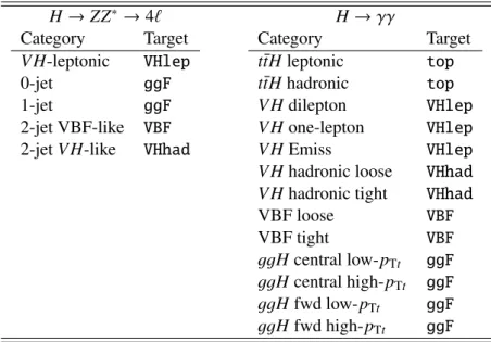
Table 2 gives an overview of the event categories for both decay modes used for the measurement of the simplified template cross sections and the inclusive signal strength, which is described in more detail in the following Sections.

Table 2: Categories entering in the combined measurements for the H → ZZ

→ 4` and H → γγ decay modes as described in [2] and [1] respectively. Each category is designed to separate a specific set of production processes, as summarised in the columns named target.

H → ZZ ^∗ → 4`

Category Target V H -leptonic VHlep

0-jet ggF

1-jet ggF

2-jet VBF-like VBF 2-jet V H -like VHhad

H → γγ

Category Target

t¯ tH leptonic top t¯ tH hadronic top

V H dilepton VHlep

V H one-lepton VHlep

V H Emiss VHlep

V H hadronic loose VHhad V H hadronic tight VHhad

VBF loose VBF

VBF tight VBF

ggH central low-p _Tt ggF ggH central high-p _Tt ggF ggH fwd low-p Tt ggF ggH fwd high-p _Tt ggF

2.3.1 H → Z Z ^∗ → 4`

The H → ZZ ^∗ → 4` analysis [1] reconstructs the Z and the Z ^∗ bosons in their decays to electrons and muons. It uses five event categories to separate the di ff erent Higgs boson production modes. The V H leptonic category requires the presence of at least one additional lepton. The remaining events are categorised according to their jet multiplicity into categories with zero, exactly one and at least two jets, and the two-jet category is split into a VBF- and a V H-enriched region using the dijet invariant mass.

In the jet-multiplicity based categories boosted decision trees (BDTs) based on the kinematic variables of jets and Z bosons are used to separate the different Higgs production processes from the SM ZZ ^∗ background. In the two-jet V H category, the BDT discriminant is designed to separate V H production from VBF and gluon fusion production, in the two-jet VBF category, the BDT is trained to separate VBF production from gluon fusion production, in the one-jet category the BDT discriminant is built to separate VBF production from gluon fusion production and SM ZZ ^∗ background, and in the zero-jet category the BDT is trained to separate the Higgs signal, dominated by gluon fusion production, from SM ZZ ^∗ background.

Only events with an invariant four-lepton mass between 118 and 129 GeV are considered in the analysis.

In the jet categories, the signal is extracted through a binned fit to the BDT discriminant, while the signal

estimation in the V H leptonic category is based on event counting. The remaining ZZ ^∗ → 4` background

is estimated from the Monte Carlo simulation, while the Z + jets and t¯ t backgrounds are estimated from

control regions in the data.

2.3.2 H → γγ

The H → γγ analysis [2] is based on 13 exclusive event categories targetting the five Higgs boson production modes introduced in Section 1. For categories enriched in t¯ tH production, the leptonic as well as fully hadronic decay signatures of the t¯ t system are considered. The leptonic selection requires at least one lepton, at least two jets and one of them should be identified as originating from a b-quark (b-tagged), as well as missing transverse momentum E ^miss _T or at least two b-tagged jets. In the hadronic selection, events with at least five jets with at least one b-tag are required. Five categories are enriched in V H production: the dilepton category requires two same-flavor, opposite-sign leptons consistent with a Z-boson decay; the one-lepton category requires exactly one lepton and a minimum E ^miss _T significance (defined as E _T ^miss / √ P

E _T , where P

E _T is the scalar sum of the transverse energies of all objects used in the estimation of the missing transverse momentum); the E _T ^miss category requires zero leptons, high E _T ^miss significance and a minimum diphoton transverse momentum; and the two hadronic V H categories require two jets consistent with a V decay and employ a BDT based on diphoton and dijet variables.

The selection of the two categories enriched in VBF events requires two jets loosely consistent with VBF topology and is based on a BDT combining six kinematic variables, among which the azimuthal di ff erence between the diphoton and the dijet system, ∆ φ _{γγ−j j} serves as an implicit third-jet veto. The remaining events are separated according to the pseudo-rapidity of the two photons and the p _Tt of the diphoton system (defined as the orthogonal component of the diphoton momentum when projected on the axis given by the difference of the momenta of the two photons, in analogy to Refs. [45, 46]), which separates events with different diphoton invariant mass resolution and further discriminates VBF and gluon fusion production.

The signal is extracted by a fit to the diphoton invariant mass distribution applied simultaneously to all event categories. The background shape is parameterised in each event category and determined from data.

3 Statistical model

The statistical treatment is described in Refs. [3, 47–51]. The parameters of interest each represent a product of a Higgs production cross section and a branching ratio in the fit described in Section 4.1, and reparameterisations thereof in the fits described in Sections 4.2, 4.3, and 5. In the present analysis we consider the five sets of production modes introduced in Section 1 (ggF, VBF, VHhad, VHlep, and top), and detailed further in Section 4, and two Higgs decay channels (ZZ ^∗ and γγ), giving initially 10 parameters to be estimated. For the fit described in Section 6, the parameter of interest is the inclusive Higgs production cross section (no split by production processes) times branching ratio.

These parameters can be used to predict the mean numbers of events in bins corresponding to different kinematic regions for several event topologies. These regions are designed to be sensitive primarily to a given Higgs boson production mode and decay channel, as described in Section 2.3. An exception is the fit described in Section 6, which does not rely on event categorisation, and uses only one bin. A likelihood function is constructed that treats the number of events found in each bin as an independent Poisson-distributed value, or is based on the unbinned diphoton invariant mass distribution in the case of low-statistics event categories in H → γγ.

The predicted mean number of events in each bin depends as well on additional nuisance parameters,

related to the uncertainty on the electromagnetic and jet energy scale systematic uncertainties, luminosity,

background shape, etc. In total there are about 200 nuisance parameters, which are determined by the fit, although their values themselves are not of particular interest. Some of these are constrained by the same data. Other nuisance parameters are constrained by auxiliary information such as independent control measurements. In this case, the estimated value of the nuisance parameter is constrained by either a Gaussian or a log-normal distribution, and a corresponding multiplicative term is included in the likelihood function (further details can be found in Refs. [47, 48]). Uncertainties are treated as either uncorrelated or fully (anti-)correlated. Uncertainties that are fully (anti-)correlated between di ff erent event categories or between different decay channels share the same nuisance parameter.

The sources of theoretical uncertainties related to the Higgs boson signal considered in the measurements of the cross sections are uncertainties in the acceptance of the different categories due to missing higher- order QCD corrections, uncertainties in the PDFs [52, 53], and uncertainties in the modelling of the underlying event and parton shower (UE / PS). The nuisance parameter related to the uncertainties due to missing higher-order QCD correction for the inclusive 2-jet acceptance in the VBF categories is shared between H → γγ and H → ZZ ^∗ → 4`, and so is the nuisance parameter associated to the effect of the uncertainties due to missing higher-order QCD correction in the splitting of the signal in the p <sub>Tt</sub> categories [22, 54] in H → γγ and the 0- and 1-jet categories [55–57] in H → ZZ <sup>∗</sup> → 4`. The nuisance parameters associated with UE/PS uncertainties are also correlated between the two decay channels.

For the measurement of the signal strength, uncertainties on the predicted cross section are taken into account, including uncertainties from missing higher-order QCD corrections, as well as uncertainties on the PDFs and α s . These uncertainties are fully correlated between the different decay channels. In addition, theoretical and parametric uncertainties on the decay branching ratios are included [7, 58–61].

The correlation scheme for these systematic uncertainties follows the strategy reported in Ref. [3]. All the experimental sources of uncertainties shared by the two analyses are correlated in the combined fit, notably the uncertainties on the electromagnetic energy scale and resolution, the muon energy scale, the jet energy scale and resolution, as well as uncertainties related to the reconstruction and isolation efficiencies of electrons, and the uncertainties related to the identification and isolation efficiencies of muons.

The statistical procedure results in a likelihood function L(α, θ), where α represents the 10 parameters of interest and θ is the set of nuisance parameters. A statistical test of hypothetical α values is carried out using the profile likelihood ratio [62]

Λ (α) = L(α, θ(α)) ˆˆ

L( ˆ α, θ) ˆ . (1)

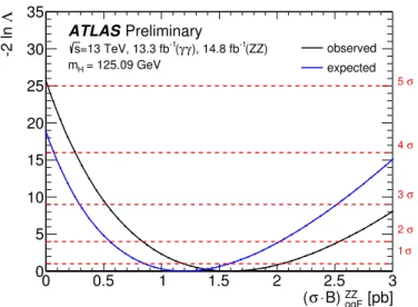
In the numerator, the nuisance parameters are varied to maximise the likelihood function for given fixed values of the parameters of interest α (conditional maximum-likelihood). In the denominator, both the parameters of interest and the nuisance parameters are varied to maximise the likelihood function (un- conditional maximum-likelihood). The choice of the parameters of interest depends on the test under consideration, with the remaining parameters being “profiled", i.e., similarly to nuisance parameters they are set to the values that maximise the likelihood function for the given fixed values of the parameters of interest. Asymptotically, a test statistic −2 ln Λ (α) of several parameters of interest α is distributed as a χ ² distribution with n degrees of freedom, where n is the dimensionality of the vector α. An example for the distribution of −2 ln Λ(α) for the measurement of (σ · B) ^ZZ _ggF described in Section 4 is shown in Figure 1.

All results presented in the following Sections are based on likelihood evaluations and give confidence

level (CL) intervals assuming the asymptotic approximation.

[pb]

ZZ

( σ ⋅ B)

0 0.5 1 1.5 2 2.5 3

Λ -2 ln

0 5 10 15 20 25 30 35

1 σ 2 σ σ 3 4 σ 5 σ

Preliminary ATLAS

-1(ZZ) ), 14.8 fb γ (γ

=13 TeV, 13.3 fb-1

s

= 125.09 GeV mH

observed expected

Figure 1: −2 ln Λ (α) scan for the measurement of (σ · B)

described in Section 4. The number of degrees of freedom in this example is ndf = 1, and the intervals defined by the intersections with the dashed lines are the confidence level intervals for about 68.3% (1 σ), 95.4% (2 σ), 99.7% (3 σ) and higher than 99.99% (4 and 5 σ) respectively.

The compatibility with the Standard Model, p _SM , is quantified using the p-value [62] ¹ obtained from the value of −2 ln Λ (α = α _SM ), where α is the set of parameters of interest and α _SM are their Standard Model values, and assuming asymptotic χ ² distribution with a number of degrees of freedom equal to the number of parameters of interest of the test statistic.

4 Combined results for cross sections and branching ratios

The combined analysis of the di ff erent decay channels is performed in the statistical framework intro- duced in Section 3, with (σ · B) i ^f = σ i · B ^f as parameters of interest, where σ i is the cross section for production process i (for |y H | < 2.5, referred to as “central” below), B ^f is the branching fraction for the final state f .

The sets of production modes considered were introduced in Section 1: ggF, VBF, VHhad, VHlep and top.

With the present data sample and the decay channels taken into account, the combined analysis is only sensitive to a subset of all possible production processes, which motivates the grouping of production processes as follows:

• b bH ¯ is coupled with gg → H by assuming SM predictions for the ratio of the two processes, and the combined cross section of the two processes will be reported, labelled “ggF”.

• tH is coupled with t¯ tH, by assuming SM predictions for the ratio of the pp → tH and the pp → t¯ tH cross sections, together reported as “top”.

1

The p-value is defined as the probability to obtain a value of the test statistic that is at least as high as the observed value,

under the hypothesis that is being tested.

• W H and ZH are merged, separately for the hadronic V and the leptonic (including charged leptons and neutrinos) decays, into V(→ q q)H ¯ and V (→ leptons)H, reported as “VHhad” and “VHlep” , respectively. The merging assumes the SM prediction for the ratio of the production cross sections and includes the contributions from both q q ¯ → V H and gg → ZH.

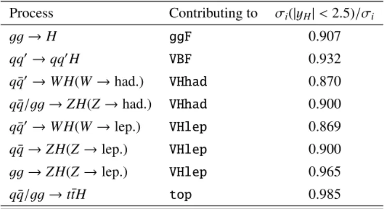
Table 3 shows the value of the fraction between the central and the total cross section per production pro- cess, calculated using the simulated samples described in Section 2.2. These fractions, and the theoretical calculations in Ref. [7], are used to calculate the values of the SM prediction for the measured cross sections shown in the following Sections.

In the models considered below, the original parameters of interest, (σ·B) i ^f , are determined in the analysis described in Section 4.1. For the analyses described in Sections 4.2 and 4.3 the respective parameters of interest are expressed in terms of the (σ · B) i ^f . Theoretical uncertainties are included for those quantities that are fixed to the SM predictions.

Table 3: Ratio between the central and the total cross section per production process. The uncertainties related to the finite size of the simulated samples used to calculate the fractions are of the order of 5% , and not reported in the table. The values of the fraction between the central and the total cross section for b bH ¯ and tH are assumed to have a negligible impact on the calculation of the SM predictions shown in the following Sections, and they are set to one.

Process Contributing to σ

(|y

| < 2.5)/σ

gg → H ggF 0.907

qq

→ qq

H VBF 0.932

q q ¯

→ W H(W → had.) VHhad 0.870

q q/gg ¯ → ZH(Z → had.) VHhad 0.900

q q ¯

→ W H(W → lep.) VHlep 0.869

q q ¯ → ZH(Z → lep.) VHlep 0.900

gg → ZH(Z → lep.) VHlep 0.965

q q/gg ¯ → t tH ¯ top 0.985

4.1 Parameterisation using independent products of cross sections and branching fractions

The first model provides measurements for a total of seven of the (σ·B) i ^f : the product of the cross sections

for ggF (σ ggF ), VBF (σ VBF ), VHhad (σ VHhad ), VHlep (σ VHlep ) and top (σ top ) are measured in the central

region, with the branching fractions into γγ and ZZ ^∗ . While the measured (σ · B) i ^f are for the specific

final state f , the combined analysis allows for a correlation of the systematic uncertainties as described

in Section 3. Among the ten (σ · B) i ^f , the three that are not well enough constrained from data are fixed to

the respective SM predictions: (σ · B) ^ZZ _VHhad , (σ · B) ^ZZ _VHlep and (σ · B) ^ZZ _top . The H → ZZ ^∗ → 4` analysis does

not have any event category sensitive to Higgs boson production in association with top quarks, and very

few events in the categories sensitive to V H production. Measurements are obtained for the parameters of

interest given in Table 4. Theoretical uncertainties on the predicted SM cross section ratios that are fixed

in the analysis as described above are taken into account. The combination of the nuisance parameters

due to the assumptions on the correlation scheme between the H → ZZ ^∗ → 4` and the H → γγ analyses, and the specific definition of ggF, VBF VHhad, VHhad and top generate the small differences between the results in Table 5 and the ones presented in Ref. [1] and Ref. [2].

Table 4: Parameters of interest for the measurement of (σ · B)

.

Decay mode ggF VBF VHhad VHlep top

H → γγ (σ · B)

(σ · B)

(σ · B)

(σ · B)

(σ · B)

H → ZZ

(σ · B)

(σ · B)

fixed to SM fixed to SM fixed to SM

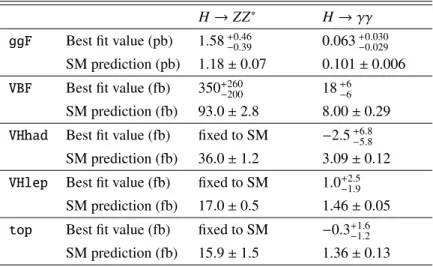
Table 5: Best fit values of (σ · B)

for each specific channel i → H → f , as obtained from the generic parameteri- sation with 7 parameters as given in Table 4. The SM predictions [7] are shown for each (σ · B)

.

H → ZZ

H → γγ ggF Best fit value (pb) 1.58

0.063

SM prediction (pb) 1.18 ± 0.07 0.101 ± 0.006 VBF Best fit value (fb) 350

18

SM prediction (fb) 93.0 ± 2.8 8.00 ± 0.29 VHhad Best fit value (fb) fixed to SM −2.5

SM prediction (fb) 36.0 ± 1.2 3.09 ± 0.12 VHlep Best fit value (fb) fixed to SM 1.0

SM prediction (fb) 17.0 ± 0.5 1.46 ± 0.05 top Best fit value (fb) fixed to SM −0.3

SM prediction (fb) 15.9 ± 1.5 1.36 ± 0.13

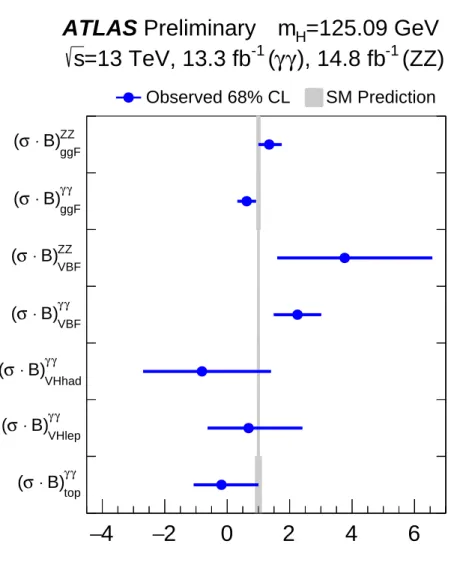
Figure 2 shows the cross sections (σ · B) i ^f as given in Table 4 for ggF, VBF, VHhad, VHlep and top measured in H → γγ and H → ZZ ^∗ . The fit results displayed are normalised to the SM predictions for the various parameters and the grey bands indicate the theoretical uncertainties in these predictions. A summary of the measured cross sections (σ · B) i ^f is shown in Table 5.

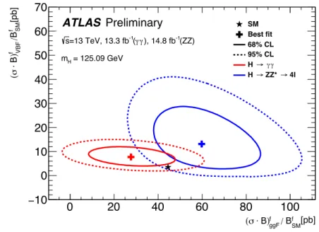
The ggF and VBF cross sections are measured with the best precision. As the event categories from which they are mainly constrained typically have substantial contributions from both gg → H and VBF, the measured cross sections of the two sets of production modes are correlated. To compare the contours in the (σ · B) _ggF ^f –(σ · B) _VBF ^f plane, as measured in H → γγ and H → ZZ ^∗ when the remaining parameters of interest are profiled, the values of (σ · B) i ^f are divided by the branching fraction for the decay mode f predicted by the SM, B _SM ^f , as shown in Figure 3.

The uncertainties on the electromagnetic energy resolution and the photon identification e ffi ciency play

the most important role among the experimental errors. The uncertainties on the acceptance of gluon

fusion production in the categories with a specific number of jets in the event are the most prominent

theoretical uncertainties.

Parameter value norm. to SM value

− 4 − 2 0 2 4 6

γ γ

B) top

⋅ σ (

γ γ VHlep

⋅ B) σ (

γ γ VHhad

⋅ B) σ (

γ γ

B) VBF

⋅ σ (

ZZ

B) VBF

⋅ σ (

γ γ

B) ggF

⋅ σ (

ZZ

B) ggF

⋅ σ (

ATLAS Preliminary m _H =125.09 GeV (ZZ) ), 14.8 fb -1

γ γ

-1 (

=13 TeV, 13.3 fb s

Observed 68% CL SM Prediction

Figure 2: Cross sections (σ · B)

as given in Table 4 for ggF, VBF, VHhad, VHlep and top measured in H → γγ and H → ZZ

. The fit results are normalised to the SM predictions for the various parameters and the grey bands indicate the theoretical uncertainties in these predictions. The blue error bars show the full uncertainty, including experimental uncertainties and theoretical uncertainties that impact the measurements.

The compatibility between the measurement and the SM prediction corresponds to a p-value of p _SM = 11%.

4.2 Parameterisation using independent production cross sections and assuming SM Higgs decay branching fractions

The second model focuses on the measurement of the production cross sections assuming SM Higgs decay

branching fractions. In this model, the cross sections for ggF (σ ggF ), VBF (σ VBF ), VHhad (σ VHhad ), VHlep

(σ VHlep ) and top (σ top ) are measured in the central region. Theoretical uncertainties on the predicted SM

SM

[pb]

f f

(σ ⋅ B ) /

B

0 20 40 60 80 100

[pb]

( σ ⋅ B ) / B

− 10 0 10 20 30 40 50 60 70

SM Best fit 68% CL 95% CL γ γ

→ H

→4l

→ZZ*

H

ATLAS Preliminary

-1

(ZZ) ), 14.8 fb γ γ

-1

(

=13 TeV, 13.3 fb s

= 125.09 GeV m

Figure 3: Contours in the (σ · B)

/B

–(σ · B)

/B

plane as measured in H → γγ and H → ZZ

, together with the SM prediction.

branching fractions and assumed SM cross section ratios as described above are taken into account.

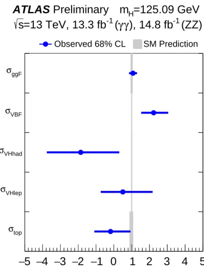
Figure 4 and Table 6 show the cross sections for ggF, VBF, VHhad, VHlep and top. The fit results displayed in Figure 4 are normalised to the SM predictions for the various parameters and the grey bands indicate the theoretical uncertainties in these predictions.

The compatibility between the measurement and the SM prediction corresponds to a p-value of p _SM = 21%.

Table 6: Best fit values of the production cross sections σ

assuming SM Higgs decay branching fractions. The SM predictions [7] are shown for each σ

.

Best fit value (pb) SM prediction (pb)

σ

47.8

44.5 ± 2.3

σ

7.9

3.52 ± 0.07

σ

− 2.5

1.36 ± 0.03

σ

0.32

0.64 ± 0.02

σ

−0.11

0.60 ± 0.06

Parameter value norm. to SM value

− 5 − 4 − 3 − 2 − 1 0 1 2 3 4 5

σ top VHlep

σ

VHhad

σ σ VBF

σ ggF

ATLAS Preliminary m _H =125.09 GeV (ZZ) ), 14.8 fb -1

γ γ

-1 (

=13 TeV, 13.3 fb s

Observed 68% CL SM Prediction

Figure 4: Cross sections for ggF, VBF, VHhad, VHlep and top measured with the assumption of SM branching fractions. The fit results are normalised to the SM predictions for the various parameters and the grey bands indicate the theoretical uncertainties in these predictions. The blue error bars show the full uncertainty, including experimental uncertainties and theoretical uncertainties that impact the measurements.

4.3 Parameterisation using ratios of cross sections and of branching fractions

The third model provides measurements of ratios of cross sections and of branching fractions extracted from a combined fit to the data by normalising the production cross section for process i to ggF and the branching ratio for final state f to B ^ZZ . The product of the cross section and the branching fraction (σ · B) _i ^f can then be expressed using the ratios as:

(σ · B) _i ^f = (σ · B) ^ZZ _ggF · σ i

σ ggF

!

· B ^f B ^ZZ

!

, (2)

where the σ i are the cross sections considered in Section 4.2. With the present data sample and the decay channels taken into account, the combined analysis is only sensitive to (σ·B) ^ZZ _ggF , σ VBF /σ ggF and B ^γγ /B ^ZZ . In the combined fit, the remaining ratios between cross sections and ggF are profiled.

Parameter value norm. to SM value

0 1 2 3 4 5

σ ggF VBF / σ

/B ZZ γ

B γ ZZ

B) ggF

⋅ σ (

ATLAS Preliminary m _H =125.09 GeV (ZZ) ), 14.8 fb -1

γ γ

-1 (

=13 TeV, 13.3 fb s

Observed 68% CL SM Prediction

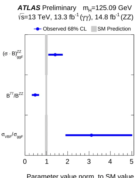
Figure 5: Measurement of (σ·B)

, σ

/σ

and B

/B

. The fit results are normalised to the SM predictions for the various parameters and the grey bands indicate the theoretical uncertainties in these predictions. The remaining ratios between production cross sections and ggF are profiled in the combined fit. The blue error bars show the full uncertainty, including experimental uncertainties and theoretical uncertainties that impact the measurements.

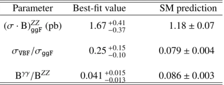
Figure 5 shows the measurement of (σ · B) ^ZZ _ggF , σ VBF /σ ggF and B ^γγ /B ^ZZ compared to their SM expectation.

The fit results displayed in Figure 5 are normalised to the SM predictions for the various parameters and the grey bands indicate the theoretical uncertainties in these predictions.

The compatibility between the measurement and the SM prediction corresponds to a p-value of p _SM = 5%.

Evidence for the the vector-boson fusion production process is established at √

s = 13 TeV, with a local

significance of 4.0 σ (1.9 σ expected), based on the value of −2 ln Λ (σ VBF /σ ggF = 0) and assuming asymptotic distribution of the test statistic.

Table 7: Best-fit values of the cross section (σ· B)

and of the ratios σ

/σ

and B

/B

. The remaining ratios between production cross sections and ggF are profiled in the combined fit. The SM predictions [7] are shown in the last column.

Parameter Best-fit value SM prediction (σ · B) ^ZZ _ggF (pb) 1.67 ⁺ _−0.37 ^0.41 1.18 ± 0.07

σ VBF /σ ggF 0.25 ⁺ _−0.10 ^0.15 0.079 ± 0.004 B ^γγ /B ^ZZ 0.041 ⁺ _−0.013 ^0.015 0.086 ± 0.003

5 Signal strength measurements

The global signal strength µ is determined, following the measurements performed at √

s = 7 and 8 TeV [3]. It is a single parameter, defined as the ratio of the observed yield and its SM expectation

µ = σ × B

(σ × B) ^SM , (3)

and is a single scaling factor for all production processes and decay modes, after extrapolation to the full phase space (including |y H | ≥ 2.5). It depends on the SM predictions for each production mode cross section and decay branching ratio, and the uncertainties on these predictions are folded into the measurement as described in Section 3.

Higgs boson production is observed in the analysed dataset with a local significance of about 10 σ (8.6 σ expected) , based on the value of −2 ln Λ (µ = 0) and assuming asymptotic distribution of the test statistic.

The global signal strength is measured to be µ = 1.13 ⁺ _−0.17 ^0.18 . The compatibility between the measurement and the SM prediction corresponds to a p-value of p _SM = 43%.

6 Combination of total cross sections

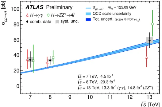
The measurements of the total cross section are based on the measured inclusive signal yields, and no attempt is made to disentangle the different Higgs boson production modes. The event yields measured in H → γγ [2] and H → ZZ ^∗ → 4` [1] decays are corrected for detector e ff ects, fiducial acceptances, and branching ratios. The corrections are derived assuming that the cross-section ratios between the different production modes follow the SM prediction. Uncertainties are assigned on this assumption by allowing for variations consistent with Ref. [3]. The combination of the two decay channels is performed using the statistical framework presented in Section 3.

Results are presented for centre-of-mass energies of 7, 8, and 13 TeV, corresponding to integrated lumi-

nosities of 4.5 fb ^{− 1} , 20.3 fb ^{− 1} and 13.3 fb ⁻¹ (H → γγ) – 14.8 fb ⁻¹ (H → ZZ ^∗ → 4`), respectively. The

measurements at 7 and 8 TeV are taken from Ref. [63]. The measured cross sections probe the properties of the Higgs boson and can be compared to state-of-the-art theoretical calculations at the three different centre-of-mass energies.

[TeV]

s

7 8 9 10 11 12 13

[pb] H → pp σ

0 20 40 60 80

100 ATLAS Preliminary σ

m

= 125.09 GeV QCD scale uncertainty

s) PDF+α (scale ⊕

Tot. uncert.

γ γ

H → H → ZZ * → 4 l comb. data syst. unc.

= 7 TeV, 4.5 fb

s

= 8 TeV, 20.3 fb

s

*) ZZ

-1

( ), 14.8 fb γ

γ

-1

( = 13 TeV, 13.3 fb s

Figure 6: Total pp → H + X cross sections measured at di ff erent centre-of-mass energies compared to Standard Model predictions at up to N

LO in QCD. The red triangles show the measurements from the H → γγ channel, the green rectangles show the measurements from the H → ZZ

→ 4` channel, and the black dots show the combina- tions of these two channels. The grey bands on the combined measurements represent the systematic uncertainty, while the black lines are the total uncertainty. The SM predictions (for a Higgs boson mass of 125.09 GeV [9]) are shown as a smooth curve, which is obtained by applying a third-order polynomial fit to the values available in Ref. [7]. The light (dark) blue band shows the uncertainty from missing higher-order QCD corrections (total uncertainty). The theoretical uncertainties are partially correlated between di ff erent values of the centre-of-mass energy.

The total pp → H + X cross sections at centre-of-mass energies of 7, 8 and 13 TeV measured in H → γγ and H → ZZ ^∗ → 4` are shown in Table 8 and Figure 6, along with their combination. For comparison, the SM predictions for the total cross section at the three centre-of-mass energies are given. To derive the breakdown of the uncertainties, the statistical uncertainties are obtained by fixing all nuisance parameters for the systematic uncertainties to their best-fit values and taking the quadratic di ff erence with respect to the result of the fit where all parameters are allowed to vary. The systematic uncertainties are smaller than the statistical uncertainties for the measurements at all three center-of-mass energies. The results of the two decay channels are compatible within the quoted uncertainties, and no deviation from the SM predictions is observed.

7 Conclusions

Combined measurements based on Higgs boson production cross sections and branching ratios using proton-proton collision data produced by the LHC at √

s = 13 TeV and recorded by the ATLAS detector

Table 8: Total pp → H + X cross sections measured using H → γγ and H → ZZ

→ 4` decays, and their combination, for centre-of-mass energies of 7, 8 and 13 TeV. The SM predictions [7] are computed for a Higgs boson mass of 125.09 GeV [9].

Decay channel Total cross section (pp → H + X)

√ s =7 TeV √

s =8 TeV √

s =13 TeV

H → γγ 35

pb 30.5

pb 37

pb H → ZZ

→ 4` 33

pb 37

pb 81

pb Combination 34 ± 10 (stat.)

(syst.) pb 33.3

(stat.)

(syst.) pb 59.0

(stat.)

(syst.) pb

SM predictions [7] 19.2 ± 0.9 pb 24.5 ± 1.1 pb 55.5

pb

are presented. The analysis is based on the measurements performed in the individual H → γγ and H → ZZ ^∗ decay channels.

Higgs boson production is observed in the 13 TeV dataset with a local significance of about 10 σ (8.6 σ expected), and evidence for production via vector boson fusion is seen with a local significance of about 4 σ (1.9 σ expected).

Products of Higgs boson production cross sections and branching ratios are measured for a Higgs boson rapidity |y H | <2.5 for five sets of production processes, ggF, VBF, VHhad, VHlep, and top. In addition, production cross sections are measured by assuming the SM Higgs branching ratios to γγ and ZZ ^∗ , and by concurrently determining the ratio of the branching ratios to γγ and ZZ ^∗ .

The global signal strength, defined as as the ratio of the observed total signal yield to the SM expectation, is measured to be µ = 1.13 ⁺ _−0.17 ^0.18 .

The cross section of pp → H + X in the full phase space is determined from fiducial cross section measurements to be 59.0 ⁺ _−9.2 ^9.7 (stat.) ⁺ _−3.5 ^4.4 (syst.) pb. Using also previous measurements at 7 and 8 TeV, the centre-of-mass dependence of the total Higgs production cross section is compared to theoretical predictions.

No significant deviation from the Standard Model predictions is observed.

References

[1] The ATLAS Collaboration, Study of the Higgs boson properties and search for high-mass scalar resonances in the H → ZZ ^∗ → 4` decay channel at √

s = 13 TeV with the ATLAS detector, ATLAS-CONF-2016-079 (2016).

[2] The ATLAS Collaboration, Measurement of fiducial, di ff erential and production cross sections in the H → γγ decay channel with 9.5 fb ⁻¹ of 13 TeV proton-proton collision data,

ATLAS-CONF-2016-067 (2016).

[3] The ATLAS and CMS Collaborations,

Measurements of the Higgs boson production and decay rates and constraints on its couplings from a combined ATLAS and CMS analysis of the LHC pp collision data at √

s = 7 and 8 TeV,

(2016), arXiv:1606.02266 [hep-ex].

[4] LHC Higgs Cross Section Working Group et al.,

Handbook of LHC Higgs Cross Sections: 1. Inclusive Observables, CERN-2011-002 (CERN, Geneva, 2011), arXiv:1101.0593 [hep-ph].

[5] LHC Higgs Cross Section Working Group et al.,

Handbook of LHC Higgs Cross Sections: 2. Di ff erential Distributions, CERN-2012-002 (CERN, Geneva, 2012), arXiv:1201.3084 [hep-ph].

[6] LHC Higgs Cross Section Working Group et al.,

Handbook of LHC Higgs Cross Sections: 3. Higgs Properties,

CERN-2013-004 (CERN, Geneva, 2013), arXiv:1307.1347 [hep-ph].

[7] LHC Higgs Cross Section Working Group et al., ‘In preparation’,

https://twiki.cern.ch/twiki/bin/view/LHCPhysics/CERNYellowReportPageAt13TeV.

[8] J. R. Andersen et al.,

Les Houches 2015: Physics at TeV Colliders Standard Model Working Group Report, (2016), arXiv:1605.04692 [hep-ph].

[9] The ATLAS and CMS Collaborations, Combined Measurement of the Higgs Boson Mass in pp Collisions at √

s = 7 and 8 TeV with the ATLAS and CMS Experiments, Phys. Rev. Lett. 114 (2015) 191803, arXiv:1503.07589 [hep-ex].

[10] The ATLAS Collaboration, The ATLAS Experiment at the CERN Large Hadron Collider, JINST 3 (2008) S08003.

[11] M. Capeans et al., ATLAS Insertable B-layer Technical Design Report, CERN-LHCC-2010-013, ATLAS-TDR-19 (2010).

[12] P. Nason, A New method for combining NLO QCD with shower Monte Carlo algorithms, JHEP 0411 (2004) 040, arXiv:hep-ph/0409146 [hep-ph].

[13] S. Frixione, P. Nason and C. Oleari,

Matching NLO QCD computations with Parton Shower simulations: the POWHEG method, JHEP 0711 (2007) 070, arXiv:0709.2092 [hep-ph].

[14] S. Alioli et al., A general framework for implementing NLO calculations in shower Monte Carlo programs: the POWHEG BOX, JHEP 1006 (2010) 043, arXiv:1002.2581 [hep-ph].

[15] S. Alioli et al., NLO Higgs boson production via gluon fusion matched with shower in POWHEG, JHEP 0904 (2009) 002, arXiv:0812.0578 [hep-ph].

[16] H.-L. Lai et al., New parton distributions for collider physics, Phys. Rev. D82 (2010) 074024, arXiv:1007.2241 [hep-ph].

[17] T. Sjöstrand, S. Mrenna and P. Z. Skands, A Brief Introduction to PYTHIA 8.1, Comput. Phys. Commun. 178 (2008) 852, arXiv:0710.3820 [hep-ph].

[18] C. Anastasiou et al., Higgs Boson Gluon-Fusion Production in QCD at Three Loops, Phys. Rev. Lett. 114 (2015) 212001, arXiv:1503.06056 [hep-ph].

[19] C. Anastasiou et al.,

High precision determination of the gluon fusion Higgs boson cross-section at the LHC, JHEP 05 (2016) 058, arXiv:1602.00695 [hep-ph].

[20] S. Actis et al., NLO electroweak corrections to Higgs boson production at hadron colliders,

Phys. Lett. B670 (2008) 12, arXiv:0809.1301 [hep-ph].

[21] C. Anastasiou, R. Boughezal and F. Petriello,

Mixed QCD-electroweak corrections to Higgs boson production in gluon fusion, JHEP 04 (2009) 003, arXiv:0811.3458 [hep-ph].

[22] M. Grazzini and H. Sargsyan, Heavy-quark mass e ff ects in Higgs boson production at the LHC, JHEP 1309 (2013) 129, arXiv: 1306.4581 [hep-ph] .

[23] P. Nason and C. Oleari,

NLO Higgs boson production via vector-boson fusion matched with shower in POWHEG, JHEP 02 (2010) 037, arXiv:0911.5299 [hep-ph].

[24] M. Ciccolini, A. Denner and S. Dittmaier, Strong and electroweak corrections to the production of Higgs + 2-jets via weak interactions at the LHC, Phys. Rev. Lett. 99 (2007) 161803,

arXiv:0707.0381 [hep-ph].

[25] M. Ciccolini, A. Denner and S. Dittmaier,

Electroweak and QCD corrections to Higgs production via vector-boson fusion at the LHC, Phys. Rev. D77 (2008) 013002, arXiv:0710.4749 [hep-ph].

[26] P. Bolzoni et al., Higgs production via vector-boson fusion at NNLO in QCD, Phys. Rev. Lett. 105 (2010) 011801, arXiv:1003.4451 [hep-ph].

[27] R. D. Ball et al., Parton distributions with LHC data, Nucl. Phys. B867 (2013) 244, arXiv:1207.1303 [hep-ph].

[28] O. Brein, A. Djouadi and R. Harlander,

NNLO QCD corrections to the Higgs-strahlung processes at hadron colliders, Phys. Lett. B579 (2004) 149, arXiv:hep-ph/0307206 [hep-ph].

[29] A. Denner et al., Electroweak corrections to Higgs-strahlung o ff W / Z bosons at the Tevatron and the LHC with HAWK, JHEP 1203 (2012) 075, arXiv:1112.5142 [hep-ph].

[30] L. Altenkamp et al., Gluon-induced Higgs-strahlung at next-to-leading order QCD, JHEP 1302 (2013) 078, arXiv:1211.5015 [hep-ph].

[31] J. Alwall et al., The automated computation of tree-level and next-to-leading order di ff erential cross sections, and their matching to parton shower simulations,

JHEP 07 (2014) 079, Predictions quoted in this paper derived by the authors., arXiv:1405.0301 [hep-ph].

[32] W. Beenakker et al., NLO QCD corrections to t tH production in hadron collisions, ¯ Nucl. Phys. B653 (2003) 151, arXiv:hep-ph/0211352 [hep-ph].

[33] S. Dawson et al.,

Associated Higgs production with top quarks at the large hadron collider: NLO QCD corrections, Phys. Rev. D68 (2003) 034022, arXiv:hep-ph/0305087 [hep-ph].

[34] Y. Zhang et al.,

QCD NLO and EW NLO corrections to t tH production with top quark decays at hadron collider, ¯ Phys. Lett. B738 (2014) 1, arXiv:1407.1110 [hep-ph].

[35] S. Frixione et al.,

Weak corrections to Higgs hadroproduction in association with a top-quark pair, JHEP 1409 (2014) 065, arXiv:1407.0823 [hep-ph].

[36] M. Wiesemann et al., Higgs production in association with bottom quarks, JHEP 02 (2015) 132,

arXiv:1409.5301 [hep-ph].

[37] S. Dawson et al., Exclusive Higgs boson production with bottom quarks at hadron colliders, Phys. Rev. D69 (2004) 074027, arXiv:hep-ph/0311067 [hep-ph].

[38] S. Dittmaier, M. Krämer and M. Spira,

Higgs radiation o ff bottom quarks at the Tevatron and the CERN LHC, Phys. Rev. D70 (2004) 074010, arXiv: hep-ph/0309204 [hep-ph] . [39] R. V. Harlander and W. B. Kilgore,

Higgs boson production in bottom quark fusion at next-to-next-to leading order, Phys. Rev. D68 (2003) 013001, arXiv:hep-ph/0304035 [hep-ph].

[40] S. Gieseke et al., Herwig ++ 1.0: An Event generator for e + e- annihilation, JHEP 02 (2004) 005, arXiv:hep-ph/0311208 [hep-ph].

[41] F. Demartin et al., Higgs production in association with a single top quark at the LHC, Eur. Phys. J. C75 (2015) 267, arXiv:1504.00611 [hep-ph].

[42] S. Agostinelli et al., GEANT4: a simulation toolkit, Nucl. Instrum. Methods 506 (2003) 250.

[43] J. Allison et al., GEANT4 Developments and Applications, IEEE Trans. Nucl. Sci. 53 (2006) 270.

[44] The ATLAS Collaboration, The ATLAS Simulation Infrastructure, Eur. Phys. J. C70 (2010) 823, arXiv:1005.4568 [physics.ins-det].

[45] K. Ackersta ff et al., Search for anomalous production of dilepton events with missing transverse momentum in e ⁺ e ⁻ collisions at √

s = 161-GeV and 172-GeV, Eur.Phys.J. C4 (1998) 47, arXiv:hep-ex/9710010 [hep-ex].

[46] M. Vesterinen and T. Wyatt, A Novel Technique for Studying the Z Boson Transverse Momentum Distribution at Hadron Colliders, Nucl.Instrum.Meth. A602 (2009) 432,

arXiv:0807.4956 [hep-ex].

[47] The ATLAS Collaboration, Combined search for the Standard Model Higgs boson in pp collisions at √

s = 7 TeV with the ATLAS detector, Phys. Rev. D86 (2012) 032003, arXiv: 1207.0319 [hep-ex] .

[48] The ATLAS and CMS Collaborations,

Procedure for the LHC Higgs boson search combination in Summer 2011, ATL-PHYS-PUB-2011-011, CERN-CMS-NOTE-2011-005 (2011), url: http://cdsweb.cern.ch/record/1375842.

[49] L. Moneta et al., The RooStats Project, PoS ACAT2010 (2010) 057, arXiv:1009.1003 [physics.data-an].

[50] K. Cranmer et al.,

HistFactory: A tool for creating statistical models for use with RooFit and RooStats, CERN-OPEN-2012-016 (2012), url: http://cdsweb.cern.ch/record/1456844.

[51] W. Verkerke and D. P. Kirkby, The RooFit toolkit for data modeling,

eConf C0303241 (2003) MOLT007, arXiv:physics/0306116 [physics].

[52] M. Botje et al., The PDF4LHC working group interim recommendations, (2011), arXiv:1101.0538 [hep-ph].

[53] J. Butterworth et al., PDF4LHC recommendations for LHC Run II, J. Phys. G43 (2016) 023001,

arXiv:1510.03865 [hep-ph].

[54] D. de Florian et al., Higgs boson production at the LHC: transverse momentum resummation e ff ects in the H → 2γ, H → WW → `ν`ν and H → ZZ → 4` decay modes,

JHEP 1206 (2012) 132, arXiv:1203.6321 [hep-ph].

[55] J. M. Campbell, R. K. Ellis and C. Williams,

Hadronic production of a Higgs boson and two jets at next-to-leading order, Phys. Rev. D81 (2010) 074023, arXiv:1001.4495 [hep-ph].

[56] I. W. Stewart and F. J. Tackmann,

Theory uncertainties for Higgs and other searches using jet bins, Phys. Rev. D85 (2012) 034011, arXiv:1107.2117 [hep-ph].

[57] S. Gangal and F. J. Tackmann,

Next-to-leading-order uncertainties in Higgs + 2 jets from gluon fusion, Phys. Rev. D87 (2013) 093008, arXiv:1302.5437 [hep-ph].

[58] A. Djouadi, J. Kalinowski and M. Spira, HDECAY: A Program for Higgs boson decays in the Standard Model and its supersymmetric extension, Comput. Phys. Commun. 108 (1998) 56, arXiv:hep-ph/9704448 [hep-ph].

[59] A. Djouadi, M. M. Mühlleitner and M. Spira, Decays of supersymmetric particles: The Program SUSY-HIT (SUspect-SdecaY-Hdecay-InTerface), Acta Phys. Polon. B38 (2007) 635,

arXiv:hep-ph/0609292 [hep-ph].

[60] A. Bredenstein et al., Precise predictions for the Higgs-boson decay H → WW/ZZ → 4 leptons, Phys. Rev. D74 (2006) 013004, arXiv:hep-ph/0604011 [hep-ph].

[61] A. Bredenstein et al., Radiative corrections to the semileptonic and hadronic Higgs-boson decays H → WW/ZZ → 4 fermions, JHEP 0702 (2007) 080, arXiv:hep-ph/0611234 [hep-ph].

[62] G. Cowan et al., Asymptotic formulae for likelihood-based tests of new physics, Eur. Phys. J. C71 (2011) 1554, Erratum in Eur. Phys. J. C73 (2013) 2501, arXiv:1007.1727 [physics.data-an].

[63] The ATLAS Collaboration, Measurements of the total cross sections for Higgs boson production

combining the H → γγ and H → ZZ ^∗ → 4` decay channels at 7, 8 and 13 TeV center-of-mass

energies with the ATLAS detector, ATLAS-CONF-2015-069 (2015).