Measurement of the Higgs boson mass in the H → Z Z ∗ → 4` decay channel with √

ATLAS-CONF-2020-005 07April2020

ATLAS CONF Note

ATLAS-CONF-2020-005

7th April 2020

Measurement of the Higgs boson mass in the H → Z Z ^∗ → 4` decay channel with √

s = 13 TeV p p collisions using the ATLAS detector at the LHC

The ATLAS Collaboration

A measurement of the Higgs boson mass, m_H in the H → Z Z^∗ → 4` decay channel is presented. The data employed were recorded by the ATLAS detector between 2015-2018 in proton-proton collisions delivered by the Large Hadron Collider at a centre-of-mass energy of

√s=13 TeV and correspond to an integrated luminosity of 139 fb⁻¹. An analytic model that takes into account the invariant mass resolution of the four-lepton system on a per-event basis is employed. The measured value ofm_His 124.92±0.19(stat.)⁺⁰₋₀^._.⁰⁹₀₆(syst.) GeV.

© 2020 CERN for the benefit of the ATLAS Collaboration.

Reproduction of this article or parts of it is allowed as specified in the CC-BY-4.0 license.

1 Introduction

The observation of a Higgs boson,H, in 2012 by the ATLAS and CMS Collaborations [1,2] with the Large Hadron Collider (LHC) proton–proton (pp) collision data at centre-of-mass energies of

√s =7 and 8 TeV was a major step towards understanding the mechanism of electroweak (EW) symmetry breaking [3–5].

The mass of the Higgs boson,m_H, was measured to be 125.09±0.24 GeV [6] in a combined analysis performed by the ATLAS and CMS Collaborations using proton-proton collision data recorded in 2011 and 2012 commonly referred to as Run 1. Individual mass measurements were reported in Refs. [7,8]. Between 2015 and 2018, LHC produced 13 TeV proton-proton collisions, the so-called Run 2 dataset. The ATLAS Collaboration previously employed part of this dataset, 36.1 fb⁻¹of 13 TeVppcollision data recorded with the ATLAS detector in 2015 and 2016, to measure the mass of the Higgs boson in theH →Z Z^∗→4`1 and H →γγ channels. This result was also combined with the ATLAS measurement from Run 1 to obtain a value ofm<sub>H</sub> =124.97±0.24 GeV [9]. The CMS Collaboration measured the Higgs boson mass in theH → γγandH → Z Z<sup>∗</sup> →4`channels using 35.9 fb⁻¹of 13 TeVppcollision data recorded in 2016 [10,11]. In theH→ Z Z^∗→4`channel CMS obtained a result of 125.26±0.20(stat)±0.08(syst) GeV. The combination of these CMS measurements with the Run 1 CMS measurement resulted in a value of 125.38±0.14 GeV [10].

This note presents a measurement of the Higgs boson mass in theH →Z Z^∗→4`decay channel employing proton-proton collision data recorded by the ATLAS detector between 2015 and 2018, consisting of 139 fb⁻¹of

√s=13 TeVppcollisions. An analytic model is used to describe the reconstructed invariant mass distribution of the Higgs boson, utilising the resolution of the invariant mass of the four-lepton system, m_4`, on a per-event basis.

2 ATLAS detector

The ATLAS experiment [12] at the LHC is a multi-purpose particle detector with nearly 4πcoverage in solid angle.2 It is composed of an inner tracking detector (ID) used for charged-particle tracking, immersed in a 2 T axial magnetic field produced by a thin superconducting solenoid; electromagnetic (EM) and hadronic calorimeters outside the solenoid; and a muon spectrometer (MS) incorporating three large superconducting toroidal magnets with eight coils each.

The ID provides precise reconstruction of tracks within a pseudorapidity range |η| ≤ 2.5. The high- granularity silicon pixel detector covers the vertex region and typically provides four measurements per track, the first hit being normally in the insertable B-layer (IBL) installed before Run 2 [13,14]. It is followed by the silicon microstrip tracker (SCT) which usually provides eight measurements per track.

These silicon detectors are complemented by the transition radiation tracker (TRT), which enables radially extended track reconstruction up to|η| =2.0. The TRT also provides electron identification information based on the fraction of hits (typically 30 in total) above a higher energy-deposit threshold which can originate from transition radiation photons.

1In this document, a lepton corresponds to an electron or muon.

2 ATLAS uses a right-handed coordinate system with its origin at the nominal interaction point (IP) in the centre of the detector and thez-axis along the beam pipe. Thex-axis points from the IP to the centre of the LHC ring, and they-axis points upwards.

Cylindrical coordinates(r, φ)are used in the transverse plane,φbeing the azimuthal angle around thez-axis. The pseudorapidity is defined in terms of the polar angleθasη=−ln tan(θ/2). Angular distance is measured in units of∆R≡

q

(∆η)²+(∆φ)².

The ATLAS calorimeter system has both electromagnetic and hadronic components and covers the pseudorapidity range|η| <4.9, with finer granularity over the region matching the inner detector. The EM calorimeters are of an accordion-geometry design made from lead/liquid-argon (LAr) detectors, providing a fullφcoverage. These detectors are divided into two half-barrels (−1.475< η <0 and 0< η <1.475) and two endcap components (1.375< |η| <3.2), with a transition region between the barrel and the endcap (1.37< |η| <1.52) which contains a relatively large amount of inactive material. Over the region|η| <2.5 the EM calorimeter is segmented into three longitudinal (depth) compartments. The EM calorimeter is complemented by two presampler detectors in the region|η| <1.52 (barrel) and 1.5< |η|< 1.8 (endcaps), made of a thin LAr layer, providing a sampling for particles that start showering prior to arriving at the EM calorimeters.

Hadronic calorimetry is provided by the steel/scintillating-tile calorimeter, segmented into three barrel structures within|η| <1.7, and two copper/LAr hadronic endcap calorimeters. They surround the EM calorimeters and aid in the discrimination of electromagnetic and hadronic showers by providing further energy measurements of possible EM shower tails as well as rejection of events with activity of hadronic origin.

The MS, located beyond the calorimeters, is designed to detect muons in the region up to|η|= 2.7, and to provide momentum measurements with a relative resolution better than 3% over a widep_Trange and up to 10% atp_T∼1 TeV. The MS consists of one barrel (|η|<1.05) and two endcap (1.05<|η|<2.7) sections. A system of three large superconducting air-core toroidal magnets, each with eight coils, provides a magnetic field with a bending integral of about 2.5 Tm in the barrel and up to 6 Tm in the endcaps.

A two-level trigger system [15] is used to select events. The first-level trigger is implemented in hardware and uses a subset of the detector information to reduce the accepted rate to a maximum of about 100 kHz.

This is followed by a software-based trigger that reduces the accepted event rate to 1 kHz on average, depending on the data-taking conditions.

3 Data and event simulation

This measurement uses data fromppcollisions with a centre-of-mass energy of 13 TeV collected between 2015 and 2018 using single-lepton, dilepton, and trilepton triggers. The combined efficiency of these triggers is expected to be about 98% for theH →Z Z^∗→4`events (assumingm_H =125 GeV) passing the offline selection. After trigger and data-quality requirements, the integrated luminosity of the data sample is 139 fb⁻¹. The mean number of proton–proton interactions per bunch crossing for this dataset is 33.7.

The production of the Standard Model (SM) Higgs boson via gluon fusion (ggF), via vector boson fusion (VBF), with an associated vector boson (V H, whereV is aWor a Zboson), with a top quark pair (t¯t H), in association with a bottom quark pair (bbH¯ ) or in association with a single top quark (t H+X whereXis either j borW, defined in the following ast H) is simulated at next-to-leading order (NLO) or better as described in Ref. [16], with the exception ofgg→ Z Hwhich is simulated at leading order (LO). Tables1 and2below list the generators and parton distribution function sets used and the cross-section calculations used to normalise the predictions, respectively. For all signal processes, Pythia 8 [17] was used for the H →Z Z^∗→4`decay as well as for parton showering, hadronisation and the underlying event. Pythia 8 was interfaced to EvtGen v1.2.0 [18] for simulation of the bottom and charm hadron decays. For the ggF, VBF andV Hprocesses, the AZNLO [19] set of tuned parameters was used, while the A14 [20] set was used fortt H¯ ,bbH¯ andt H processes. For ggF, VBF, andV H production, samples are simulated with a

range ofm_Hvalues from 123 to 127 GeV, while other production modes are simulated assumingm_H=125 GeV.

Table 1: The Monte Carlo generators and parton distribution functions (PDFs) used to generate the signal samples.

Note that samples listed as using PDF4LHC were actually produced with NNPDF3.0nnlo and then reweighted.

Process Generator PDF

ggF NNLOPS [21–25], which reweights the Higgsyspec- trum from Hj-MiNLO [26–28] to HNNLO [29]

PDF4LHC [30] (NNLO)

VBF POWHEG-BOX v2 [23–25,31] PDF4LHC (NLO)

V H POWHEG-BOX v2 PDF4LHC (NLO)

tt H¯ POWHEG-BOX v2 [32] PDF4LHC (NLO)

bbH¯ MadGraph5_aMC@NLO v.2.3.3 [33] CT10 NLO [34]

t H MadGraph5_aMC@NLO v2.6.0 NNPDF3.0nnlo [35]

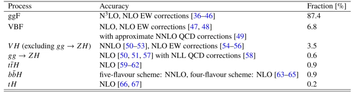
Table 2: Description of cross section predictions used to normalise the MC signal samples, the accuracy of the calculations (in QCD if not noted otherwise), and the contribution of the production modes in the SM. N³LO is the abbreviation for next-to-next-to-next-to-leading order.

Process Accuracy Fraction [%]

ggF N³LO, NLO EW corrections [36–46] 87.4

VBF NLO, NLO EW corrections [47,48] 6.8

with approximate NNLO QCD corrections [49]

V H (excludinggg→Z H) NNLO [50–53], NLO EW corrections [54–56] 3.5

gg→Z H NLO [50,51,57] with NLL QCD corrections [58] 0.6

tt H¯ NLO [59–62] 0.9

bbH¯ five-flavour scheme: NNLO, four-flavour scheme: NLO [63–65] 0.9

t H NLO [66,67] 0.2

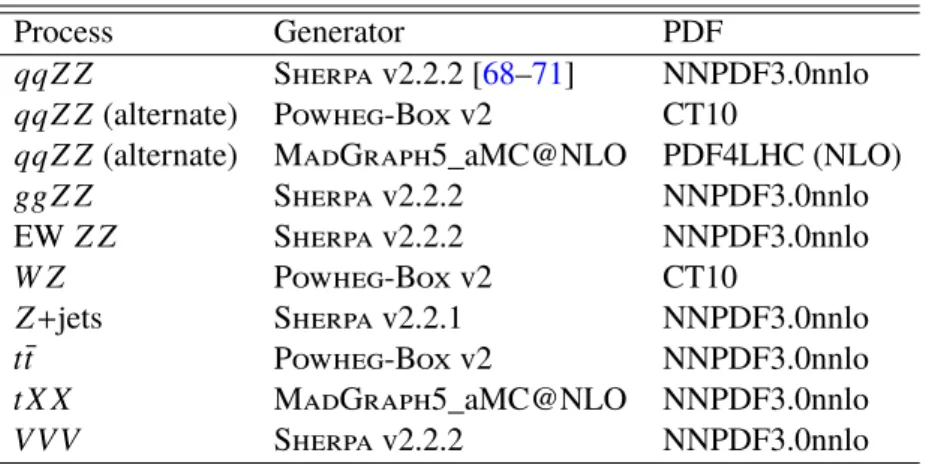
The modelling of the Z Z^∗continuum background (quark-initiated (qqZ Z), gluon-initiated (ggZ Z), and vector boson scattering (EW Z Z) production of Z Z^∗), secondary backgrounds fromW Zproduction, Z bosons produced in association with jets, andt¯tevents, and also the small backgrounds originating from production processes with three electroweak bosons, or at¯tpair and one or more top quarks or electroweak bosons (referred to asV V V andt X X respectively), are also described in Ref. [16]. Some details are given in Table3below. The alternateqqZ Z samples are used for systematic uncertainty studies. Most background processes use Pythia 8 and the A14 set of tuned parameters for decays, parton showers, hardronization, and underlying event.W ZandqqZ Zsimulated with Powheg-Box v2 use the AZNLO set of tuned parameters instead. All processes use EvtGen v1.2.0 for heavy-flavour decays.

Generated events are processed through the ATLAS detector simulation [72] within the Geant4 framework [73] and reconstructed in the same way as collision data. Additionalppinteractions in the same and nearby bunch crossings, referred to as pile-up, are included in the simulation. The pile-up events are generated using PYTHIA 8 with the A3 set of tuned parameters [74] and the NNPDF2.3LO PDF set [75]. The simulated samples are weighted to reproduce the observed distribution of the mean number of interactions per bunch crossing in the data.

Table 3: Description of the production of simulated background samples.

Process Generator PDF

qqZ Z Sherpa v2.2.2 [68–71] NNPDF3.0nnlo qqZ Z (alternate) Powheg-Box v2 CT10

qqZ Z (alternate) MadGraph5_aMC@NLO PDF4LHC (NLO)

ggZ Z Sherpa v2.2.2 NNPDF3.0nnlo

EWZ Z Sherpa v2.2.2 NNPDF3.0nnlo

W Z Powheg-Box v2 CT10

Z+jets Sherpa v2.2.1 NNPDF3.0nnlo

t¯t Powheg-Box v2 NNPDF3.0nnlo

t X X MadGraph5_aMC@NLO NNPDF3.0nnlo

V V V Sherpa v2.2.2 NNPDF3.0nnlo

4 Particle Reconstruction and Event Selection

4.1 Muon reconstruction, identification and calibration

Muon candidate reconstruction within|η| <2.5 is primarily performed by a global fit of reconstructed tracks in the ID and the MS. In the central detector region (|η|<0.1), which has a reduced MS geometrical coverage, muons are also identified by matching a reconstructed ID track to either an MS track segment (segment-tagged muons) or a calorimetric energy deposit consistent with a minimum-ionising particle (calorimeter-tagged muons). For these two cases, the muon momentum is measured from the ID track alone. In the forward MS region (2.5< |η| < 2.7), outside the ID coverage, MS tracks with hits in the three MS layers are accepted and combined with forward ID tracklets, if they exist (stand-alone muons).

Calorimeter-tagged muons are required to havep_T >15 GeV. For all other muon candidates, the transverse momentum is required to be greater than 5 GeV. At most one calorimeter-tagged or stand-alone muon is allowed per Higgs candidate. Additionally, “loose” identification criteria [76] are applied to reject low-quality tracks that are missing measurements in the MS or have poor agreement between MS and ID tracks. Muons are required to be isolated using both calorimeter-based and track-based isolation variables.

Corrections to the reconstructed momentum are applied in order to precisely match the simulation to data. These corrections to the simulated momentum resolution and momentum scale are parameterised as a power expansion in the muonp_T, with each coefficient measured separately for the ID and MS, as a function ofηandφ, from large data samples ofJ/ψ→ µ⁺µ⁻andZ → µ⁺µ⁻decays. The scale corrections range from 0.1% to 0.5% for thep_T of muons originating fromJ/ψ→ µ⁺µ⁻andZ → µ⁺µ⁻decays and account for inaccuracies in the measurement of the energy lost in the traversed material, local magnetic field inaccuracies and geometrical distortions. The corrections to the momentum resolution for muons from J/ψ →µ⁺µ⁻andZ → µ⁺µ⁻are at the percent level. The main sources of systematic uncertainty from these corrections arise from the method used to extract the momentum scale factors and the consistency of the corrections obtained fromJ/ψ →µ⁺µ⁻andZ →µ⁺µ⁻decays. For muons fromZ →µ⁺µ⁻decays, with momenta of about 45 GeV, the momentum scale is determined with a precision of better than 0.05%

for muons with|η| <2, increasing up to about 0.2% for muons with|η| ≥2. The resolution is known with a precision of better than 2% for muons with|η| <1, increasing up to around 10% for muons at the highest ηvalues [76].

After detector alignment, there are residual local misalignments that bias the muon track sagitta, leaving the track χ² invariant [77,78], and introduce a small charge-dependent momentum bias. The bias in the measured momentum of each muon is corrected by an iterative procedure derived fromZ → µ⁺µ⁻ decays [9]. This correction gives a relative improvement of the resolution of the dimuon invariant mass in Zboson decays of about 1%. The systematic uncertainty associated with this correction is estimated for each muon using simulation and is found to be about 0.04% for the average momentum of muons from Z →µ⁺µ⁻decays.

4.2 Electron reconstruction, identification and calibration

Reconstructed electrons are defined as objects consisting of a cluster built from energy deposits in the calorimeter and a matched ID track [79]. The sliding-window algorithm previously exploited in ATLAS for the reconstruction of fixed-size clusters of calorimeter cells [80–82] has been replaced by one employing dynamic, variable-size clusters [79]. Electron ID tracks are fitted using an optimised Gaussian-sum filter (GSF) [81] that accounts for non-linear effects arising from bremsstrahlung energy loss. Quality criteria are used to improve the purity of selected electron objects. The inputs to the likelihood used to evaluate the quality of an electron candidate include measurements from the tracking system, the calorimeter system, and quantities that combine both tracking and calorimeter information. A detailed description is given in Ref. [81]. Electrons are required to be isolated using both the calorimeter-based and track-based isolation variables as described in Ref. [79].

The energy calibration of electrons closely follows the procedure used in Ref. [82], updated for the new energy reconstruction as described in Ref. [79]. The energy of electrons is computed from the energy of the reconstructed cluster using a combination of simulation-based and data-driven corrections. A single simulation-based correction correction, which accounts for the energy lost in the material upstream of the calorimeter, for the energy deposited in the cells neighbouring the cluster inηandφ, and for the energy lost beyond the LAr calorimeter, is computed using multivariate regression algorithms Data driven corrections account for, amongst others, effects related to the material budget in front of the EM calorimeter and material between the presampler and the calorimeter, and the inter-calibration of the different calorimeter layers. The remaining difference in energy scale between data and simulation is defined asα_i, wherei corresponds to different regions inη. Similarly, the mismodelling of the energy resolution is parameterised as anη-dependent additional constant term,c_i. The corresponding energy scale correction is applied to the data, and the resolution correction is applied to the simulation as follows:

E^data,corr =E^data/(1+α_i), σ_E E

_MC,corr

= σ_E E

_MC

⊕c_i, where the symbol⊕denotes a sum in quadrature.

The main sources of systematic uncertainties on the electron energy scale include uncertainties in the method used to extract the energy scale correction factors, as well as uncertainties due to the extrapolation of the energy scale fromZ → e⁺e⁻events to electrons with energies different from those produced in Z →e⁺e⁻decays. The latter arise from the uncertainties in the linearity of the response due to the relative calibration of the different gains used in the calorimeter readout, in the knowledge of the material in front of the calorimeter and material between the presampler and the calorimeter, in the inter-calibration of the different calorimeter layers and in the modelling of the lateral shower shapes. In the case of electrons withE_Taround 40 GeV, the total uncertainty ranges between 0.04% and 0.2% for most of the detector acceptance. For electrons withE_Taround 10 GeV the uncertainty ranges between 0.3% and 0.8%.

Systematic uncertainties in the calorimeter energy resolution arise from uncertainties in the modelling of the sampling term and in the measurement of the constant term inZ boson decays, in the amount of material in front of the calorimeter, and in the modelling of the contribution to the resolution due to fluctuations in the pile-up from additional proton–proton interactions in the same or neighbouring bunch crossings. The uncertainty of the energy resolution for electrons with transverse energy between 30 and 60 GeV varies between 5% and 10%.

4.3 Event selection

Events are required to contain at least four isolated leptons (`=e, µ) that emerge from a common vertex and form two pairs of oppositely charged same-flavour leptons. Electrons are required to be within the full pseudorapidity range of the inner tracking detector (|η| < 2.47) and have transverse energyE_T >7 GeV, while muons are required to be within the pseudorapidity range of the muon spectrometer (|η| < 2.7) and have transverse momentump_T >5 GeV. The three higher-p_T(E_T) leptons in each quadruplet are required to pass thresholds of 20, 15, and 10 GeV, respectively. A detailed description of the event selection can be found in Ref. [16].

The lepton pair with an invariant mass closest to theZ boson mass in each quadruplet is referred to as the leading dilepton, while the remaining pair is referred to as the subleading dilepton. The selected quadruplets are split according to the flavour of the leading and subleading pairs; in decreasing order of expected selection efficiency and resolution, they are 4µ, 2e2µ, 2µ2e, and 4e. Only one quadruplet is selected from each event, based on the mass of the leading dilepton, the final state, and potentially the matrix element value, as described in Ref. [16]. Final-state radiation (FSR) photons are searched for in all events following the procedure described in Ref. [16]. FSR candidates are defined as collinear if they have∆R<0.15 to the nearest lepton in the quadruplet, and non-collinear otherwise. Collinear FSR candidates are considered only for muons from the leading lepton pair, while non-collinear FSR candidates are considered for both muons and electrons from leading and sub-leading Z bosons. Only one FSR candidate is included in the quadruplet with preference given to collinear FSR and to the candidate with the highestp_T. FSR photons are found in 4% of the events and their energy is included in the mass computation, improving them_{4`</sub> resolution by about 1%. In addition, a kinematic fit is performed to constrain the invariant mass of the leading lepton pair to theZ boson mass, improving them<sub>4`}resolution by about 17% [7].

In the range of 115<m_4` <130 GeV, 314 candidate events are observed. The yield is in agreement with an expectation of 316±14 events, 66% of which are expected to be from the signal, assumingm_H =125 GeV.

The observed and expectedm_4`distributions are shown in Figure1.

The dominant contribution to the background is non-resonantZ Z^∗production accounting for∼89% of the total background yield. Events with hadrons or hadron decay products misidentified as prompt leptons, from Z+jets,t¯t, andW Z processes (referred to as the reducible background), contribute ∼9%. V V V andt X X events are estimated to contribute∼2% of the total background. The residual combinatorial background, originating from events with additional prompt leptons, is found to be negligible [16].

4.4 Signal-background discriminant

The transverse momentum and pseudorapidity of the four-lepton system are used together with a matrix- element-based kinematic discriminantD_{Z Z}^∗[83] as inputs to a boosted decision tree (BDT) to discriminate theH →Z Z^∗→4`signal from theZ Z<sup>∗</sup>→4`background. D_{Z Z}^∗ is defined as ln(|M_{H Z Z}^∗|²/|M_{Z Z}^∗|²)

80 100 120 140 160 [GeV]

m4l

0 20 40 60 80 100 120 140 160 180

Events/2.5 GeV

Data Higgs (125 GeV) Z(Z*) tXX, VVV

t Z+jets, t Uncertainty

ATLAS Preliminary

→ 4l ZZ*

→

H -1

= 13 TeV, 139 fb s

Figure 1: The measuredm_4`distribution in data (black points) is shown compared to the expectation, taken from MC simulation for signal,Z Z^∗andZ →4l(Z(Z^∗)in the legend), and tXX and VVV, and from the data-driven estimate (see Sec.5) forZ+jets andtt¯. The uncertainty band includes the statistical and systematic uncertainties on the expectation.

whereM_{H Z Z}^∗ denotes the matrix element for leading-order gluon-fusion-mediatedH → Z Z^∗ → 4` production andM<sub>Z Z</sub><sup>∗</sup> the sum of the corresponding matrix elements for theqq¯ →Z Z<sup>∗</sup>andgg→Z Z<sup>∗</sup> continuum backgrounds, all calculated with MadGraph5 [84]. No cut on the value of the BDT output is applied, but the events are categorised in four exclusive equal-size BDT bins in order to better separate the signal from the background contribution in them<sub>H</sub> fit. Even-sized bins are used as studies showed no significant benefit from attempting to optimise the binning for maximal background rejection. This procedure improves the precision of them<sub>H</sub>measurement in theH →Z Z<sup>∗</sup>→4`decay channel by about 2%. The final analysis is performed in 16 categories, consisting of the four BDT bins for each of the four four-lepton final states.

5 Signal and background model

The measured Higgs bosonm_{4`</sub>distribution is the result of the convolution of its theoretical lineshape, a narrow relativistic Breit–Wigner (BW) distribution of 4.1 MeV width [85] centred onm<sub>H</sub>, with the detector response for the four-lepton invariant mass distribution. The BW width is∼ 2.5 orders of magnitude smaller than them<sub>4`}detector resolution. Therefore, the signal lineshape inm_4`is completely dominated by the detector response.

In this note, them_4` line shape in each analysis category is described with a double-sided Crystal Ball

(DCB [86,87]) probability density function (pdf) consisting of a Gaussian core and two power-law tails:

DC B(m₄`;µ, σ, α₁,n₁, α₂,n₂) =C



















 _n

α1₁

n₁

·e⁻

α2 1 2 ·_n

α1₁−α₁− ^m4`_σ^−µ−n₁

, _m4`−µ

σ

<−α₁ e^−0.5

(m4`−µ)2

σ2 , −α₁≤ _m4`−µ

σ

≤ α_{2 n}

α2₂

n₂

·e⁻

α2 2 2 · _n

α2₂ −α₂+ ^m4`_σ^−µ−n₂

, α₂< _m4`−µ

σ

(1)

where µandσare the mean and standard deviation of the Gaussian core, respectively, then₁,n₂are the exponents of the two power law tails, theα₁,α₂indicate where the power law tails begin, andC is the normalization factor. This approach replaces the Gaussian mixture employed in the most recent ATLAS publication [9].

The value of µis parametrised as a function ofm_H:

µ=a^µ(m_H−125 GeV)+b^µ+125 GeV. (2) This particular form is employed in order to reduce the impact of the error ofa^µonµand to decorrelate the uncertainties ona^µandb^µ. Thea^µ parameters are within a few percent of one for all final states, while the value ofb^µranges from -0.08 GeV in the 2e2µfinal state to -0.31 GeV in the 2µ2efinal state.

The DCB is expanded to use the event-level resolutionσirather than the average resolutionσ. In this case the DCB conditional to the per-event resolution becomes:

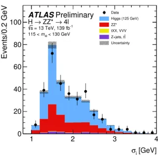
DC B(m₄`;µ, κ×σi, α₁,n₁, α₂,n₂|σi). (3) whereκacts as a calibration constant for the per-event resolution absorbing data-MC differences. In order to estimate the per-eventσ_i, a quantile regression neural network (QRNN) architecture is employed. The QRNN is trained on signal MC events using the Tensorflow library [88] and the Keras Python API [89], for a different target quantile in each final state. The leptonp_T,η, andφ, as well as the constrained four-lepton momentum and its uncertainty, obtained by propagating the individual lepton momentum uncertainties, are used as inputs. The observed and expectedσ_idistributions are shown in Figure2.

The nominal parameters of the signal model for each of the sixteen analysis categories are derived by a simultaneous maximum-likelihood fit on signal MC samples form_H values ranging from 123 GeV to 127 GeV. The resulting pdf is shown in Figure3for them_H =125 GeV signal sample. The non-closure for the derived model, estimated by pseudo-experiments sampling MC events, is at the level of 6 MeVand is treated as an additional systematic uncertainty. When determining the mass in datam_H can vary freely while the other parameters (κ,α_i,n_i,a^µ andb^µ) vary in accordance with the relevant scale and shape systematic uncertainties.

The pdfs for the Z Z^∗andt X X +V V V backgrounds are estimated for each analysis category from MC simulation. The pdf of the reducible background in each analysis category is obtained by summing each component. The components are estimated from MC simulation with the exception of that arising from Z+jet events in which hadrons are misidentified as electrons, for which data from a control region are used [90]. The pdfs are smoothed using an adaptive kernel estimation technique, with Gaussian kernels [91], to reduce statistical fluctuations. The effects of uncertainties that modify the pdfs’ shapes are described by interpolating between the nominal pdfs and pdfs accounting for the relevant systematic variations [92].

Such uncertainties include the theoretical and experimental uncertainties for theZ Z^∗andt X X +V V V pdfs and the knowledge of the relative background composition for the reducible background pdf.

1 2 3 4 [GeV]

σi

0 20 40 60 80 100

Events/0.2 GeV

Data Higgs (125 GeV) ZZ*

tXX, VVV t Z+jets, t Uncertainty

ATLASPreliminary 4l

ZZ* → H →

= 13 TeV, 139 fb-1

s

< 130 GeV m4l

115 <

Figure 2: The event-level resolution σ_i values predicted by the neural network for data (black points) in the 115−130 GeVm_4`range are shown compared to the expectation. The expectation comes from MC simulation for signal,Z Z^∗, and tXX and VVV; forZ+jets andtt¯the shape from MC is normalised using the data-driven estimate.

The uncertainty band includes the statistical and systematic uncertainties on the expectation.

[GeV]

m4l

105 110 115 120 125 130 135 140 ]-1 [GeV 4ldmdN N1

0 0.05 0.1 0.15 0.2 0.25

=125 GeV mH

MC for Higgs

=125 GeV mH

PDF for

ATLASSimulation Preliminary 4l

ZZ* → H →

= 13 TeV s

Figure 3: The pdf derived from signal MC simulation using the per-event resolution (red line) is shown compared to the expectedm_4`distribution in signal MC simulation (black points) form_H=125 GeV. Both the pdf and the MC simulation are normalised to unity.

Them_4`distribution is described by the sum of a signal distribution and the distributions of the backgrounds.

To reduce model dependence, the normalisation of the signal (Z Z^∗ background) pdf in each analysis category is expressed as the product of a signal (background) normalisation modifier per BDT bin, which is allowed to float for a total of eight free normalisation parameters, and the MC expectation for the signal

(background) in that category. The normalisation of the reducible background is constrained based on estimates made from data using minimal input from simulation following the methodology described in Ref. [16]. The normalisation of thet X X+V V V background is constrained according to the uncertainties in the theory prediction.

6 Results

The mass measurement is based on maximising the profile likelihood ratio [93,94]

λ(mH) = L m_H,θ(ˆˆ m_H)

L mˆ_H,θˆ , (4)

where ˆm_Hand ˆθdenote the unconditional-maximum likelihood estimates of the parameters of the likelihood functionL, whileθˆˆis the conditional maximum-likelihood estimate of the parametersθfor a fixed value of the parameter of interestm_H. Systematic uncertainties and their correlations are modelled by introducing nuisance parametersθdescribed by Gaussian or log-normal functions associated with the estimate of the corresponding effect.

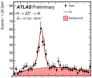
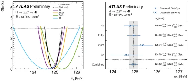
The estimate ofm_His extracted by performing a simultaneous profile likelihood fit to the sixteen analysis categories. The free parameters of the fit arem_H, the normalisation modifiers in each BDT category for the signal andZ Z^∗background (defined in Section5), and the nuisance parameters associated with systematic uncertainties. The measured value ofm_Hwhen accounting for the per-event resolution is found to bem^{Z Z}_H ^∗ =124.92±0.19(stat)₋^+0.09

0.06 (syst) GeV = 124.92⁺⁰₋₀^._.²¹₂₀GeV. Figure4shows the inclusivem<sub>4`</sub> distribution of the data together with the result of the fit to theH→ Z Z<sup>∗</sup>→4`candidates.

[GeV]

4l

m

105 110 115 120 125 130 135 140 145 150 155 160

Events / 1.25 GeV

0 10 20 30 40 50 60 70 80

90 ^Data

Fit Background

ATLASPreliminary 4l

ZZ* → H →

= 13 TeV, 139 fb-1

s

Figure 4: Them_4`data distribution from all categories combined (black points) is shown along with the fit result when accounting for the per-event resolution (red line). The background component of the fit result is shown separately in solid red.

The fit is also performed independently for each decay channel, fitting all BDT categories simultaneously;

the resulting likelihood profiles and results are compared with the combined fit in Figure 5. Results from each category are compatible with each other and the combined result.

[GeV]

mH

124 125 126

)λ-2ln(

0 1 2 3 4 5

6 ^{CombinedStat. only}_4µ

µ 2e2

2e µ 2 4e

ATLASPreliminary 4l

→ ZZ*

→ H

= 13 TeV, 139 fb-1

s

σ 1

σ 2

[GeV]

mH

124 125 126 127

Combined 4e µ2e 2

µ 2e2

µ 4

ATLAS Preliminary

→ 4l ZZ*

→ H

= 13 TeV, 139 fb-1

s

[GeV]

mH

(Sys.)

-0.06 +0.09

(Stat.)

-0.19 +0.19

124.92

(Sys.)

-0.09 +0.10

(Stat.)

-0.74 +0.74

124.59

(Sys.)

-0.10 +0.07

(Stat.)

-0.47 +0.46

125.34

(Sys.)

-0.04 +0.06

(Stat.)

-0.29 +0.29

124.95

(Sys.)

-0.09 +0.13

(Stat.)

-0.28 +0.29

124.80 [GeV]

mH

(Sys.)

-0.06 +0.09

(Stat.)

-0.19 +0.19

124.92

(Sys.)

-0.09 +0.10

(Stat.)

-0.74 +0.74

124.59

(Sys.)

-0.10 +0.07

(Stat.)

-0.47 +0.46

125.34

(Sys.)

-0.04 +0.06

(Stat.)

-0.29 +0.29

124.95

(Sys.)

-0.09 +0.13

(Stat.)

-0.28 +0.29

124.80

Observed: Stat+Sys Observed: Sys-Only

Figure 5: On the left, likelihood scans are shown for the fit in each of the final states 4µ(purple), 2e2µ(orange), 2µ2e (green), and 4e(blue), and combined (black), both with (solid lines) and without (dashed lines) taking systematic uncertainties into account. The horizontal dashed lines indicate the location of the one and twoσuncertainties. On the right, the fit results obtained in each final state are shown together with the combined result. The uncertainty on each point is the total statistical and systematic uncertainty; the brackets show the systematic uncertainty only. The vertical dashed line indicates the combined result, and the grey band its total uncertainty.

The statistical uncertainty ofm_H is estimated by fixing all nuisance parameters to their best-fit values, leaving all remaining parameters unconstrained. The upper bound on the total systematic uncertainty is estimated by subtracting in quadrature the statistical uncertainty from the total uncertainty. The total uncertainty is in agreement with the expectation of 0.19 GeV and is dominated by the statistical component.

Table4shows the impact of the leading systematic uncertainties onm_H. The uncertainties on the muon momentum scale and resolution and the sagitta bias correction, and the electron energy scale, are described in Sections4.1and 4.2respectively. Other sources (including background modelling and simulation statistics) are smaller than 10 MeV.

Table 4: Impact of the leading systematic uncertainties onmH. Systematic Uncertainty Impact (GeV) Muon momentum scale +0.08,−0.06

Electron energy scale ±0.02 Muon momentum resolution ±0.01 Muon sagitta bias correction ±0.01

When the per-event resolution is not used the total uncertainty is found to be⁺⁰₋₀^._.²²₂₁GeV, larger by about 10 MeV than when accounting for the per-event resolution. The observed change in them_Hestimate when not accounting for the per-event resolution is found to be 0.05 GeV: the two estimates agree with ap-value of 26%. Figure6shows the distribution of the expected uncertainty onm_Hobtained from fitting to a set

of pseudo-experiments performed assumingm_H =125 GeV. The 1-sided p-value of the compatibility between the observed and expected uncertainties is found to be 0.17.

[MeV]

mH

Total Uncertainty on

160 180 200 220 240

Arbitrary Units

0 10 20 30 40 50 60 70

3

10−

×

) Expected: 0.20 GeV P(m4l

) Observed: 0.22 GeV P(m4l

) Expected: 0.19 GeV σi

| 4l P(m

) Observed: 0.21 GeV i

| σ P(m4l

ATLASPreliminary 4l

ZZ* → H →

= 13 TeV, 139 fb-1

s

Figure 6: The distributions of the totalm_H uncertainty from pseudo-experiments assumingm_H =125 GeV are shown, for both when the fit does (black) and does not (blue) account for the per-event resolution. The solid lines correspond to the expected uncertainty distribution from the pseudo-experiments while the vertical dashed lines indicate the observed values of the uncertainties.

7 Summary

The mass of the Higgs boson has been measured from a fit to the invariant mass and the predicted invariant mass resolution of the H → Z Z^∗ → 4` decay channel. The results are obtained from the full Run 2 ppcollision data sample recorded by the ATLAS experiment at the CERN Large Hadron Collider at a centre-of-mass energy of 13 TeV, corresponding to an integrated luminosity of 139 fb⁻¹. The measurement is based on the latest calibrations of muons and electrons, and on improvements to the analysis techniques used to obtain the previous result using data collected by ATLAS in 2015 and 2016 .

The measured value of the Higgs boson mass for theH →Z Z^∗→4`channel is m_H =124.92⁺⁰−0^..²¹20GeV.

This result is in good agreement with previous measurements performed by the ATLAS and CMS collaborations.

Appendix

80 100 120 140 160

[GeV]

m4l

0 20 40 60 80 100

Events/2.5 GeV

Data Higgs (125 GeV) Z(Z*) tXX, VVV

t Z+jets, t Uncertainty

ATLAS Preliminary µ

→ 4 ZZ*

→ H

= 13 TeV, 139 fb-1 s

(a)

80 100 120 140 160

[GeV]

m4l

0 10 20 30 40 50

Events/2.5 GeV

Data Higgs (125 GeV) Z(Z*) tXX, VVV

t Z+jets, t Uncertainty

ATLAS Preliminary µ

→ 2e2 ZZ*

→ H

= 13 TeV, 139 fb-1 s

(b)

80 100 120 140 160

[GeV]

m4l

0 5 10 15 20 25

Events/2.5 GeV

Data Higgs (125 GeV) Z(Z*) tXX, VVV

t Z+jets, t Uncertainty

ATLAS Preliminary

→ 4e ZZ*

→

H s = 13 TeV, 139 fb-1

(c)

80 100 120 140 160

[GeV]

m4l

0 5 10 15 20 25 30

Events/2.5 GeV

Data Higgs (125 GeV) Z(Z*) tXX, VVV

t Z+jets, t Uncertainty

ATLAS Preliminary µ2e

→ 2 ZZ*

→

H s = 13 TeV, 139 fb-1

(d)

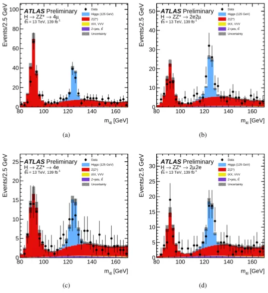
Figure 7: The measuredm_4`distribution in data (black points) is shown compared to the expectation in the (a) 4µ, (b) 2e2µ, (c) 4e, and (d) 2µ2efinal states. The prediction comes from MC simulation for signal, Z Z^∗andZ→4l (Z(Z^∗)in the legend), and tXX and VVV, and from the data-driven estimate forZ+jets andt¯t. The uncertainty band includes all systematic uncertainties.

1 2 3 4 [GeV]

σi

0 10 20 30 40 50 60 70 80

Events/0.2 GeV

Data Higgs (125 GeV) ZZ*

tXX, VVV t Z+jets, t Uncertainty

ATLASPreliminary 4l ZZ* → H →

= 13 TeV, 139 fb-1 s

< 130 GeV m4l 115 <

(a)

1 2 3 4

[GeV]

σi

0 10 20 30 40 50

Events/0.2 GeV

Data Higgs (125 GeV) ZZ*

tXX, VVV t Z+jets, t Uncertainty

ATLASPreliminary 4l ZZ* → H →

= 13 TeV, 139 fb-1 s

< 130 GeV m4l 115 <

(b)

1 2 3 4

[GeV]

σi

0 2 4 6 8 10 12 14 16 18

Events/0.2 GeV

Data Higgs (125 GeV) ZZ*

tXX, VVV t Z+jets, t Uncertainty

ATLASPreliminary 4l ZZ* → H →

= 13 TeV, 139 fb-1 s

< 130 GeV m4l 115 <

(c)

1 2 3 4

[GeV]

σi

0 5 10 15 20 25 30 35 40

Events/0.2 GeV

Data Higgs (125 GeV) ZZ*

tXX, VVV t Z+jets, t Uncertainty

ATLASPreliminary 4l ZZ* → H →

= 13 TeV, 139 fb-1 s

< 130 GeV m4l 115 <

(d)

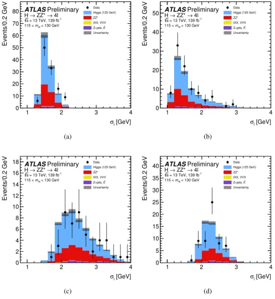
Figure 8: Theσ_i values predicted by the neural network for data (black points) in the 115−130 GeVm_4`range are shown compared to the expectation in the (a) 4µ, (b) 2e2µ, (c) 4e, and (d) 2e2µfinal states. The expectation comes from MC simulation for signal,Z Z^∗, and tXX and VVV; forZ+jets andtt¯the shape from MC simulation is normalised using the data-driven estimate. The uncertainty band includes all systematic uncertainties.

[GeV]

m4l

110 120 130 140 150 160 [GeV]iσ

1.2 1.4 1.6 1.8 2 2.2 2.4

2.6 ^Data

Signal Background

4µ ZZ → H →

= 13 TeV, 139 fb-1 s

ATLASPreliminary

(a)

[GeV]

m4l

110 120 130 140 150 160 [GeV]iσ

1 1.5

2 2.5 3

3.5 ^Data_Signal

Background

2e2µ ZZ → H →

= 13 TeV, 139 fb-1 s

ATLASPreliminary

(b)

[GeV]

m4l

110 120 130 140 150 160 [GeV]iσ

1 1.5

2 2.5 3 3.5 4 4.5

5 Data

Signal Background

4e ZZ → H →

= 13 TeV, 139 fb-1 s

ATLASPreliminary

(c)

[GeV]

m4l

110 120 130 140 150 160 [GeV]iσ

1.6 1.8 2 2.2 2.4 2.6 2.8 3 3.2 3.4 3.6

3.8 ^Data

Signal Background

2e 2µ ZZ → H →

= 13 TeV, 139 fb-1 s

ATLASPreliminary

(d)

[GeV]

m4l

110 120 130 140 150 160 [GeV]iσ

1 1.5

2 2.5 3 3.5 4 4.5

5 Data

Signal Background

4l ZZ → H →

= 13 TeV, 139 fb-1 s

ATLASPreliminary

(e)

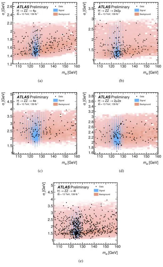
Figure 9: Them_4`vs.σ_idistribution of events is shown in the (a) 4µ, (b) 2e2µ, (c) 4e, and (d) 2µ2efinal states, as well as (e) for all final states combined. The black points are the data, while the signal (background) prediction is in blue (red), with larger boxes (darker colors) indicating a higher abundance. Note that the vertical scale is different between the different final states and the inclusive plot, due to the resolution differences.

[GeV]

4l

m 105 110 115 120 125 130 135 140 145 150 155 160

Events / 2.5 GeV

0 10 20 30 40 50

60 Data

Fit Background

ATLASPreliminary 4µ ZZ* → H →

= 13 TeV, 139 fb-1 s

(a)

[GeV]

4l

m 105 110 115 120 125 130 135 140 145 150 155 160

Events / 2.5 GeV

0 10 20 30 40

50 Data

Fit Background

ATLASPreliminary 2e2µ ZZ* → H →

= 13 TeV, 139 fb-1 s

(b)

[GeV]

4l

m 105 110 115 120 125 130 135 140 145 150 155 160

Events / 2.5 GeV

0 2 4 6 8 10 12 14 16 18

20 Data

Fit Background

ATLASPreliminary 4e ZZ* → H →

= 13 TeV, 139 fb-1 s

(c)

[GeV]

4l

m 105 110 115 120 125 130 135 140 145 150 155 160

Events / 2.5 GeV

0 5 10 15 20 25 30

Data Fit Background

ATLASPreliminary 2e 2µ ZZ* → H →

= 13 TeV, 139 fb-1 s

(d)

Figure 10: The inclusivem_4`data distribution is shown (black points) compared to the fit result (red line) for the (a) 4µ, (b) 2e2µ, (c) 4e, and (d) 2µ2efinal states. The background prediction from the fit is shown separately in solid pink.

−1 −0.5 0 0.5 1 BDT 0

5 10 15 20 25 30 35 40 45

Events

Data Higgs (125 GeV) ZZ*

tXX, VVV t Z+jets, t Uncertainty

ATLASPreliminary 4µ ZZ* →

H → _-1

= 13 TeV, 139 fb s

< 130 GeV m4l 115 <

(a)

−1 −0.5 0 0.5 1

BDT 0

5 10 15 20 25 30 35 40

Events

Data Higgs (125 GeV) ZZ*

tXX, VVV t Z+jets, t Uncertainty

ATLASPreliminary 2e2µ ZZ* →

H → _-1

= 13 TeV, 139 fb s

< 130 GeV m4l 115 <

(b)

1

− −0.5 0 0.5 1

BDT 0

2 4 6 8 10 12 14 16 18 20

Events

Data Higgs (125 GeV) ZZ*

tXX, VVV t Z+jets, t Uncertainty

ATLASPreliminary 4e ZZ* → H →

= 13 TeV, 139 fb-1 s

< 130 GeV m4l 115 <

(c)

1

− −0.5 0 0.5 1

BDT 0

5 10 15 20 25

Events

Data Higgs (125 GeV) ZZ*

tXX, VVV t Z+jets, t Uncertainty

ATLASPreliminary 2e 2µ ZZ* → H →

= 13 TeV, 139 fb-1 s

< 130 GeV m4l 115 <

(d)

1

− −0.5 0 0.5 1

BDT 0

20 40 60 80

Events100

Data Higgs (125 GeV) ZZ*

tXX, VVV t Z+jets, t Uncertainty

ATLASPreliminary 4l ZZ* →

H → _-1

= 13 TeV, 139 fb s

< 130 GeV m4l 115 <

(e)

Figure 11: The distribution of the signal-background discriminant in data (black points) is shown compared to the expectation in the (a) 4µ, (b) 2e2µ, (c) 4e, and (d) 2µ2efinal states, as well as (e) for all final states combined. The prediction comes from MC simulation for signal,Z Z^∗andZ→4l(Z(Z^∗)in the legend), and tXX and VVV, and from the data-driven estimate forZ+jets andtt¯. The uncertainty band includes all systematic uncertainties. The dashed lines indicate the boundaries of the bins used in the analysis.