Measurements of Higgs boson properties in the diphoton decay channel with 36 fb−

EUROPEAN ORGANISATION FOR NUCLEAR RESEARCH (CERN)

Phys. Rev. D 98 (2018) 052005 DOI: 10.1103/PhysRevD.98.052005

CERN-EP-2017-288 11th January 2019

Measurements of Higgs boson properties in the diphoton decay channel with 36 fb ^{− 1} of p p collision data at √

s = 13 TeV with the ATLAS detector

The ATLAS Collaboration

Properties of the Higgs boson are measured in the two-photon final state using 36 . 1 fb

of proton–proton collision data recorded at

√ s = 13 TeV by the ATLAS experiment at the Large Hadron Collider. Cross-section measurements

for the production of a Higgs boson through gluon–gluon fusion, vector-boson fusion, and in association with a vector boson or a top-quark pair are reported. The signal strength, defined as the ratio of the observed to the expected signal yield, is measured for each of these production processes as well as inclusively. The global signal strength measurement of 0.99 ± 0.14 improves on the precision of the ATLAS measurement at √

s = 7 and 8 TeV by a factor of two. Measurements of gluon–gluon fusion and vector-boson fusion productions yield signal strengths compatible with the Standard Model prediction. Measurements of simplified template cross sections, designed to quantify the different Higgs boson production processes in specific regions of phase space, are reported. The cross section for the production of the Higgs boson decaying to two isolated photons in a fiducial region closely matching the experimental selection of the photons is measured to be 55 ± 10 fb, which is in good agreement with the Standard Model prediction of 64 ± 2 fb. Furthermore, cross sections in fiducial regions enriched in Higgs boson production in vector-boson fusion or in association with large missing transverse momentum, leptons or top-quark pairs are reported. Differential and double-differential measurements are performed for several variables related to the diphoton kinematics as well as the kinematics and multiplicity of the jets produced in association with a Higgs boson. These differential cross sections are sensitive to higher order QCD corrections and properties of the Higgs boson, such as its spin and CP quantum numbers. No significant deviations from a wide array of Standard Model predictions are observed. Finally, the strength and tensor structure of the Higgs boson interactions are investigated using an effective Lagrangian, which introduces additional CP-even and CP-odd interactions. No significant new physics contributions are observed.

© 2019 CERN for the benefit of the ATLAS Collaboration.

arXiv:1802.04146v2 [hep-ex] 10 Jan 2019

Contents

1 Introduction 4

1.1 Higgs boson production-mode cross sections and signal strengths 5

1.2 Simplified template cross sections 5

1.3 Fiducial integrated and differential cross sections 6

2 ATLAS detector 9

3 Data set 10

4 Event simulation 10

5 Event reconstruction and selection 12

5.1 Photon reconstruction and identification 12

5.2 Event selection and selection of the diphoton primary vertex 14 5.3 Reconstruction and selection of hadronic jets, b -jets, leptons and missing transverse

momentum 14

6 Signal and background modeling of diphoton mass spectrum 16

6.1 Signal model 16

6.2 Background composition and model 17

6.3 Statistical model 20

6.4 Limit setting in the absence of a signal 21

7 Systematic uncertainties 22

7.1 Systematic uncertainties in the signal and background modeling from fitting the m

spectrum 22

7.2 Experimental systematic uncertainties affecting the expected event yields 24 7.3 Theoretical and modeling uncertainties for results based on event reconstruction cat-

egories 26

7.4 Theoretical and modeling uncertainties for fiducial integrated and differential results 27 7.5 Illustration of model errors for simplified template cross section and fiducial cross

section measurements 28

8 Measurement of total production-mode cross sections, signal strengths, and simplified

template cross sections 29

8.1 Event categorization 29

8.1.1 t¯ tH and tH enriched categories 29

8.1.2 V H leptonic enriched categories 30

8.1.3 BSM enriched and V H hadronic categories 31

8.1.4 VBF enriched categories 32

8.1.5 Untagged categories 32

8.1.6 Categorization summary 33

8.2 Production mode measurements 38

8.2.1 Observed Data 38

8.2.2 Signal strengths 38

8.2.3 Production-mode cross sections 44

8.2.4 Simplified template cross sections 46

8.2.5 Coupling-strength fits 50

9 Measurement of fiducial integrated and differential cross sections 53 9.1 Particle-level fiducial definition of the Higgs boson diphoton cross sections 53

9.2 Fiducial integrated and differential cross sections 54

9.3 Measurements of cross sections of fiducial integrated regions 56 9.4 Measurements of cross sections of inclusive and exclusive jet multiplicities 62 9.5 Measurements of differential and double-differential cross sections 63 9.5.1 Measurements of cross sections probing the Higgs boson production kinematics 63 9.5.2 Measurements of cross sections probing the jet kinematics 65 9.5.3 Measurements of cross sections probing spin and CP 66

9.5.4 Cross sections probing the VBF production mode 68

9.5.5 Double-differential cross sections 69

9.5.6 Impact of systematic uncertainties on results 69

9.5.7 Compatibility of measured distributions with the Standard Model 73 9.5.8 Search for anomalous Higgs-boson interactions using an effective field theory

approach 75

10 Summary and conclusions 80

Appendix 84

A Simplified template cross-section framework 84

B Minimally merged simplified template cross sections 87

C Additional unfolded differential cross sections 90

D Diphoton acceptance, photon isolation and non-perturbative correction factors for

parton-level gluon–gluon fusion calculations 90

E Supplement to event categorization 91

F Limits on µ

and µ

using pseudo-experiments 102

G Summary of couplings results 102

G.1 Signal strengths 102

G.2 Production mode cross sections 103

G.3 Simplified template cross sections 103

G.4 Minimally merged simplified template cross sections 104

H Observed and expected correlation maps 105

1 Introduction

In July 2012, the ATLAS [1] and CMS [2] experiments announced the discovery of a Higgs boson [3, 4] using proton–proton collisions collected at center-of-mass energies

√ s = 7 TeV and 8 TeV at the CERN Large Hadron Collider (LHC). Subsequent measurements of its properties were found to be consistent with those expected for the Standard Model (SM) Higgs boson [5] with a mass m

= 125 . 09 ± 0 . 21 ( stat . ) ± 0 . 11 ( syst . ) GeV [6].

Following the modifications of the LHC to provide proton–proton collisions at a center-of-mass energy of

√ s = 13 TeV, the Higgs sector can be probed more deeply: the data set collected in 2015 and 2016 allows inclusive Higgs boson measurements to be repeated with about two times better precision than to those done at

√ s = 7 and 8 TeV with the Run 1 data set. The increased center-of- mass energy results in much larger cross sections for events at high partonic center-of-mass energy.

This implies improved sensitivity to a variety of interesting physics processes, such as Higgs bosons produced at high transverse momentum or Higgs bosons produced in association with a top–antitop quark pair. The Higgs boson decay into two photons ( H → γγ ) is a particularly attractive way to study the properties of the Higgs boson and to search for deviations from the Standard Model predictions due to beyond-Standard Model (BSM) processes. Despite the small branching ratio, ( 2 . 27 ± 0 . 07 ) × 10

³ for m

= 125 . 09 GeV [7], a reasonably large signal yield can be obtained thanks to the high photon reconstruction and identification efficiency at the ATLAS experiment. Furthermore, due to the excellent photon energy resolution of the ATLAS calorimeter, the signal manifests itself as a narrow peak in the diphoton invariant mass ( m

) spectrum on top of a smoothly falling background, and the Higgs boson signal yield can be measured using an appropriate fit to the m

distribution of the selected events.

In this paper, the results of measurements of the Higgs boson properties in the diphoton decay channel are presented using 36 . 1 fb

¹ of pp collision data collected at

√ s = 13 TeV by the ATLAS detector in 2015 and 2016. All the measurements are performed under the assumption that the Higgs boson mass is 125 . 09 GeV, and are compared to Standard Model predictions. Three types of measurements are presented in this paper and are summarized in the remainder of this section: (i) measurements of the total Higgs boson production-mode cross sections and “signal strengths”; (ii) cross sections using the SM production modes as “templates” in simplified fiducial regions; and (iii) measurements of integrated or differential cross sections in fiducial phase-space regions closely matched to the experimental selection.

The rest of this paper is organized as follows. Section 2 provides a brief description of the ATLAS detector, and Section 3 describes the selected data set. The generation of simulated event samples is described in Section 4. Section 5 gives an overview of the event reconstruction and selection, and Section 6 explains the signal and background modeling used in the measurement. The sources of systematic uncertainties are detailed in Section 7. Section 8 describes the measurement of the total Higgs boson production-mode cross sections, signal strengths, and simplified template cross sections (STXS). Similarly, Section 9 describes the measurement of the fiducial and differential cross sections.

Section 10 concludes with a brief summary of the main findings.

1.1 Higgs boson production-mode cross sections and signal strengths

In this paper, cross sections times branching ratio of the Higgs to two photons B(H → γγ) are measured for inclusive Higgs boson production, as well as for several individual production processes:

gluon–gluon fusion (ggH), vector-boson fusion (VBF), Higgs boson production in association with a vector boson ( V H ), and production of a Higgs boson in association with a top–antitop quark pair ( t tH ¯ ) or a single top quark ( t -channel and W-associated, respectively denoted as tHq and tHW , or in their sum as “ tH ”). In the SM, gluon–gluon fusion is the dominant production mechanism at the LHC, contributing to about 87% of the total cross section at

√ s = 13 TeV [7]. Vector-boson fusion and associated production with either a vector boson, with a top–antitop quark pair or a bottom–antibottom quark pair correspond to 6.8%, 4.0%, 0.9%, and 0.9%, respectively, of the total Higgs boson production cross section.

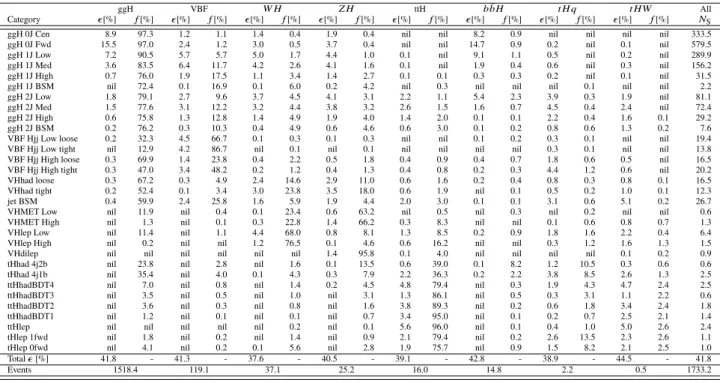
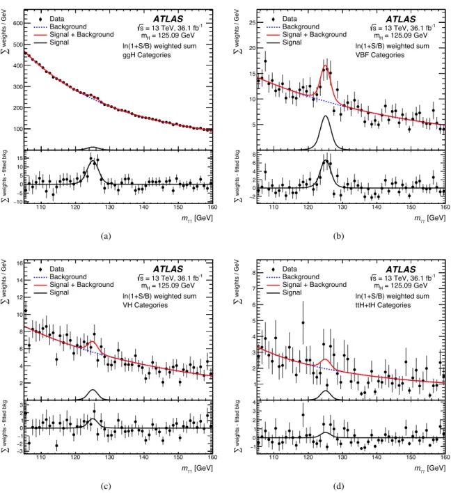
The data are divided into 31 categories based on the reconstructed event properties to maximize the sensitivity to different production modes and the different regions of the simplified template cross sections, which are further described in Section 1.2. The categories are defined using the expected properties of the different production mechanisms: 10 categories aimed to measure gluon–gluon fusion properties, 4 categories to measure vector-boson fusion, 8 categories that target associated production with vector bosons with different final states, and 9 categories that target associated production with a top–antitop quark pair or a single top-quark. The definition of each category was optimized using simulated events and a full summary of the categories can be found in Section 8. In the sequence of the classification, priority is given to categories aimed at selecting signal events from processes with smaller cross sections.

In order to probe the production mechanisms independently of the H → γγ branching ratio, ratios of the different production-mode cross sections normalized to gluon–gluon fusion are also reported, with their full experimental correlations. In addition, measurements of the signal strength µ , which is the ratio of the measured cross section to the SM prediction, are given for the different production processes as well as for the inclusive production. Finally, coupling-strength modifiers, which are scale factors of the tree-level Higgs boson couplings to the different particles or of the effective Higgs boson couplings to photons and gluons from loop-induced processes, are reported.

1.2 Simplified template cross sections

The measurements of cross sections separated by the production mode as presented in the previous section are extended to measurements in specific regions of phase space using the framework of the

“simplified template cross sections” introduced in Refs. [7, 8]. These are reported as cross section times B(H → γγ ) for a Higgs boson absolute rapidity 1 | y

| less than 2.5 and with further particle- level requirements. The different production modes are separated in a theoretically motivated way using the SM modes ggH, VBF, V H and top-quark-associated production modes as “templates”. The fiducial regions are defined in a “simplified” way using the measured kinematics and topology of the

1

The ATLAS experiment uses a right-handed coordinate system with its origin at the nominal interaction point (IP) in the

z x

final state, defined by the Higgs boson, the hadronic jets and the vector bosons or top quarks in the event, to avoid large model-dependent extrapolations. The Higgs boson is treated as a stable final-state particle, which allows an easy combination with other decay channels. Similarly, vector bosons or top quarks are treated as stable particles, but the cases of leptonic and hadronic decays of the vector boson are distinguished.

In this paper a merged version of the so-called “stage-1” simplified template cross-section measure- ments are investigated. These measurements provide more information for theoretical reinterpretation compared to the signal strength measurements used in Run 1 and are defined to reduce the theoretical uncertainties typically folded into the signal strength results. In the full stage-1 proposal, template cross sections would be measured in 31 regions of phase space for | y

| < 2 . 5, where the latter require- ment reflects the experimental acceptance. The experimental categories used in this study (the same as those used for the signal strength measurements) have been optimized to provide the maximum sensitivity to such regions [7, 8].

Since the current data set is not large enough to probe all of the stage-1 cross sections with sufficiently small statistical uncertainties, regions with poor sensitivity or with large anti-correlations are merged together into ten regions: Six regions probe gluon-fusion Higgs boson production with zero, one, and two jets associated with them. Two regions probe VBF Higgs boson production and Higgs boson production associated with vector bosons that decay hadronically. A dedicated cross section is measured for Higgs boson production associated with vector bosons that decay via leptonic modes.

The final cross section measures top-associated ( t tH ¯ and tH ) Higgs-boson production. To retain sensitivity to beyond the Standard Model Higgs boson production , the ≥ 1 jet, p

T > 200 GeV gluon–

gluon fusion and p

T > 200 GeV VBF+ V H regions are not merged with other regions. Here p

T and p

T

denote the Higgs boson and leading jet transverse momenta, respectively, where the leading jet is the highest transverse momentum jet in a given event. However, due to their large anti-correlation, only the cross section for the summed yield of these two regions is quoted here, and thus a total of nine kinematic regions are reported. The experimental sensitivity to the difference in the yields of these two regions is expected to be small, and the corresponding result is treated as a nuisance parameter rather than a measurement.

Table 1 summarizes the ten probes merged stage-1 cross sections and details which of the full 31 stage-1 cross sections were merged (middle and last column). A detailed description of the full 31 cross section proposal can be found in Appendix A.

1.3 Fiducial integrated and differential cross sections

Fiducial integrated and differential cross sections have previously been measured at

√ s = 8 TeV in

the H → γγ decay channel by both the ATLAS [9] and the CMS [10] Collaborations. In this paper,

fiducial cross sections are determined in a variety of phase-space regions sensitive to inclusive Higgs

boson production and to explicit Higgs boson production mechanisms. The measurement of these cross

sections provides an alternative way to study the properties of the Higgs boson and to search for physics

beyond the Standard Model. For each fiducial region of an integrated cross-section measurement or

bin of a differential distribution, the H → γγ signal is extracted using a fit to the corresponding

diphoton invariant mass spectrum. The cross sections are determined by correcting these yields for

experimental inefficiencies and resolution effects, and by taking into account the integrated luminosity

Table 1: The particle-level kinematic regions of the stage-1 simplified template cross sections, along with the intermediate set of regions used for the measurements presented in this paper. All regions require | y

| < 2.5.

Jets are defined using the anti- k

algorithm with radius parameter R = 0.4 and are required to have p

> 30 GeV.

The leading jet and Higgs boson transverse momenta are denoted by p

T

and p

T

, respectively. The transverse momentum of the Higgs boson and the leading and subleading jet is denoted as p

T

with the subleading jet being the second highest momentum jet in a given event. Events are considered “VBF-like” if they contain at least two jets with an invariant mass of m

> 400 GeV and a rapidity separation between the two jets of |∆y

| > 2 . 8. Events are considered “ V H -like” if they contain at least two jets with an invariant mass of 60 GeV < m

< 120 GeV. All qq

→ Hqq

VBF and V H events (with the vector boson V decaying hadronically) which are neither VBF nor V H -like are part of the “Rest” selection. For the p

T

> 200 GeV gluon–gluon fusion and p

T

> 200 GeV VBF + V H regions, only the sum of the corresponding cross sections is reported while the difference of the two is profiled in the fit. In total, the cross sections for nine kinematic regions are measured. The small contributions from b bH ¯ are merged with ggH. The process gg → Z H refers only to box and loop processes dominated by top and bottom quarks (see Section 4 for more details).

Process Measurement region Particle-level stage-1 region

ggH + gg → Z(→ qq)H 0-jet 0-jet

1-jet, p

T

< 60 GeV 1-jet, p

T

< 60 GeV 1-jet, 60 ≤ p

T

< 120 GeV 1-jet, 60 ≤ p

T

< 120 GeV 1-jet, 120 ≤ p

T

< 200 GeV 1-jet, 120 ≤ p

T

< 200 GeV

≥ 1-jet, p

T

> 200 GeV 1-jet, p

T

> 200 GeV

≥ 2-jet, p

T

> 200 GeV

≥ 2-jet, p

T

< 200 GeVor VBF-like ≥ 2-jet, p

T

< 60 GeV

≥ 2-jet, 60 ≤ p

T

< 120 GeV

≥ 2-jet, 120 ≤ p

T

< 200 GeV VBF-like, p

T

< 25 GeV VBF-like, p

T

≥ 25 GeV qq

→ Hqq

(VBF + V H ) p

T

< 200 GeV p

T

< 200 GeV, VBF-like, p

T

< 25 GeV p

T

< 200 GeV, VBF-like, p

T

≥ 25 GeV p

T

< 200 GeV, V H -like p

T

< 200 GeV, Rest p

T

> 200 GeV p

T

> 200 GeV

V H (leptonic decays) V H leptonic q q ¯ → Z H , p

T

< 150 GeV q q ¯ → Z H , 150 < p

T

< 250 GeV, 0-jet q q ¯ → Z H , 150 < p

T

< 250 GeV, ≥ 1-jet q q ¯ → Z H , p

T

> 250 GeV q q ¯ → W H , p

T

< 150 GeV q q ¯ → W H , 150 < p

T

< 250 GeV, 0-jet q q ¯ → W H , 150 < p

T

< 250 GeV, ≥ 1-jet q q ¯ → W H , p

T

> 250 GeV gg → Z H , p

T

< 150 GeV gg → Z H , p

T

> 150 GeV, 0-jet gg → Z H , p

T

> 150 GeV, ≥ 1-jet

Top-associated production top t tH ¯

W -associated tH ( tHW )

of the data. No attempt is made to separate individual production modes in favor of presenting fiducial regions enriched with a given production mode.

The inclusive fiducial region is defined at the particle level by two photons, not originating from the decay of a hadron, that have absolute pseudorapidity |η| < 2 . 37, excluding the region 1 . 37 < |η| <

1 . 52,2 with the leading (subleading) photon transverse momentum greater than 35% (25%) of m

. The two photons are required to be isolated from hadronic activity by imposing that the summed transverse momentum of charged stable particles (with a mean lifetime that satisfies cτ > 10 mm) with p _T > 1 GeV, within a cone of ∆R = 0 . 2 centered on the photon direction, be less than 5% of the photon transverse momentum. This selection is applied to all the presented fiducial integrated and differential cross section results and the isolation criterion was tuned to mimic the detector level selection. One additional cross section and three cross-section limits are reported in smaller fiducial regions sensitive to specific Higgs boson production mechanisms:

• a VBF-enhanced region with two jets with large invariant mass and rapidity separation,

• a region of events containing at least one charged lepton3,

• a region of events with large missing transverse momentum,

• and a region of events with a topology matching the presence of a top–antitop quark pair.

The fiducial cross section for different jet multiplicities are reported and compared to several predic- tions. Eleven fiducial differential cross sections are reported, for events belonging to the inclusive fiducial region as a function of the following observables:

• p

T and |y

| , the transverse momentum and rapidity of the diphoton system,

• p

T and | y

| , the transverse momentum and rapidity of the leading jet,

• p

T and | y

| , the transverse momentum and rapidity of the subleading jet,

• | cos θ

| , the cosine of the angle between the beam axis and the diphoton system in the Collins–

Soper frame [11],

• ∆φ

and |∆ y

| , the difference in azimuthal angle and in rapidity between the leading and subleading jets,

• |∆φ

| , the difference in azimuthal angle between the dijet system formed by the leading and subleading jets and the diphoton system,

• and m

, the invariant mass of the leading and subleading jets.

Seven additional variables are reported in Appendix C. Inclusive Higgs boson production is dominated by gluon–gluon fusion, for which the transverse momentum of the Higgs boson is largely balanced by the emission of soft gluons and quarks. Measuring p

T probes the perturbative QCD modeling of this production mechanism which is mildly sensitive to the bottom and charm quark Yukawa couplings of the Higgs boson [12]. The distribution at high transverse momentum is sensitive to new heavy particles coupling to the Higgs boson and to the top quark Yukawa coupling. The rapidity distribution of the Higgs boson is also sensitive to the modeling of the gluon–gluon fusion production mechanism, as

2

This pseudorapidity interval corresponds to the transition region between the barrel and endcap sections of the ATLAS electromagnetic calorimeter, see Section 2.

3

In this paper reconstructed charged leptons denote electrons and muons.

well as to the parton distribution functions (PDFs) of the colliding protons. The transverse momentum and absolute rapidity of the leading and subleading jets probe the perturbative QCD modeling and are sensitive to the relative contributions of the different Higgs production mechanisms. The angular variables | cos θ

| and ∆ φ

are sensitive to the spin and CP quantum numbers of the Higgs boson. The dijet rapidity separation |∆y

| , the dijet mass m

and the azimuthal difference between the dijet and diphoton system |∆φ

| are sensitive to the VBF production mechanism. All fiducial differential cross sections are reported with their full statistical and experimental correlations and are compared to several predictions.

The strength and tensor structure of the Higgs boson interactions are investigated using an effective Lagrangian, which introduces additional CP-even and CP-odd interactions that can lead to deviations in the kinematic properties and event rates of the Higgs boson and of the associated jets from those in the Standard Model. This is done by a simultaneous fit to five differential cross sections, which are sensitive to the Wilson coefficients of four dimension-six CP-even or CP-odd operators of the Strongly Interacting Light Higgs formulation [13]. A similar analysis was carried out at

√ s = 8 TeV by the ATLAS Collaboration [14].

2 ATLAS detector

The ATLAS detector [1] covers almost the entire solid angle about the proton–proton interaction point. It consists of an inner tracking detector, electromagnetic and hadronic calorimeters, and a muon spectrometer.

Charged-particle tracks and interaction vertices are reconstructed using information from the inner detector (ID). The ID consists of a silicon pixel detector (including the insertable B-layer [15] installed before the start of Run 2), of a silicon microstrip detector, and of a transition radiation tracker (TRT).

The ID is immersed in a 2 T axial magnetic field provided by a thin superconducting solenoid. The silicon detectors provide precision tracking over the pseudorapidity interval |η| < 2 . 5, while the TRT offers additional tracking and substantial discrimination between electrons and charged hadrons for

|η| < 2 . 0.

The solenoid is surrounded by electromagnetic (EM) and hadronic sampling calorimeters allowing

energy measurements of photons, electrons and hadronic jets and discrimination between the different

particle types. The EM calorimeter is a lead/liquid-argon (LAr) sampling calorimeter. It consists of a

barrel section, covering the pseudorapidity region |η| < 1 . 475, and of two endcap sections, covering

1 . 375 < |η| < 3 . 2. The EM calorimeter is divided in three layers, longitudinally in depth, for |η| < 2 . 5,

and in two layers for 2 . 5 < |η| < 3 . 2. In the regions |η| < 1 . 4 and 1 . 5 < |η| < 2 . 4, the first layer has a

fine η segmentation to discriminate isolated photons from neutral hadrons decaying to pairs of close-by

photons. It also allows, together with the information from the cluster barycenter in the second layer,

where most of the energy is collected, a measurement of the shower direction without assumptions

on the photon production point. In the range of |η| < 1 . 8 a presampler layer allows corrections to be

made for energy losses upstream of the calorimeter. The hadronic calorimeter reconstructs hadronic

showers using steel absorbers and scintillator tiles ( |η | < 1 . 7), or either copper (1 . 5 < |η | < 3 . 2) or

A two-level trigger system [16] was used during the

√ s = 13 TeV data-taking period. Dedicated hard- ware implements the first-level (L1) trigger selection, using only a subset of the detector information and reducing the event rate to at most 100 kHz. Events satisfying the L1 requirements are processed by a high-level trigger executing, on a computer farm, algorithms similar to the offline reconstruction software, in order to reduce the event rate to approximately 1 kHz.

3 Data set

Events were selected using a diphoton trigger requiring the presence in the EM calorimeter of two clusters of energy depositions with transverse energy above 35 GeV and 25 GeV for the leading (highest transverse energy) and subleading (second highest transverse energy) cluster. In the high-level trigger the shape of the energy deposition of both clusters was required to be loosely consistent with that expected from an electromagnetic shower initiated by a photon. The diphoton trigger has an efficiency greater than 99% for events that satisfy the final event selection described in Section 5.

After the application of data quality requirements, the data set amounts to an integrated luminosity of 36 . 1 fb

¹ , of which 3.2 fb

¹ were collected in 2015 and 32.9 fb

¹ were collected in 2016. The mean number of proton–proton interactions per bunch crossing is 14 in the 2015 data set and 25 in the 2016 data set.

4 Event simulation

Signal samples were generated for the main Higgs boson production modes using Monte Carlo event generators as described in the following. The mass and width of the Higgs boson were set in the simulation to m

= 125 GeV and Γ

= 4 . 07 MeV [17], respectively. The samples are normalized with the latest available theoretical calculations of the corresponding SM production cross sections, as summarized in Ref. [7] and detailed below. The normalization of all Higgs boson samples also accounts for the H → γγ branching ratio of 0.227% calculated with HDECAY [18, 19] and PROPHECY4F [20–

22].

Higgs boson production via ggH is simulated at next-to-next-to-leading-order (NNLO) accuracy in QCD using the Powheg NNLOPS program [23], with the PDF4LHC15 PDF set [24]. The simulation achieves NNLO accuracy for arbitrary inclusive gg → H observables by reweighting the Higgs boson rapidity spectrum in Hj-MiNLO [25] to that of HNNLO [26]. The transverse momentum spectrum of the Higgs boson obtained with this sample was found to be compatible with the fixed-order HNNLO calculation [26] and the Hres2.3 calculation [27, 28] performing resummation at next-to-next-to- leading-logarithm accuracy matched to a NNLO fixed-order calculation (NNLL+NNLO). The Hres prediction includes the effects of the top and bottom quark masses up to NLO precision in QCD and uses dynamical renormalization ( µ _R ) and factorization ( µ

) scales, µ

= µ _R = 0 . 5

q

m ²

+ p

T

2 . The

parton-level events produced by the Powheg NNLOPS program are passed to Pythia8 [29] to provide

parton showering, hadronization and underlying event, using the AZNLO set of parameters that are

tuned to data [30]. The sample is normalized such that it reproduces the total cross section predicted by

a next-to-next-to-next-to-leading-order (N ³ LO) QCD calculation with NLO electroweak corrections

applied [31–34].

Higgs boson production via VBF is generated at NLO accuracy in QCD using the Powheg-Box program [35–38] with the PDF4LHC15 PDF set. The parton-level events are passed to Pythia8 to provide parton showering, hadronization and the underlying event, using the AZNLO parameter set.

The VBF sample is normalized with an approximate-NNLO QCD cross section with NLO electroweak corrections applied [39–41].

Higgs boson production via V H is generated at NLO accuracy in QCD through qq / qg -initiated production, denoted as q q ¯

→ V H , and through gg → Z H production using Powheg-Box [42] with the PDF4LHC15 PDF set. Higgs boson production through gg → Z H has two distinct sources: a contribution with two additional partons, gg → Z Hq q ¯ , and a contribution without any additional partons in the final state, including box and loop processes dominated by top and bottom quarks. In the following, the gg → Z H notation refers only to this latter contribution. Pythia8 is used for parton showering, hadronization and the underlying event using the AZNLO parameter set. The samples are normalized with cross sections calculated at NNLO in QCD and NLO electroweak corrections for q q ¯

→ V H and at NLO and next-to-leading-logarithm accuracy in QCD for gg → Z H [43–45].

Higgs boson production via t tH ¯ is generated at NLO accuracy in QCD using MG5_aMC@NLO [46]

with the NNPDF3.0 PDF set [47] and interfaced to Pythia8 to provide parton showering, hadronization and the underlying event, using the A14 parameter set [48]. The t tH ¯ sample is normalized with a cross section calculation accurate to NLO in QCD with NLO electroweak corrections applied [49–52].

Higgs boson production via b bH ¯ is simulated using MG5_aMC@NLO [53] interfaced to Pythia8 with the CT10 PDF set [54], and is normalized with the cross-section calculation obtained by matching, using the Santander scheme, the five-flavor scheme cross section accurate to NNLO in QCD with the four-flavor scheme cross section accurate to NLO in QCD [55–57]. The sample includes the effect of interference with the gluon–gluon fusion production mechanism.

Associated production of a Higgs boson with a single top-quark and a W -boson ( tHW ) is generated at NLO accuracy, removing the overlap with the t tH ¯ sample through a diagram regularization technique, using MG5_aMC@NLO interfaced to Herwig++ [58–60], with the Herwig++ UEEE5 parameter set for the underlying event and the CT10 PDF set using the five-flavor scheme. Simulated Higgs boson events in association with a single top-quark, a b -quark and a light quark ( tHq ) are produced at LO accuracy in QCD using MG5_aMC@NLO interfaced to Pythia8 with the CT10 PDF set within the four-flavor scheme and using the A14 parameter set. The tHW and tHq samples are normalized with calculations accurate to NLO in QCD [61].

The generated Higgs boson events are passed through a Geant4 [62] simulation of the ATLAS detector [63] and reconstructed with the same analysis software used for the data.

Background events from continuum γγ production and V γγ production are simulated using the Sherpa event generator [64], with the CT10 PDF set and the Sherpa default parameter set for the underlying-event activity. The corresponding matrix elements for γγ and Vγγ are calculated at leading order (LO) in the strong coupling constant α _S with the real emission of up to three or two additional partons, respectively, and are merged with the Sherpa parton shower [65] using the Meps@lo prescription [66].

γγ

Table 2: Summary of the event generators and PDF sets used to model the signal and the main background processes. The SM cross sections σ for the Higgs production processes with m

= 125 . 09 GeV are also given separately for

√ s = 13 TeV, together with the orders of the calculations corresponding to the quoted cross

sections, which are used to normalize the samples, after multiplication by the Higgs boson branching ratio to diphotons, 0.227%. The following versions were used: Pythia8 version 8.212 (processes) and 8.186 (pile-up overlay); Herwig++ version 2.7.1; Powheg-Box version 2; MG5_aMC@NLO version 2.4.3; Sherpa version 2.2.1

Process Generator Showering PDF set σ [ pb ]

Order of calculation of σ

√ s = 13 TeV

ggH Powheg NNLOPS Pythia8 PDF4LHC15 48.52 N

LO(QCD)+NLO(EW)

VBF Powheg-Box Pythia8 PDF4LHC15 3.78 NNLO(QCD)+NLO(EW)

W H Powheg-Box Pythia8 PDF4LHC15 1.37 NNLO(QCD)+NLO(EW)

q q ¯

→ Z H Powheg-Box Pythia8 PDF4LHC15 0.76 NNLO(QCD)+NLO(EW)

gg → Z H Powheg-Box Pythia8 PDF4LHC15 0.12 NLO+NLL(QCD)

t¯ tH MG5_aMC@NLO Pythia8 NNPDF3.0 0.51 NLO(QCD)+NLO(EW)

b¯ bH MG5_aMC@NLO Pythia8 CT10 0.49 5FS(NNLO)+4FS(NLO)

t -channel tH MG5_aMC@NLO Pythia8 CT10 0.07 4FS(LO)

W -associated tH MG5_aMC@NLO Herwig++ CT10 0.02 5FS(NLO)

γγ Sherpa Sherpa CT10

V γγ Sherpa Sherpa CT10

Additional proton–proton interactions (pileup) are included in the simulation for all generated events such that the average number of interactions per bunch crossing reproduces that observed in the data.

The inelastic proton–proton collisions were produced using Pythia8 with the A2 parameter set [68]

that are tuned to data and the MSTW2008lo PDF set [69]. A summary of the used signal and background samples is shown in Table 2.

5 Event reconstruction and selection

5.1 Photon reconstruction and identification

The reconstruction of photon candidates is seeded by energy clusters in the electromagnetic calorimeter

with a size of ∆η × ∆φ = 0.075 × 0.125, with transverse energy E _T greater than 2.5 GeV [70]. The

reconstruction is designed to separate electron from photon candidates, and to classify the latter

as unconverted or converted photon candidates. Converted photon candidates are associated with

the conversion of photons into electron–positron pairs in the material upstream the electromagnetic

calorimeter. Conversion vertex candidates are reconstructed from either two tracks consistent with

originating from a photon conversion, or one track that does not have any hits in the innermost pixel

layer. These tracks are required to induce transition radiation signals in the TRT consistent with the

electron hypothesis, in order to suppress backgrounds from non-electron tracks. Clusters without any

matching track or conversion vertex are classified as unconverted photon candidates, while clusters

with a matching conversion vertex are classified as converted photon candidates. In the simulation,

the average reconstruction efficiency for photons with generated E _T above 20 GeV and generated

pseudorapidity |η | < 2 . 37 is 98%.

The energy from unconverted and converted photon candidates is measured from an electromagnetic cluster of size ∆η × ∆φ = 0.075 × 0.175 in the barrel region of the calorimeter, and ∆η × ∆φ = 0.125 × 0.125 in the calorimeter endcaps. The cluster size is chosen sufficiently large to optimize the collection of energy of the particles produced in the photon conversion. The cluster electromagnetic energy is corrected in four steps to obtain the calibrated energy of the photon candidate, using a combination of simulation-based and data-driven correction factors [71]. The simulation-based calibration procedure was re-optimized for the 13 TeV data. Its performance is found to be similar with that of Run 1 [71] in the full pseudorapidity range, and is improved in the barrel–endcap transition region, due to the use of information from additional scintillation detectors in this region [72]. The uniformity corrections and the intercalibration of the longitudinal calorimeter layers are unchanged compared to Run 1 [71], and the data-driven calibration factors used to set the absolute energy scale are determined from Z → e

e

events in the full 2015 and 2016 data set. The energy response resolution is corrected in the simulation to match the resolution observed in data. This correction is derived simultaneously with the energy calibration factors using Z → e

e

events by adjusting the electron energy resolution such that the width of the reconstructed Z boson peak in the simulation matches the width observed in data [72].

Photon candidates are required to satisfy a set of identification criteria to reduce the contamination from the background, primarily associated with neutral hadrons in jets decaying into photon pairs, based on the lateral and longitudinal shape of the electromagnetic shower in the calorimeter [73]. Photon candidates are required to deposit only a small fraction of their energy in the hadronic calorimeter, and to have a lateral shower shape consistent with that expected from a single electromagnetic shower. Two working points are used: a loose criterion, primarily used for triggering and preselection purposes, and a tight criterion. The tight selection requirements are tuned separately for unconverted and converted photon candidates. Corrections are applied to the electromagnetic shower shape variables of simulated photons, to account for small differences observed between data and simulation. The variation of the photon identification efficiency associated with the different reconstruction of converted photons in the 2015 and 2016 data sets, due to the different TRT gas composition, has been studied with simulated samples and shown to be small. The efficiency of the tight identification criteria ranges from 84% to 94% (87% to 98%) for unconverted (converted) photons with transverse energy between 25 GeV and 200 GeV.

To reject the hadronic jet background, photon candidates are required to be isolated from any other

activity in the calorimeter and the tracking detectors. The calorimeter isolation is computed as the sum

of the transverse energies of positive-energy topological clusters [74] in the calorimeter within a cone

of ∆R = 0.2 centered around the photon candidate. The transverse energy of the photon candidate

is removed. The contributions of the underlying event and pileup are subtracted according to the

method suggested in Ref. [75]. Candidates with a calorimeter isolation larger than 6.5% of the photon

transverse energy are rejected. The track isolation is computed as the scalar sum of the transverse

momenta of all tracks in a cone of ∆R = 0 . 2 with p _T > 1 GeV which satisfy some loose track-quality

criteria and originate from the diphoton primary vertex, i.e. the most likely production vertex of

the diphoton pair (see Section 5.2). For converted photon candidates, the tracks associated with the

conversion are removed. Candidates with a track isolation larger than 5% of the photon transverse

energy are rejected.

5.2 Event selection and selection of the diphoton primary vertex

Events are preselected by requiring at least two photon candidates with E _T > 25 GeV and |η| <

2 . 37 (excluding the transition region between the barrel and endcap calorimeters of 1 . 37 < |η| <

1 . 52) that fulfill the loose photon identification criteria [70]. The two photon candidates with the highest E _T are chosen as the diphoton candidate, and used to identify the diphoton primary vertex among all reconstructed vertices, using a neural-network algorithm based on track and primary vertex information, as well as the directions of the two photons measured in the calorimeter and inner detector [76]. The neural-network algorithm selects a diphoton vertex within 0.3 mm of the true H → γγ production vertex in 79% of simulated gluon–gluon fusion events. For the other Higgs production modes this fraction ranges from 84% to 97%, increasing with jet activity or the presence of charged leptons. The performance of the diphoton primary vertex neural-network algorithm is validated using Z → e

e

events in data and simulation, by ignoring the tracks associated with the electron candidates and treating them as photon candidates. Sufficient agreement between the data and the simulation is found. The diphoton primary vertex is used to redefine the direction of the photon candidates, resulting in an improved diphoton invariant mass resolution. The invariant mass of the two photons is given by m

= p

2 E ₁ E ₂ ( 1 − cos α) , where E ₁ and E ₂ are the energies of the leading and subleading photons and α is the opening angle of the two photons with respect to the selected production vertex.

Following the identification of the diphoton primary vertex, the leading and subleading photon can- didates in the diphoton candidate are respectively required to have E _T /m

> 0.35 and 0.25, and to both satisfy the tight identification criteria as well as the calorimeter and track isolation requirements.

Figure 1 compares the simulated per-event efficiency of the track- and calorimeter-based isolation requirement as a function of the number of primary vertex candidates with the per-event efficiency of the Run 1 algorithm described in Ref. [76], by using a MC sample of Higgs bosons produced by gluon-gluon fusion and decaying into two photons. The re-optimization of the thresholds applied to the transverse energy sum of the calorimeter energy deposits and to the transverse momentum scalar sum of the tracks in the isolation cone, as well as the reduction of the size of the isolation cone for the calorimeter-based isolation, greatly reduces the degradation of the efficiency as the number of reconstructed primary vertices increases in comparison to the Run 1 algorithm.

In total 332030 events are selected with diphoton candidates with invariant mass m

between 105 GeV and 160 GeV. The predicted signal efficiency, assuming the SM and including the acceptance of the kinematic selection, is 42% (with the acceptance of the kinematic selection being 52%).

5.3 Reconstruction and selection of hadronic jets, b-jets, leptons and missing transverse momentum

Jets are reconstructed using the anti- k

algorithm [77] with a radius parameter of 0.4 via the FastJet package [78, 79]. The inputs to the algorithm are three-dimensional topological clusters of energy deposits in the calorimeter cells [74]. Jets are corrected on an event-by-event basis for energy deposits originating from pileup [80], then calibrated using a combination of simulation-based and data-driven correction factors, which correct for different responses to electromagnetic and hadronic showers of the calorimeter and inactive regions of the calorimeter [81, 82]. Jets are required to have p _T > 25 GeV for

|η| < 2 . 4. The jet selection is tightened to p _T > 30 GeV within | y| < 4.4 for most event reconstruction

categories and the measurement of fiducial integrated and differential cross sections (with exceptions

Number of reconstructed primary vertices

0 5 10 15 20 25 30

Diphoton isolation efficiency

0.75 0.8 0.85 0.9 0.95

1 ATLAS Simulation

= 125 GeV (ggH), m

γ γ H →

= 8 TeV s = 13 TeV s

Figure 1: Efficiency for both photons to fulfill the isolation requirement as a function of the number of primary vertex candidates in each event, determined with a sample of simulated Higgs bosons with m

= 125 GeV, produced in gluon–gluon fusion and decaying into two photons. Events are required to satisfy the kinematic selection described in Section 5.2 for the 8 TeV (violet squares) and 13 TeV (blue circles) simulated sample. The error bars show the statistical uncertainty of the generated samples. The Run 2 (Run 1) isolation requirement is based on the transverse energy deposited in the calorimeter in a ∆R = 0.2 ( ∆R = 0.4) cone around the photon candidates. Both the Run 1 and Run 2 algorithms also use tracking information in a ∆R = 0.2 cone around the photon candidates.

noted in Sections 8.1 and 9.3). Jets that do not originate from the diphoton primary vertex are rejected, for | η | < 2 . 4, using the jet vertex tagging algorithm (JVT) [83], which combines tracking information into a multivariate likelihood. For jets with p _T < 60 GeV and |η| < 2 . 4 a medium working point is used, with an efficiency greater than 92% for non-pileup jets with p _T > 30 GeV. The efficiency of the JVT algorithm is corrected in the simulation to match that observed in the data. Jets are discarded if they are within ∆R = 0 . 4 of an isolated photon candidate, or within ∆R = 0 . 2 of an isolated electron candidate.

Jets consistent with the decay of a b -hadron are identified using a multivariate discriminant, having as input information from track impact parameters and secondary vertices [84, 85]. The chosen identification criterion has an efficiency of 70% for identifying jets originating from a b -quark. The efficiency is determined using a t t ¯ control region, with rejection factors of about 12 and 380 for jets originating from c -quarks and light quarks, respectively. Data-driven correction factors are applied to the simulation such that the b -tagging efficiencies of jets originating from b -quarks, c -quarks and light quarks are consistent with the ones observed in the data.

The reconstruction and calibration of electron candidates proceeds similarly as for photon candidates.

Electromagnetic calorimeter clusters with a matching track in the inner detector are reconstructed

as electron candidates and calibrated using dedicated corrections from the simulation and from data

control samples. Electron candidates are required to have p _T > 10 GeV and |η| < 2 . 47, excluding

the region 1 . 37 < |η| < 1 . 52. Electrons must satisfy medium identification criteria [86] using a

are compatible with originating from the interaction point [87]. Muon candidates are required to have p _T > 10 GeV and |η| < 2 . 7, and satisfy medium identification criteria based on the number of hits in the silicon detectors, in the TRT and in the muon spectrometer. For the measurements of fiducial cross sections the electron and muon selections are tightened to p _T > 15 GeV.

Lepton candidates are discarded if they are within ∆R = 0 . 4 of an isolated photon candidate or a jet. Isolation requirements are applied to all lepton candidates. Electron candidates are required to satisfy loose criteria for the calorimeter and track isolation, aimed at a combined efficiency of 99%

independently of the candidate transverse momentum. Muon candidates are similarly required to satisfy loose criteria for the calorimeter and track isolation, in this case depending on the candidate transverse momentum, and aimed at a combined efficiency ranging from 95–97% at p _T = 10–60 GeV to 99% for p _T > 60 GeV.

Tracks associated with both the electron and muon candidates are required to be consistent with originating from the diphoton primary vertex by requiring their longitudinal impact parameter z ₀ to satisfy |z ₀ sin θ | < 0 . 5 mm and their unsigned transverse impact parameter |d ₀ | relative to the beam axis to be respectively smaller than five or three times its uncertainty.

The lepton efficiency as well as energy/momentum scale and resolution are determined using the decays of Z bosons and J/ ψ mesons in the full 2015 and 2016 data set using the methods described in Refs. [86, 87]. Lepton efficiency correction factors are applied to the simulation to improve the agreement with the data.

The magnitude of the missing transverse momentum E ^miss

T is measured from the negative vectorial sum of the transverse momenta of all photon, electron and muon candidates and of all hadronic jets after accounting for overlaps between jets, photons, electrons, and muons, as well as an estimate of soft contributions based on tracks originating from the diphoton vertex which satisfy a set of quality criteria. A full description of this algorithm can be found in Refs. [88, 89]. The E ^miss

T significance is defined as E ^miss

T / √ Í

E _T , where Í

E _T is the sum of the transverse energies of all particles and jets used in the estimation of the missing transverse momentum in units of GeV.

6 Signal and background modeling of diphoton mass spectrum

The Higgs boson signal yield is measured through an unbinned maximum-likelihood fit to the diphoton invariant mass spectrum in the range 105 GeV < m

< 160 GeV for each event reconstruction category, fiducial region, or each bin of a fiducial differential cross section, as further discussed in Sections 8 and 9. The mass range is chosen to be large enough to allow a reliable determination of the background from the data, and at the same time small enough to avoid large uncertainties from the choice of the background parameterization. The signal and background shapes are modeled as described below, and the background model parameters are freely floated in the fit to the m

spectra.

6.1 Signal model

The Higgs boson signal manifests itself as a narrow peak in the m

spectrum. The signal distribution

is empirically modeled as a double-sided Crystal Ball function, consisting of a Gaussian central part

and power-law tails on both sides. The Gaussian core of the Crystal Ball function is parameterized

by the peak position (m

+ ∆µ _CB ) and the width (σ _CB ) . The non-Gaussian contributions to the mass resolution arise mostly from converted photons γ → e

e

with at least one electron losing a significant fraction of its energy through bremsstrahlung in the inner detector material. The parametric form for a given reconstructed category or bin i of a fiducial cross section measurement, for a Higgs boson mass m

, can be written as:

f

(m

; ∆µ

, σ

, α

, n

) = N

 

 

 



 

 





e

− α

≤ t ≤ α

|αCB,i_CB,i⁻ |

e

αCB,i⁻_CB,i

− α

CB,i

− t

t < −α

CB,i

CB,i

|α⁺ CB,i|

e

αCB,i⁺ CB,i

− α

− t

t > α

,

where t = (m

− m

− ∆µ _CB

)/σ _CB

, and N

is a normalization factor. The non-Gaussian parts are parameterized by α _CB,i

and n

_CB,i separately for the low- ( − ) and high-mass ( + ) tails.

The parameters of the model that define the shape of the signal distribution are determined through fits to the simulated signal samples. The parameterization is derived separately for each reconstructed category or fiducial region of the integrated or differential cross-section measurement. Figure 2 shows an example for two categories with different mass resolution: the improved mass resolution in the central region of the detector (defined by requiring |η | ≤ 0 . 95 for both selected photons) with respect to the forward region (defined by requiring one photon with |η| ≤ 0 . 95 and one photon with 0 . 95 < |η| < 2 . 37) results in better discriminating power against the non-resonant background and in turn in a smaller statistical error of the extracted Higgs boson signal yield. The effective signal mass resolution of the two categories, defined as half the width containing 68% (90%) of the signal events, is 1.6 (2.7) GeV and 2.1 (3.8) GeV, respectively, and the mass resolution for all used categories can be found in Appendix E.

6.2 Background composition and model

The diphoton invariant mass model for the background used to fit the data is determined from studies of the bias in the signal yield in signal+background fits to large control samples of data or simulated background events.

Continuum γγ production is simulated with the Sherpa event generator as explained in Section 4, neglecting any interference effects with the H → γγ signal. The γ j and j j backgrounds are obtained by reweighting this sample using an m

dependent linear correction function obtained from the fraction of γγ to γ j and γγ to j j background events in data, respectively.

For very low rate categories targeting t tH ¯ or tH events, in which the background simulation suffers

from very large statistical uncertainties, various background-enriched control samples are directly

obtained from the data by either reversing photon identification or isolation criteria, or by loosening

or removing completely b -tagging identification requirements on the jets, and normalizing to the

data in the m

sidebands of the events satisfying the nominal selection. For low rate categories

[GeV]

γ

mγ

115 120 125 130 135 140

Fraction of Events / 0.5 GeV

0 0.02 0.04 0.06 0.08 0.1 0.12 0.14

0.16

s = 13 TeV ATLAS Simulation

= 125 GeV , m

γ γ H →

ggH 0J Cen

ggH 0J Fwd MC Model

MC Model

Figure 2: The diphoton mass signal shapes of two gluon–gluon fusion categories that are later introduced in Section 8.1 are shown: ggH 0J Fwd aims to select gluon–gluon fusion events with no additional jet and at least one photon in the pseudorapidity region |η| > 0 . 95; ggH 0J Cen applies a similar selection, but requires both photons to have |η | ≤ 0 . 95 in order to have a better energy resolution. The simulated sample (labeled as MC) is compared to the fit model and contains simulated events from all Higgs boson production processes described in Section 4 with m

= 125 GeV.

j j ) of the two photon candidates fail to meet either the identification or isolation criteria. Except for the Vγγ component, which is normalized with its theoretical cross section, the other contributions are normalized according to their relative fractions determined in data as described in the following.

The measurement of the background fractions in data is performed for each category or fiducial region. The relative fractions of γγ , γ j and j j background events are determined using a double two-dimensional sideband method [90, 91]. The nominal identification and isolation requirement are loosened for both photon candidates, and the data are split into 16 orthogonal regions defined by diphoton pairs in which one or both photons satisfy or fail to meet identification and/or isolation requirements. The region in which both photons satisfy the nominal identification and isolation requirements corresponds to the nominal selection of Section 5, while the other 15 regions provide control regions, whose γγ , γ j and j j yields are related to those in the signal region via the efficiencies for photons and for hadronic jets to satisfy the photon identification and isolation requirements.

The γγ , γ j and j j yields in the signal region are thus obtained, together with the efficiencies for

hadronic jets, by solving a linear system of equations using as inputs the observed yields in the 16

regions and the photon efficiencies predicted by the simulation. In the V H categories, a small extra

contribution from V γγ events with an electron originating from the decay of the vector boson V

which is incorrectly reconstructed as a photon, is also estimated from the simulation and subtracted

before applying the two-dimensional sideband method. The dominant systematic uncertainties in the

measured background fractions are due to the definition of the background control regions. The yields

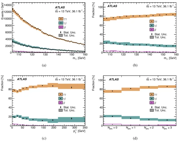
and relative fractions of the γγ , γ j and j j backgrounds are shown in Figure 3 as a function of m

for

the selected events. The fractions of these background sources in the inclusive diphoton sample are

(78 . 7

¹ ₅

⁸ ₂ )%, (18 . 6

⁴ 1

² 6 )% and (2 . 6

⁰ 0.4

⁵ )%, respectively. The uncertainties in the measured background

[GeV]

γ

mγ

110 120 130 140 150 160

Events / GeV

0 2000 4000 6000 8000 10000 12000

14000 ATLAS

= 13 TeV, 36.1 fb-1

s γ γ

j γ jj Stat. Unc.

Tot. Unc.

(a)

[GeV]

γ

mγ

110 120 130 140 150 160

Fraction [%]

0 20 40 60 80

100 ATLAS s = 13 TeV, 36.1 fb^-1

γ γ

j γ jj Stat. Unc.

Tot. Unc.

(b)

[GeV]

γ γ

pT

0 50 100 150 200 250 300 350

Fraction [%]

0 20 40 60 80

100 ATLAS s = 13 TeV, 36.1 fb^-1

γ γ

j γ jj Stat. Unc.

Tot. Unc.

(c)

jets = 0

N Njets = 1 Njets = 2 N_jets≥ 3

Fraction [%]

0 20 40 60 80

100 ATLAS s = 13 TeV, 36.1 fb^-1

γ γ

j γ jj Stat. Unc.

Tot. Unc.

(d)

Figure 3: The data-driven determination of (a) event yields and (b) event fractions for γγ, γ j and j j events as a function of m

after the final selection outlined in Section 5. The event fractions for two differential observables, (c) p

T

and (d) N

defined for jets with a p

> 30 GeV are shown as well. The shaded regions show the total uncertainty of the measured yield and fraction, and the error bars show the statistical uncertainties.

fractions are systematically dominated. These results are comparable to previous results at

√ s = 7 and 8 TeV [9, 76]. In addition the purity is shown as a function of the p _T of the diphoton system, and the number of reconstructed jets with p _T > 30 GeV.

The functional form used to model the background m

distribution in the fit to the data is chosen, in each region, to ensure a small bias in the extracted signal yield relative to its experimental precision, following the procedure described in Ref. [3]. The potential bias ( spurious signal ) is estimated as the maximum of the absolute value of the fitted signal yield, using a signal model with mass between 121 and 129 GeV, in fits to the background control regions described before.

The spurious signal is required, at 95% confidence level (CL), to be less than 10% of the expected SM

signal yield or less than 20% of the expected statistical uncertainty in the SM signal yield. In the case

when two or more functions satisfy those requirements, the background model with the least number

polynomial is tested against an exponential of a third-order polynomial) to check, using only events in the diphoton invariant mass sidebands ( i.e. excluding the range 121 GeV < m

< 129 GeV), if the data favors a more complex model. A test statistic is built from the χ ² values and number of degrees of freedom of two binned fits to the data with the two background models. The expected distribution of the test statistic is built from pseudo-data assuming that the function with fewer degrees of freedom is the true underlying model. The value of the test statistic obtained in the data is compared to such distribution, and the simpler model is rejected in favor of the more complex one if the p -value of such comparison is lower than 5%. The background distribution of all regions is found to be well modeled by at least one of the following functions: an exponential of a first- or second-order polynomial, a power law, or a third-order Bernstein polynomial.

6.3 Statistical model

The data are interpreted following the statistical procedure summarized in Ref. [92] and described in detail in Ref. [93]. An extended likelihood function is built from the number of observed events and invariant diphoton mass values of the observed events using the analytic functions describing the distributions of m

in the range 105–160 GeV for the signal and the background.

The likelihood for a given reconstructed category, fiducial region, or differential bin i of the integrated or differential cross-section measurement is a marked Poisson probability distribution,

L

= Pois (n

|N

(θ)) ·

ni

Ö

j=

1

f

(m

, θ) · G(θ),

where n

( N

) is the observed (expected) number of selected candidates, f

(m

) is the value of the probability density function (pdf) of the invariant mass distribution evaluated for each candidate j , θ are nuisance parameters and G(θ) is a set of unit Gaussian constraints on a subset of the nuisance parameters, as described in the following. The likelihood for the measurements of the total Higgs boson production-mode cross sections and signal strengths is given by the product of the likelihood functions of each event reconstruction category. For the fiducial integrated and differential cross- section measurements the likelihood of all bins i in a spectrum is taken.

The number of expected candidates is the sum of the signal and background yields, denoted by N

^sig and N

^bkg , and the fitted spurious signal yield, N

^spur · θ

^spur ,

N

= N

^sig + N

^bkg + N

^spur · θ ^spur

.

In more detail, the invariant mass distribution for each category has signal and background compon- ents,

f

(m

) = h

(N

^sig + N

^spur · θ ^spur

) · f

^sig (m

, θ

^sig ) + N

^bkg · f

^bkg (m

, θ

^bkg ) i /N

,

where θ

^sig and θ

^bkg are nuisance parameters associated with systematic uncertainties affecting the

resolutions and positions (Section 7.1) of the invariant mass distributions of the signal f

^sig (further

detailed in Section 6.1) or the shape of the background f

^bkg (as explained in Section 6.2), respectively.