Interpretations of the combined measurement of Higgs boson production and decay

ATLAS-CONF-2020-053 29October2020

ATLAS CONF Note

ATLAS-CONF-2020-053

28th October 2020

Interpretations of the combined measurement of Higgs boson production and decay

The ATLAS Collaboration

First combined measurements of the Higgs boson production and decay using up to 139 fb

of proton–proton collision data at

√s =

13 TeV recorded by the ATLAS experiment have recently been performed. This note presents two interpretations of these combined Higgs boson measurements. Measurements targeting Simplified Template Cross Sections in different decay channels are reparameterized in terms of the impact of Standard Model Effective Field Theory (SMEFT) operators and constraints are reported on the corresponding Wilson coefficients.

Measurements are furthermore interpreted in several MSSM benchmark scenarios, resulting in constraints on the MSSM parameters

, tan

that are complementary to those obtained from direct searches for additional Higgs bosons. For all interpretations, no significant deviations from the Standard Model are observed.

© 2020 CERN for the benefit of the ATLAS Collaboration.

Reproduction of this article or parts of it is allowed as specified in the CC-BY-4.0 license.

1 Introduction

Following the discovery of the Higgs boson (

) [1–6] by the ATLAS [7] and CMS [8] experiments, its properties have been probed in proton–proton (

) collision data produced by the Large Hadron Collider (LHC) at CERN. The ATLAS collaboration recently presented first results on the combination of Higgs boson production and decay rate measurements with up to 139 fb

of 13 TeV

collision data [9], collected during LHC Run 2 in the years 2015 through 2018.

Two interpretations of these measurements are presented here, based on an Effective Field Theory (EFT) framework of the Standard Model (SM), as well as a minimal supersymmetric extension of the Standard Model (MSSM).

Effective field theories provide a model-independent approach, systematically improvable with higher-order perturbative calculations, to parametrise the effects of candidate theories beyond the Standard Model (BSM) that reduce to the Standard Model at low energies. In SM Effective Field Theory (SMEFT), the effects of BSM dynamics at energy scales

that are large in comparison to the Higgs vacuum-expectation-value

(

) can be parametrised at low energies,

, in terms of higher-dimensional operators built up from the Standard Model fields and respecting its symmetries. Measurements of (fiducial) cross-sections allow constraining of the coefficients associated to each SMEFT operator, and hence put constraints on new physics at some fixed scale

, for which

1 TeV is used throughout this note. The methodology employed here is quite similar to the one used by the individual Higgs analyses, especially

4

(

=

or

) [10] and

¯ (

,

or

) [11, 12]. A similar combined measurement has previously been performed on a subset of the data [13], but the measurement technique has been significantly developed in Ref. [14]. Its application to the combined measurements of the

¯ (

),

4

and

channels comes with specific challenges, linked to the search of the set of operators that can be effectively probed in the combination, which can be different from the union of operators probed by each of the individual analyses, due to different correlations between production and decay of these channels.

Conversely, in the MSSM approach a combination of Higgs boson measurements in various decay channels is used, including besides

¯ (VH) [11],

4

[10] and

[15], vector-boson-fusion production of

¯ (VBF) [16] and

¯

[17], as well as

[18],

[19],

multilepton

¯ [20], and

[21]. These measurements are interpreted in a model- dependent way, assuming that the observed Higgs boson is the light CP-even Higgs boson of the minimal supersymmetric extension of the Standard Model. In the past years, measurements were interpreted [22]

in the hMSSM model [23], for various values of the mass of the neutral CP-odd boson

), and the ratio of the vacuum expectation values of the Higgs doublets (tan

). The use of this model as a benchmark MSSM scenario to study constraints in the

, tan

-plane suffers from limitations in regions with small

, or large tan

, or both low

and low tan

. Here, six more recent benchmark MSSM scenarios [24, 25] are tested, including two that were especially designed for the low tan

(<10) regime.

The note is structured as follows: Section 2 gives an overview of the combined Higgs couplings analysis

that is used as a baseline to derive the results presented. Section 3 describes the general approach of

deriving limits on Wilson coefficients, while Section 4 details the specific choices of Wilson coefficients

and their combinations probed in this analysis as well as the corresponding results. Similarly, Section 5

describes the approach taken to interpret the Higgs coupling measurements in the context of the MSSM,

while Section 6 presents the resulting limits in the

, tan

-plane. Finally, Section 7 presents the

conclusions.

2 Combined measurement of Higgs boson production and decay

The results of this note are based on

collision data collected by the ATLAS experiment1 [26–28] in the years from 2015 to 2018, with the LHC operating at a center-of-mass energy of 13 TeV. The decay channels, targeted production modes and integrated luminosities of the datasets used in each analysis are summarized in Table 1. The uncertainty on the combined 2015–2018 integrated luminosity is 1.7% [29], obtained using the LUCID-2 detector [30] for the primary luminosity measurements.

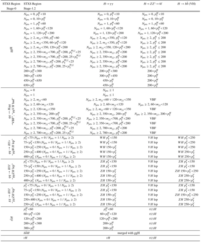
Table 1: The decay channels, targeted production modes and integrated luminosity (L) used for each input analysis of the combination. The references for the input analyses and information about which measurements they enter are also provided. The definition of the STXS stage of the signal yield parametrization is detailed in Section2.2.

Analysis Integrated Reference STXS Used in Used in

lumi (fb

) stage MSSM EFT

H→γγ

(all production modes) 139 [15] 1.2

H→Z Z^∗→

4

(all production modes) 139 [10] 1.2

H→bb

¯ (

) 139 [11] 1.2

H→W W^∗

(ggH, VBF) 36.1 [18] 1.0

-

H→ττ

(ggH, VBF) 36.1 [19] 1.0

-

H→bb

¯ (VBF) 24.5 – 30.6 [16] 0

-

H→bb

¯ (

) 36.1 [17] 0

-

H→

multilepton (

) 36.1 [20] 0

-

H→ µµ

(all production modes) 139 [21] 0

-

2.1 Simulation of the Standard Model signal

For each Higgs boson decay mode, the used branching fraction corresponds to theoretical calculations at the highest available order [31].

All analyses except

¯ (VBF) use a consistent set of Higgs boson signal samples which is described in the following paragraphs. The samples used for

¯ (VBF) are described separately at the end of this section.

Higgs boson production via gluon-gluon fusion (ggH) is simulated using the Powheg Box [32–35]

NNLOPS implementation [36, 37]. The event generator uses HNNLO [38] to reweight the inclusive Higgs boson rapidity distribution produced by the next-to-leading order (NLO) generation of

parton, with the scale of each parton emission determined using the MiNLO procedure [39]. The PDF4LHC15 parton distribution functions (PDFs) are used for the central prediction and uncertainty. The sample is normalized such that it reproduces the total cross section predicted by a next-to-next-to-next-to-leading- order (N

LO) QCD calculation with NLO electroweak corrections applied [31, 40–43]. The NNLOPS

1ATLAS uses a right-handed coordinate system with its origin at the nominal interaction point (IP) in the center of the detector and thez-axis along the beam pipe. Thex-axis points from the IP to the center of the LHC ring, and they-axis points upwards.

Cylindrical coordinates(r,φ)are used in the transverse plane,φbeing the azimuthal angle around thez-axis. The pseudorapidity is defined in terms of the polar angleθasη=−ln tan(θ/2). Angular distance is measured in units of∆R≡

q(∆η)²+(∆φ)².

generator reproduces the Higgs boson

distribution predicted by the NNLO plus next-to-next-to-leading logarithm (NNLL) calculation of Hres2.3 [44], which includes the effects of top- and bottom-quark masses and uses dynamical renormalization and factorization scales.

The VBF and

production processes are simulated at NLO accuracy in QCD using the Powheg Box [45]

generator with the PDF4LHC15 set of PDFs, where the simulation of

relies on improved NLO calculations [46]. The VBF sample is normalized to an approximate-NNLO QCD cross section with NLO electroweak corrections applied [31, 47–49]. The

samples are normalized to cross sections calculated at NNLO in QCD with NLO electroweak corrections [50, 51] and additional NLO QCD corrections [52]

for the

subprocess [31].

Higgs boson production in association with a top–antitop pair is simulated at NLO accuracy in QCD using the Powheg Box generator with the PDF4LHC15 set of PDFs for the

and

4

decay processes. For other Higgs boson decays, the MadGraph5_aMC@NLO [53] generator is used with the NNPDF3.0 set of PDFs. In both cases the sample is normalized to a calculation with NLO QCD and electroweak corrections [31, 54–57].

In addition to the primary Higgs boson processes, separate samples are used to model lower-rate processes.

For the 36 fb

analyses, Higgs boson production in association with a bottom–antibottom pair (

¯ ) is simulated using MadGraph5_aMC@NLO [58] with NNPDF2.3LO PDFs and is normalized to a cross section calculated to NNLO in QCD [31, 59–61]. The sample includes the effect of interference with the ggH production mechanism. Higgs boson production in association with a single top quark and a

boson (

) is produced at LO accuracy using MadGraph5_aMC@NLO. Finally, Higgs boson production in association with a single top quark in the t-channel (

) is generated at LO accuracy using MadGraph5_aMC@NLO with CT10 [62] PDF sets. The

samples are normalized to NLO QCD calculations [31, 63]. For the 139 fb

analyses, the PDF used for the

¯ sample is CT10, and the single top associated samples are produced at NLO accuracy in QCD using the NNPDF3.0NLO PDF set.

In the all-hadronic channel of the

¯ (VBF) analysis, the Powheg Box generator with the CT10 [62]

set of PDFs is used to simulate the ggH and VBF production processes, and interfaced with Pythia8 for parton shower. In the photon channel of the

¯ (VBF) analysis, VBF and ggH production in association with a photon is simulated using the MadGraph5_aMC@NLO generator with the PDF4LHC15 set of PDFs, and also using the Pythia8 generator for the parton shower. For both channels, contributions from

and

production are generated with Pythia8 generator with the NNPDF3.0 set of PDFs, and with MadGraph5_aMC@NLO showered with Herwig++ and using the NLO CT10 PDF, respectively.

All parton-level events are input to Pythia8 [64] to model the Higgs boson decay, parton showering, hadronization, and multiple parton interactions (MPI). The generators are interfaced to Pythia8, using the AZNLO and A14 parameter sets [65].

Particle-level events were passed through a Geant 4 [66] simulation of the ATLAS detector [67] and

reconstructed using the same analysis software as used for the data. Event pileup is included in the

simulation by overlaying inelastic

collisions, such that the average number of interactions per bunch

crossing reproduces that observed in the data. The inelastic

collisions were simulated with Pythia8 using

the MSTW2008lo [68] set of PDFs with the A2 [69] set of tuned parameters or using the NNPDF2.3LO

set of PDFs with the A3 [70] set of tuned parameters.

2.2 Signal yield parametrization

In all analyses listed in Table 1, the estimated contributions to the Higgs boson signal yield are separately parametrized for every contributing permutation of Higgs boson production/decay mode, i.e. the likelihood for each analysis region

is modeled as

L(N_k|µ^i,X

,

Poisson

N_k|s_k(µ^i,X

,

(1)

,

i,X

µ^i,X × L ×(σ×B)^i,X

SM,MC(θ)×^i,X_k (θ)

, (2)

where

is the observed event count,

is the expected signal count,

is the integrated luminosity,

is a scale parameter for the SM Higgs boson signal

SM,MC

used in the MC simulation with the indices

and

enumerating the considered production and decay modes. Furthermore,

represents the corresponding acceptances times efficiency,

represents the expected event count from background processes, and

represents the ensemble of nuisance parameters that describe the systematic uncertainties that originate from theoretical and experimental sources. Unlike the cross-section results presented in Ref. [9], which only account for signal theory uncertainties in migration effects that occur at the reconstruction level through the term

for the effect of theory uncertainties on the inclusive signal cross-section via the term

SM,MC(θ)

. For the analysis presented here, the scale factor

is factorized as

µ^i,X = σⁱ×B^H→X (σ×B)^i,X

SM,MC

, (3)

where

and

represent Higgs boson production cross sections and branching fractions respectively.

The Higgs boson production cross sections

are parameterized at a minimum granularity of inclusive production rates, labeled by LO process (

=ggH, VBF, . . . ). A more fine-grained definition of Higgs boson production cross sections additionally partitioned in particle-level kinematic regions, e.g. in bins of

, allow the ensemble of parameters

to describe deviations in differential distributions, with the level of detail controlled by the number of particle-level regions

that are defined. Conversely, the precision with which this more fine-grained ensemble of parameters

can be measured depends on the design of the analysis as well as the amount of available data. Analysis regions

, defined at the reconstruction level, are typically chosen to match the particle-level regions

as closely as possible, in order to reduce the extrapolation uncertainty. As reconstruction-level selections do generally not correspond exactly to particle level regions, multiple particle-level regions

will contribute to the signal yield

of Eq. (2).

For an interpretation of the measured Higgs boson data in a particular physics model (SMEFT, MSSM)

with parameters

, the original model parameters

and

are replaced with functional expressions

that parameterize the predictions of the model,

and

, so that the likelihood of Eq. (1) is

directly expressed in the parameters

, and constraints on these parameters can be directly inferred from the

modified likelihood expression. While the original parameters

no longer appear in the reparameterized

expression, the granularity of the definition of the regions that defined

will continue to be a relevant

factor in the achievable level of detail in the parameterization in

.

For the analyses presented here, regions in Higgs boson production phase space known as simplified template cross sections [31, 71–73] (STXS) are used. STXS regions are defined in terms of the kinematics of the Higgs boson and, when they are present, of associated jets and

and

bosons, independently of the Higgs boson decay process. Partitions are chosen according to three criteria: sensitivity to deviations from the SM expectation, avoidance of large theory uncertainties in the corresponding SM predictions, and approximately matching experimental selections so as to minimize model-dependent extrapolations with respect to e.g. the acceptance factor of the STXS bins. All STXS regions are defined for a Higgs boson rapidity

satisfying

2.5, corresponding approximately to the region of experimental sensitivity.

Jets are reconstructed from all stable particles with an average lifetime greater than 10 ps, excluding the decay products of the Higgs boson and leptons from

and

boson decays, using the anti-

algorithm with a jet radius parameter

0.4, and must have a transverse momentum

30 GeV. Higgs boson production is first classified according to the nature of the initial state and the associated particles, the latter including the decay products of the

and

bosons if they are present. These classes are:

and

processes;

processes, with contributions from both VBF production and quark-initiated

production with a hadronic decay of the gauge boson;

production with a leptonic decay of the vector boson (

(lep)

), including

production; and finally the ggH process. The last process is considered together with

,

¯ production, as a single

process. The

¯ production mode is modeled as a 1% [31] increase of the

yield in each STXS cross section, since the acceptances for both processes are similar for all input analyses [31]. Theory uncertainties for the

,

, and

processes are defined as in Ref. [10, 15], while those of the

(lep)

process follow the scheme described in Ref. [74].

For each production mode, multiple levels of progressively more detailed partitioning are defined with STXS stages [31]. The most detailed Stage 1.2 splitting of the STXS framework is implemented by the 139 fb

measurements of

¯ (VH),

4

and

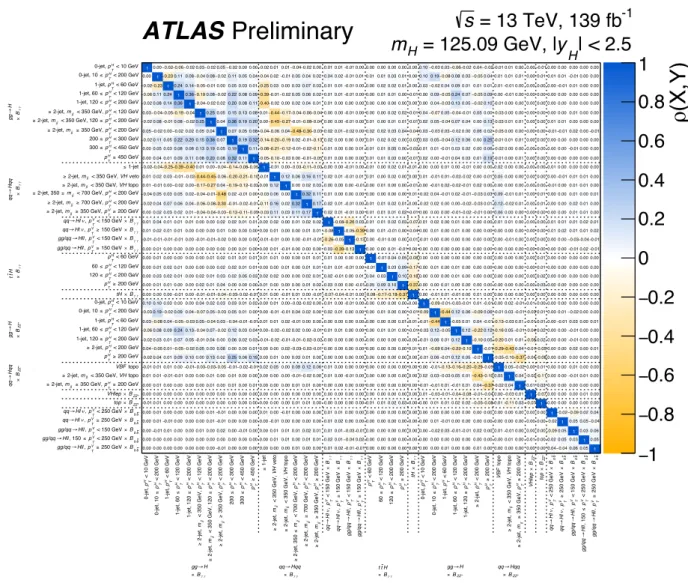
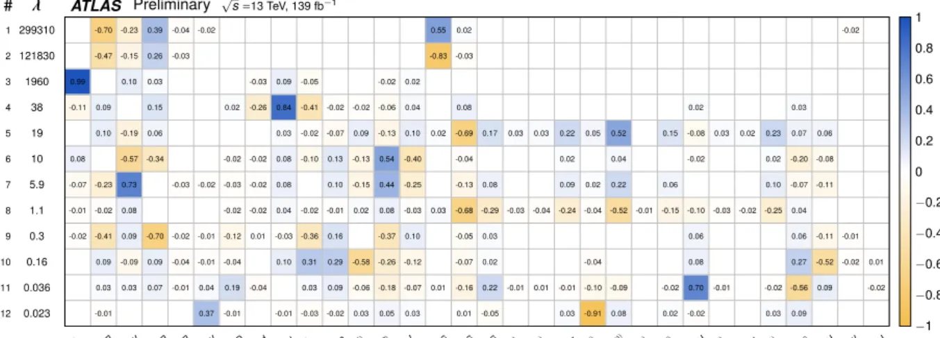
presented in this note, which allows for their use in the EFT interpretation analysis. However, as the individual analyses provide only limited sensitivity to some of the Stage 1.2 categories, some of these categories are merged for the combined EFT analysis. The mapping of the merged EFT regions to the STXS Stage 1.2 regions is detailed in Table 2, and the corresponding measured signal strengths and their correlations are shown in Fig. 1 and Fig. 2 respectively. For the measurement bins defined by merging several bins of the STXS Stage-1.2 framework, the efficiency and acceptance factors

are determined using SM predictions for the relative fraction of each Stage-1.2 bin. SM uncertainties in these fractions are taken into account.

For the MSSM interpretation only inclusive cross section predictions are available, hence STXS Stage 1.2

regions do not represent a useful level of detail for this interpretation. Therefore, for the MSSM analysis all

STXS-1.2 cross sections are merged into the six Stage-0 cross sections (as defined in the first column of

Table 2.) Therefore, the MSSM interpretation can include six additional Higgs boson analyses that are only

available in more coarse-grained STXS levels (Level 0 and 1.0), as shown in Table 1.

4

− − 2 0 2 4 6

μ

Total Stat.

Syst. SM

Preliminary ATLAS

= 13 TeV, 139 fb-1

sH = 125.09 GeV, |y_H| < 2.5 m_SM = 91%

p

b

Bb

Hll× gg/qq→

b

Bb

ν× Hl qq→

BZZ*

top× BZZ*

VHlep× BZZ*

Hqq× qq→

BZZ*

H× gg→

γ

Bγ

tH×

γ

Bγ

H× tt

γ

Bγ

Hll× gg/qq→

γ

Bγ

× Hlν qq→

γ

Bγ

Hqq× qq→

γ

Bγ

H× gg→

Total Stat. Syst.

< 10 GeV

HT

p

0-jet, 0.75 ₋⁺_0.30^0.32 (±0.25, ₋⁺_0.17^0.21)

< 200 GeV

HT

p

0-jet, 10 ≤ 1.22 ₋⁺_0.22^0.24 (±0.15, ₋⁺_0.15^0.19)

< 60 GeV

H

pT

1-jet, 0.92 ₋⁺_0.44^0.51 (±0.39, ₋⁺_0.21^0.33)

< 120 GeV

H

pT

1-jet, 60 ≤ 1.25 ₋⁺_0.42^0.53 (₋⁺_0.36^0.35, ₋⁺_0.23^0.39)

< 200 GeV

HT

p

1-jet, 120 ≤ 0.72 ₋⁺_0.48^0.61 (₋⁺_0.46^0.47, ₋⁺_0.13^0.39)

< 120 GeV

H

pT

< 350 GeV, mjj

2-jet,

≥ 0.24 ₋⁺_0.50^0.54 (₋⁺_0.46^0.47, ₋⁺_0.20^0.28)

< 200 GeV

H

pT

< 350 GeV, 120 ≤ mjj

2-jet,

≥ 0.60 ₋⁺_0.45^0.56 (₋⁺_0.40^0.41, ₋⁺_0.20^0.39)

< 200 GeV

HT

p 350 GeV,

jj≥ m 2-jet,

≥ 2.02 ₋⁺_0.93^1.18 (₋⁺_0.77^0.78, ₋⁺_0.52^0.88)

< 300 GeV

HT

p

200 ≤ 0.97 ₋⁺_0.39^0.53 (₋⁺_0.33^0.34, ₋⁺_0.21^0.41)

< 450 GeV

HT

p

300 ≤ 0.21 ₋⁺_0.47^0.58 (₋⁺_0.43^0.49, ₋⁺_0.19^0.32)

450 GeV

H≥

pT 1.51 ₋⁺_1.06^1.76 (₋⁺_0.97^1.21, ₋⁺_0.44^1.29)

1-jet

≤ 1.48 ₋⁺_1.07^1.20 (₋⁺_1.01^1.14, ₋⁺_0.33^0.36)

veto VH < 350 GeV, mjj

2-jet,

≥ 3.03 ₋⁺_1.73^1.87 (₋⁺_1.63^1.71, ₋⁺_0.58^0.77)

topo VH < 350 GeV, mjj

2-jet,

≥ 0.67 ₋⁺_0.81^0.93 (₋⁺_0.77^0.88, ₋⁺_0.25^0.28)

< 200 GeV

H

pT

< 700 GeV, mjj

2-jet, 350 ≤

≥ 0.88 ₋⁺_0.67^0.81 (₋⁺_0.60^0.66, ₋⁺_0.29^0.46)

< 200 GeV

HT

p 700 GeV,

jj≥ m 2-jet,

≥ 1.11 ₋⁺_0.33^0.39 (₋⁺_0.27^0.28, ₋⁺_0.20^0.27)

200 GeV

H≥ pT

350 GeV,

jj≥ m 2-jet,

≥ 1.34 ₋⁺_0.41^0.47 (₋⁺_0.37^0.42, ₋⁺_0.17^0.21)

< 150 GeV

V

pT 2.41 ₋⁺_0.67^0.74 (₋⁺_0.66^0.72, ₋⁺_0.12^0.18)

150 GeV

V≥

pT 2.65 ₋⁺_1.00^1.18 (₋⁺_0.98^1.15, ₋⁺_0.19^0.27)

< 150 GeV

VT

p -1.09 ₋⁺_0.02^0.97 (₋⁺_0.02^0.96, ₋⁺_0.00^0.15)

150 GeV

V≥

pT -0.10 ₋⁺_0.95^1.14 (₋⁺_0.91^1.11, ₋⁺_0.25^0.26)

< 60 GeV

H

pT 0.74 ₋⁺_0.68^0.83 (₋⁺_0.68^0.79, ₋⁺_0.09^0.24)

< 120 GeV

HT

p

60 ≤ 0.71 ₋⁺_0.45^0.55 (₋⁺_0.45^0.53, ₋⁺_0.06^0.15)

< 200 GeV

HT

p

120 ≤ 1.05 ₋⁺_0.54^0.65 (₋⁺_0.52^0.60, ₋⁺_0.13^0.25)

200 GeV

H≥

pT 0.95 ₋⁺_0.47^0.57 (₋⁺_0.46^0.52, ₋⁺_0.10^0.23)

0.68)

− 0.79 , + 2.30

− 3.15 (+ 2.40

− 3.25 0.77 +

< 10 GeV

HT

p

0-jet, 0.95 ₋⁺_0.31^0.38 (₋⁺_0.28^0.31, ₋⁺_0.14^0.21)

< 200 GeV

HT

p

0-jet, 10 ≤ 1.14 ₋⁺_0.20^0.23 (₋⁺_0.16^0.17, ₋⁺_0.12^0.15)

< 60 GeV

H

pT

1-jet, 0.23 ₋⁺_0.42^0.44 (₋⁺_0.35^0.39, ₋⁺_0.22^0.20)

< 120 GeV

HT

p

1-jet, 60 ≤ 1.43 ₋⁺_0.42^0.52 (₋⁺_0.37^0.41, ₋⁺_0.19^0.31)

< 200 GeV

HT

p

1-jet, 120 ≤ 0.45 ₋⁺_0.57^0.83 (₋⁺_0.57^0.78, ₋⁺_0.08^0.27)

< 200 GeV

H

pT

2-jet,

≥ 0.27 ₋⁺_0.51^0.56 (₋⁺_0.47^0.50, ₋⁺_0.19^0.23)

200 GeV

H≥

pT 2.27 ₋⁺_1.04^1.55 (₋⁺_0.97^1.23, ₋⁺_0.38^0.95)

topo

VBF 1.43 ₋⁺_0.49^0.61 (₋⁺_0.48^0.58, ₋⁺_0.09^0.17)

topo VH < 350 GeV, mjj

2-jet,

≥ 1.59 ₋⁺_2.14^2.70 (₋⁺_2.10^2.64, ₋⁺_0.41^0.59)

200 GeV

H≥ pT

350 GeV,

jj≥ m 2-jet,

≥ 0.05 ₋⁺_1.17^1.92 (₋⁺_1.15^1.91, ₋⁺_0.22^0.18)

0.05)

−0.16 , + 1.06

−1.68 (+ 1.06

−1.68 1.32 +

0.18)

−0.40 , + 1.09

−1.67 (+ 1.10

−1.72 1.65 +

< 250 GeV

VT

p 0.78 ₋⁺_0.48^0.49 (₋⁺_0.30^0.31, ₋⁺_0.38^0.39)

250 GeV

V≥

pT 1.01 ₋⁺_0.30^0.32 (₋⁺_0.25^0.27, ₋⁺_0.16^0.18)

< 150 GeV

VT

p 0.84 ₋⁺_0.70^0.74 (₋⁺_0.46^0.47, ₋⁺_0.53^0.57)

< 250 GeV

VT

p

150 ≤ 1.10 ₋⁺_0.33^0.35 (±0.26, ₋⁺_0.20^0.23)

250 GeV

V≥

pT 1.09 ₋⁺_0.31^0.34 (₋⁺_0.28^0.29, ₋⁺_0.14^0.17)

_

-

-

Figure 1: Measured signal strength for each STXS category entering the EFT analysis. The corresponding categories are defined in Table2. Input data taken from Ref. [9]. The probability to obtain the observed data under the SM hypothesis (p ) is 91%.