Constraints on New Phenomena via Higgs Boson Coupling Measurements with the ATLAS Detector

ATLAS-CONF-2014-010 22/04/2014

ATLAS NOTE

ATLAS-CONF-2014-010

March 24, 2014 Revision: April 22, 2014

Constraints on New Phenomena via Higgs Boson Coupling Measurements with the ATLAS Detector

The ATLAS Collaboration

Abstract

The ATLAS experiment at the LHC has determined the couplings of the Higgs boson to other particles, as well as its mass, using the combination of measurements from multiple production and decay channels with up to 4.8 fb

of

collision data at

s=

7 TeV and 20.3 fb

at

s=

8 TeV. In this study, the mass dependence of the couplings is probed and the coupling measurements are interpreted in di

erent extensions of the Standard Model. An indirect search is performed for a composite Higgs boson, an additional electroweak singlet, an additional electroweak doublet (two-Higgs-doublet model), a simplified Minimal Super- symmetric Standard Model, and a Higgs portal to dark matter. The measured production and decay rates of the observed Higgs boson in the

4`,

¯ channels, the measured mass in the

and

4` decay modes, and the measured upper limit on the rate of the

process are used to constrain parameters of these models.

Figure 7 has been updated to correct an error in the calculation of the ATLAS upper limits on the WIMP-nucleon scattering cross sectionσ_χ−N in the Higgs portal model; the corrected limits are 1.59 times higher. The limits on the Higgs boson invisible branching ratio are not affected.

c

Copyright 2014 CERN for the benefit of the ATLAS Collaboration.

Reproduction of this article or parts of it is allowed as specified in the CC-BY-3.0 license.

1 INTRODUCTION

1

1 Introduction

The ATLAS and CMS Collaborations at the Large Hadron Collider (LHC) announced the discovery of a Higgs-like boson in the summer of 2012 [1, 2]. Since then, both collaborations have measured the mass of the particle to be approximately 125.5 GeV [3, 4]. Studies of its spin and parity have found it to be compatible with a J

0

state [5–7]. Combined coupling fits of the measured production and decay rates within the framework of the Standard Model (SM) have found no significant deviation from the SM expectations [3, 4]. These results strongly suggest that the newly-discovered particle is indeed a Higgs boson and that a non-zero vacuum expectation value of a Higgs doublet is responsible for electroweak (EW) symmetry breaking [8–10]. A crucial question is whether there is only one Higgs doublet as postulated by the SM, or whether the Higgs sector is extended, leading to more than one Higgs boson of which one has SM-like properties, as predicted in many beyond-Standard-Model (BSM) theories. The

“hierarchy problem” regarding the naturalness of the Higgs boson mass, the nature of dark matter, and other open questions that the SM is not able to answer also motivate the possible existence of additional new particles and interactions.

This note reports an indirect search for various BSM models that could address these issues, per- formed using the Higgs boson production and decay rate measurements and a direct search for invisible decays of the Higgs boson. The statistical methods used are described in Sec. 2. The mass dependence of the couplings is probed in Sec. 3. The rate measurements are used to derive limits on five representative classes of models: Higgs boson compositeness in Sec. 4, an additional electroweak singlet in Sec. 5, an additional electroweak doublet (two-Higgs-doublet model) in Sec. 6, a simplified Minimal Supersym- metric Standard Model (MSSM) in Sec. 7, and a Higgs portal to dark matter in Sec. 8. These models modify the couplings of the Higgs boson to fermions and vector bosons by functions of the parameters of the BSM theory. In all cases, it is assumed that the modifications of the couplings do not change the Higgs boson decay kinematics appreciably, so that the expected rate of any given process can be obtained through a simple rescaling of the SM couplings.

A simultaneous fit of the measured rates in multiple production and decay modes is used to constrain the BSM model parameters. The experimental inputs are measurements in the h

γγ, h

ZZ

4`, h

WW

`ν`ν [3], h

ττ [11], and h

b b ¯ [12] channels, based on up to 4.8 fb

of pp collision data at

s

7 TeV and 20.3 fb

at

s

8 TeV.

The combination of measurements in these channels and the derivation of the Higgs boson couplings are described in Ref. [13]. Measurements of the couplings and invisible branching ratio in various parametrizations, along with the BSM models they are used to probe, are given in Table 1. The measured upper limit on the rate of the process Zh

``

E

[14] is also used, in addition to the channels above, to constrain the branching ratio of the Higgs boson to invisible final states. Direct searches for additional Higgs bosons and other new phenomena provide additional constraints on some of these models, but are not considered in the current analysis.

2 Statistical Analysis

The statistical treatment of the data is described in Refs. [15–19]. Confidence intervals are based on the profile likelihood ratio [20]

(α) test statistic:

t

(1)

1The observed light, CP-even Higgs boson with a mass of 125.5 GeV is denoted ashthroughout the note.

2 STATISTICAL ANALYSIS

2

Model Coupling

Parameter

Description Measurement

1 MCHM4,

EW singlet

µ_h Overall signal strength 1.30⁺_−0.17^0.18 κ= √

µ_h Universal coupling 1.14⁺_−0.08^0.09

2 MCHM5,

2HDM Type I

κV

Vector boson (W,Z)

coupling 1.15±0.08

κ_F Fermion (t,b,τ, . . . )

coupling 0.99⁺_−0.15^0.17

3 2HDM Type II, MSSM

λVu=κV/κu

Ratio of vector boson &

up-type fermion (t,c, . . . ) couplings

1.21⁺_−0.26^0.24

κuu =κ²_u/κh

Ratio of squared up-type fermion coupling & total width scale factor

0.86⁺_−0.21^0.41

λ_du=κ_d/κ_u

Ratio of down-type fermion (b,τ, . . . ) &

up-type fermion couplings

[−1.24,−0.81]∪[0.78,1.15]

4 2HDM Type III

λVq=κV/κq

Ratio of vector boson &

quark (t,b, . . . ) couplings 1.27⁺_−0.20^0.23 κ_qq =κ²_q/κ_h Ratio of squared quark

coupling & total width scale factor

0.82⁺_−0.19^0.23

λ_lq=κ_l/κ_q Ratio of lepton (τ,µ,e)

& quark couplings [−1.48,−0.99]∪[0.99,1.50]

5 Mass scaling parametrization

κZ Zboson coupling 0.95⁺_−0.19^0.24

κ_W Wboson coupling 0.68⁺_−0.14^0.30

κt tquark coupling [−0.80,−0.50]∪[0.61,0.80]

κb bquark coupling [−0.7,0.7]

κ_τ τlepton coupling [−1.15,−0.67]∪[0.67,1.14]

6

Higgs portal (without

Zh→``+E^miss_T )

κ_g Gluon effective coupling 1.00⁺_−0.16^0.23 κγ Photon effective coupling 1.17⁺_−0.13^0.16 BR_i Invisible branching ratio −0.16⁺_−0.30^0.29

7

Higgs portal (with

Zh→``+E^miss_T )

κ_g Gluon effective coupling –

κγ Photon effective coupling –

BR_i Invisible branching ratio −0.02±0.20

Table 1: Measurements of Higgs boson coupling scale factors in di

erent coupling parametrizations [13],

along with the BSM models or parametrizations they are used to probe. The production modes are

assumed to be the same as those in the SM in all cases. In models 1, 2, and 5, decay modes identical

to those in the SM are assumed. For models 3 and 4, the coupling parametrizations and measurements

listed do not require such an assumption, which is however made when deriving limits on the underlying

parameters of these BSM models. No assumption about the total width is made for models 6 and 7.

3 MASS SCALING OF COUPLINGS

3

where

Λ

(α)

L

,

ˆˆ

L( ˆ

ˆ . (2)

The single circumflex in the denominator of Eq. 2 denotes the unconditional maximum likelihood esti- mate of a parameter. The double circumflex in the numerator denotes the “profiled” value, namely the conditional maximum likelihood estimate for given fixed values of the parameters of interest

The likelihood in Eq. 2 depends on one or more parameters of interest

production strength µ normalized to the SM expectation (so that µ

1 corresponds to the SM Higgs boson hypothesis and µ

0 to the background-only hypothesis), the mass m

, coupling strengths

, as well as on nuisance parameters

built as a product of the likelihoods of all measured Higgs boson channels, where for each channel the likelihood is built using sums of signal and background probability density functions (PDFs) in the discriminating variables. These discriminants are chosen to be the γγ, 4`, and 2b-jet mass spectra for h

γγ, h

ZZ

4`, and h

b b, respectively; the transverse mass, ¯ m

, distribution for h

WW

`ν`ν; the distribution of a boosted decision tree response for h

ττ; and the missing transverse momentum, E

, distribution for the Zh

``

E

channel. The PDFs are derived from Monte Carlo (MC) simulation for the signal and from both data and simulation for the background.

Systematic uncertainties and their correlations [15] are modeled by introducing nuisance parameters

Confidence intervals are extracted by assuming t

follows an asymptotic χ

distribution with the corresponding number of degrees of freedom. For the composite Higgs boson, EW singlet, and Higgs portal models, a physical boundary imposes a lower bound on the model parameter under study. The maximum likelihood estimate and its uncertainty are first quoted ignoring the boundary, to provide the information corresponding directly to the measurements. The confidence intervals that are subsequently reported are based on the profile likelihood ratio where parameters are restricted to the allowed region of parameter space, as in the case of the ˜ t

test statistic described in Ref. [20]. This restriction of the like- lihood ratio to the allowed region of parameter space is similar to the Feldman-Cousins technique [21];

however, the confidence interval is defined by the standard χ

cutoff, which leads to some overcoverage near the boundaries. The Higgs boson couplings also have boundaries in the two-Higgs-doublet models and simplified MSSM, which are treated in a similar fashion.

3 Mass Scaling of Couplings

The observed rates in di

erent channels are used to determine the mass dependence of the Higgs boson couplings to other particles. The couplings are parametrized using scale factors denoted κ

, which are defined as the ratios between the couplings and their corresponding SM values for m

125.5 GeV. The measurements of the scale factors for the couplings of the Higgs boson to the Z boson, W boson, top quark, bottom quark, and τ lepton are given in Model 5 of Table 1.

The coupling scale factors to different species of fermions and vector bosons, respectively, are ex- pressed in terms of a mass scaling parameter and a “vacuum expectation value” parameter M [22]:

κ

v

M¹⁺

κ

v

,

(3)

where v

246 GeV is the vacuum expectation value in the SM, m

denotes the mass of each fermion

species (indexed i), and m

denotes each vector boson mass (indexed j). The mass-scaling dependence

of the couplings, and the vacuum expectation value, of the SM are recovered with parameter values

0

and M

v, which produce κ

κ

1.

4 MINIMAL COMPOSITE HIGGS MODEL

4 The production and decay rates are modified from their SM expectations accordingly. For example, assuming the narrow-width approximation [23, 24], the rate for the process gg

h

ZZ

4` relative to the SM prediction can be parametrized as [25]:

µ

. (4)

Here κ

is the scale factor for the loop-induced coupling to the gluon through the top and bottom quarks, where both the top and bottom couplings are scaled by κ

, and κ

is the coupling scale factor for the Z boson. The scale factor for the total width of the Higgs boson, κ

, is calculated as a squared e

ective coupling scale factor. It is defined as the sum of squared coupling scale factors for all decay modes, κ

, each weighted by the corresponding SM branching ratio:

κ

i

κ

BR

, (5)

where the summation is taken over all decay modes. The production and decay modes are assumed to be the same as those in the SM. Production or decays through loops are resolved in terms of the contributing particles in the loops, assuming the same mixture of contributions as in the SM. For example, the W boson provides the dominant contribution, followed by the top quark, to the h

γγ decay, such that the e

ective coupling scale factor κ

at m

125.5 GeV is given by:

κ

0.26κ

, (6) where the negative interference between the W and top loops, as well as the contributions from other particles in the loops, are accounted for.

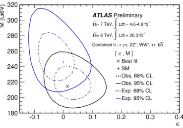
Combined fits to the measured rates are performed with the mass scaling factor and the vacuum expectation value parameter M as the two parameters of interest. Figure 1 shows the two-dimensional likelihood scan as a function of and M. The best-fit point is compatible with the expectation for the SM Higgs boson within approximately 1.5σ. The extracted value of is close to 0, indicating that the measured couplings to fermions and vector bosons are consistent with the linear and quadratic mass dependence, respectively, predicted in the SM. The best-fit value for M is less than v

246 GeV since the measured overall signal strength µ

is greater than 1.

4 Minimal Composite Higgs Model

Minimal Composite Higgs Models (MCHM) [26–28] represent another possible explanation for the scalar naturalness problem, wherein the Higgs boson is a composite, pseudo-Nambu-Goldstone bo- son rather than an elementary particle. In such cases, the Higgs boson couplings to vector bosons and fermions are modified with respect to their SM expectations as a function of the Higgs boson compos- iteness scale, f . It is assumed here that corrections due to new heavy resonances such as vector-like quarks [29] are sub-dominant.

In the MCHM4 model [26], the ratio of the predicted couplings to their SM expectations can be written in the particularly simple form:

κ

κ

κ

1

ξ, (7)

where ξ

v

/ f

is a scaling parameter such that the SM is recovered in the limit ξ

0, namely f

The combined signal strength, µ

, and equivalent coupling scale factor, κ

µ

, measured using the

combination of all considered channels are listed in Model 1 of Table 1. The experimental measurements

4 MINIMAL COMPOSITE HIGGS MODEL

5

-0.1 0 0.1 0.2 0.3 0.4∈

M [GeV]

180 200 220 240 260 280 300 320

, M ]

∈ [

Best fit SM Obs. 68% CL Obs. 95% CL Exp. 68% CL Exp. 95% CL Preliminary ATLAS

b τ, b τ , ZZ*, WW*, γ γ

→ Combined h

Ldt = 4.6-4.8 fb-1

∫

= 7 TeV, s

Ldt = 20.3 fb-1

∫

= 8 TeV, s

Figure 1: Two-dimensional likelihood scan of the mass scaling factor, , and the vacuum expectation value parameter, M. The likelihood contours where

2.3 and

6.0, corresponding approximately to 68% CL (1σ) and 95% CL (2σ) respectively, are shown for both the data and the prediction for a SM Higgs boson. The best fit to the data and the SM expectation are indicated as

and

respectively.

are interpreted in the MCHM4 scenario by rescaling the rates in di

erent production and decay modes as functions of the couplings κ

κ

κ

, assuming the same production and decay modes as in the SM.

The couplings are in turn expressed as functions of ξ using Eq. 7.

The MCHM4 model contains a physical boundary ξ

0, with the SM Higgs boson corresponding to ξ

0. Ignoring this boundary, the scaling parameter is measured to be ξ

1

µ

0.30

, while the expectation assuming the SM Higgs boson is 0.00

. The best-fit value observed for ξ is negative since µ

>1 is measured. The statistical and systematic uncertainties are of similar size. Accounting for the lower boundary produces an observed (expected) 95% CL upper limit of ξ < 0.12 (0.29), corresponding to a Higgs boson compositeness scale of f >710 GeV (460 GeV). The observed limit is stronger than expected since µ

>1 is measured.

Similarly, in the MCHM5 model [27, 28] the measured rates are expressed in terms of ξ by rewriting the couplings as:

κ

1

ξ κ

1−ξ

. (8)

The measurements of κ

and κ

are given in Model 2 of Table 1. As with the MCHM4 model, the MCHM5 model contains the physical boundary ξ

0, with the SM Higgs boson corresponding to ξ

0.

Ignoring this boundary, the composite Higgs boson scaling parameter is determined to be ξ

, while 0.00

is expected assuming the SM Higgs boson. As above, the best-fit value for ξ is negative since µ

>1 is measured. Accounting for the boundary produces an observed (expected) 95% CL upper limit of ξ < 0.15 (0.20), corresponding to a Higgs boson compositeness scale of f >640 GeV (550 GeV).

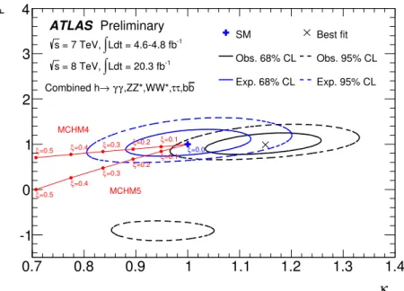
Figure 2 shows the two-dimensional likelihood for vector boson (κ

) and fermion (κ

) coupling measure-

ments in the (κ

, κ

) plane, overlaid with predictions as parametric functions of ξ for the MCHM4 and

MCHM5 models. A secondary minimum in the likelihood exists at κ

< 0 due primarily to the large

measured h

γγ rate [13].

5 ADDITIONAL ELECTROWEAK SINGLET

6

κV

0.7 0.8 0.9 1 1.1 1.2 1.3 1.4

Fκ

-1 0 1 2 3 4

SM Best fit

Obs. 68% CL Obs. 95% CL Exp. 68% CL Exp. 95% CL

ATLAS Preliminary

Ldt = 4.6-4.8 fb-1

∫

= 7 TeV, s

Ldt = 20.3 fb-1

∫

= 8 TeV, s

b τ,b τ ,ZZ*,WW*, γ

γ

→ Combined h

ξ=0.1 ξ=0.2 ξ=0.3 ξ=0.4

ξ=0.5 ξ=0.0

ξ=0.1 ξ=0.2 ξ=0.3 ξ=0.4 ξ=0.5

MCHM4

MCHM5

Figure 2: Two-dimensional likelihood contours in the (κ

, κ

) coupling plane, where

2 ln

2.3 and

−2 lnΛ =

6.0 correspond approximately to 68% CL (1σ) and 95% CL (2σ) respectively. The coupling predictions in the MCHM4 and MCHM5 models are shown as parametric functions of the Higgs boson compositeness parameter ξ

v

/ f

. The two-dimensional likelihood contours are shown for reference and should not be used to estimate the exclusion for the single parameter ξ.

5 Additional Electroweak Singlet

The simplest extension to the SM Higgs sector involves the addition of an EW singlet field [25, 30–35]

to the doublet Higgs field of the SM, providing a possible answer to the dark matter problem. Both fields acquire non-zero vacuum expectation values. Spontaneous symmetry breaking leads to mixing between the singlet state and the surviving state of the doublet field, resulting in two CP-even Higgs bosons, where h (H) denotes the lighter (heavier) of the pair. The two Higgs bosons, h and H, are assumed to be non-degenerate. They couple to fermions and vector bosons in a similar way as the SM Higgs boson, but each with a strength reduced by a common scale factor, denoted as κ for h and κ

for H. The constraint of unitarity implies that:

κ

κ

1. (9)

In this model, the lighter Higgs boson h is assumed to have identical production and decay modes to those of the SM Higgs boson, but with rates modified according to:

σ

κ

σ

κ

BR

BR

,

(10)

where σ denotes the production cross section,

denotes the total decay width, BR denotes the branching ratio, and i indexes the different decay modes.

For the heavier Higgs boson H, new decay modes such as H

hh are possible if they are kinemati-

cally accessible. In this case, the production and decay rates of the H boson are modified with respect to

6 TWO-HIGGS-DOUBLET MODEL

7 those of a SM Higgs boson with equal mass by the branching ratio of all new decay modes, BR

, as:

σ

κ

σ

κ

1

BR

BR

(1

BR

)

BR

.

(11)

Here σ

,

, and BR

denote the cross section, total width, and branching ratio for a given decay mode (indexed i) predicted for a SM Higgs boson with mass m

.

Consequently the overall signal strength, namely the ratio of production and decay rates in the mea- sured channels relative to the expectations for a SM Higgs boson with corresponding mass, is given by:

µ

σ

BR

(σ

BR

)

κ

µ

σ

BR

(σ

BR

)

κ

1

BR

(12)

for h and H respectively, assuming the narrow-width approximation.

Combining Eqs. 9 and 12, the squared coupling of the heavy Higgs boson can be expressed in terms of the signal strength of the light Higgs boson as:

κ

1

µ

. (13)

The signal strength of the light Higgs boson, measured using the combination of all considered channels, is given in Model 1 of Table 1. The EW singlet model contains the physical boundary κ

0, with the SM corresponding to κ

0. Ignoring this boundary, the squared coupling of the heavy Higgs boson is measured to be κ

1

µ

, where the best-fit value is approximately 1.5σ below the physical boundary. The expectation is 0.00

.

Accounting for the lower boundary yields an observed (expected) 95% CL upper limit of κ

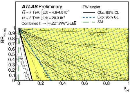
< 0.12 (0.29). From Eqs. 12, this corresponds to the maximum signal strength for contamination of a heavy Higgs boson into the light Higgs boson signal. Figure 3 shows the limits in the (µ

, BR

) plane of the heavy Higgs boson. Contours of the scale factor for the total width,

/

, and κ

, based on Eqs. 11 and 12, are also illustrated.

6 Two-Higgs-Doublet Model

Another simple extension of the SM Higgs sector is a class of models termed “Two-Higgs-Doublet Models” (2HDMs) [25, 36–38], in which the SM Higgs sector is extended by an additional doublet.

A concrete example of this model is realized in the Minimal Supersymmetric Standard Model since supersymmetry requires a second Higgs doublet, one coupling only to up-type quarks and the other only to down-type quarks and leptons.

2HDMs predict the existence of five Higgs bosons: two neutral CP-even bosons h and H, one neutral

CP-odd boson A, and two charged bosons H

. The most general 2HDMs predict CP-violating Higgs

boson couplings as well as tree-level flavor changing neutral currents. Since the latter are strongly

constrained by existing data, the models considered have additional requirements imposed, such as the

Glashow-Weinberg condition [39, 40], in order to evade existing experimental bounds.

6 TWO-HIGGS-DOUBLET MODEL

8

µH

=0.1² κ’

=0.2² κ’

=0.3² κ’

=0.42

κ’

=0.52

κ’

=0.62

κ’

2=0.7 κ’

2=0.8 κ’

2=0.9 κ’

2=1.0 κ’

=0.1

H,SMΓ

HΓ/

H,SM=0.5 /Γ

ΓH ΓH/Γ^H,SM=1.0

=5.0 ΓH,SM H/ Γ

H,SM=100 Γ

H/ Γ

ATLASPreliminary

Ldt = 4.6-4.8 fb-1

∫

= 7 TeV:

s

Ldt = 20.3 fb-1

∫

= 8 TeV:

s

b τ,b ,ZZ*,WW*,τ γ

γ Combined h →

EW singlet

Obs. 95% CL Exp. 95% CL SM

0 0.2 0.4 0.6 0.8 1

H,newBR

0 0.1 0.2 0.3 0.4 0.5 0.6 0.7 0.8 0.9 1

Figure 3: Observed and expected upper limits at 95% CL on the squared coupling, κ

, of a heavy Higgs boson arising through an additional EW singlet, shown in the (µ

, BR

) plane. The light shaded and hashed regions indicate the observed and expected exclusions, respectively. Contours of the scale factor for the total width,

/

, and κ

, of the heavy Higgs boson are also illustrated based on Eqs. 11 and 12.

Both Higgs doublets acquire vacuum expectation values, v

and v

respectively. Their ratio is denoted by tan β

v

/v

, and they satisfy v

v

v

(246 GeV)

. The Higgs sector of the 2HDM model can be described by six parameters: four Higgs boson masses (m

, m

, m

, and m

), tan β, and the mixing angle α of the two neutral, CP-even Higgs states. Gauge invariance fixes the couplings of the two neutral, CP-even Higgs bosons to vector bosons relative to their SM values to be:

g

/g

sin(β

α) g

/g

cos(β

α) .

(14)

Here V

W , Z and g

denote the SM Higgs boson couplings to vector bosons.

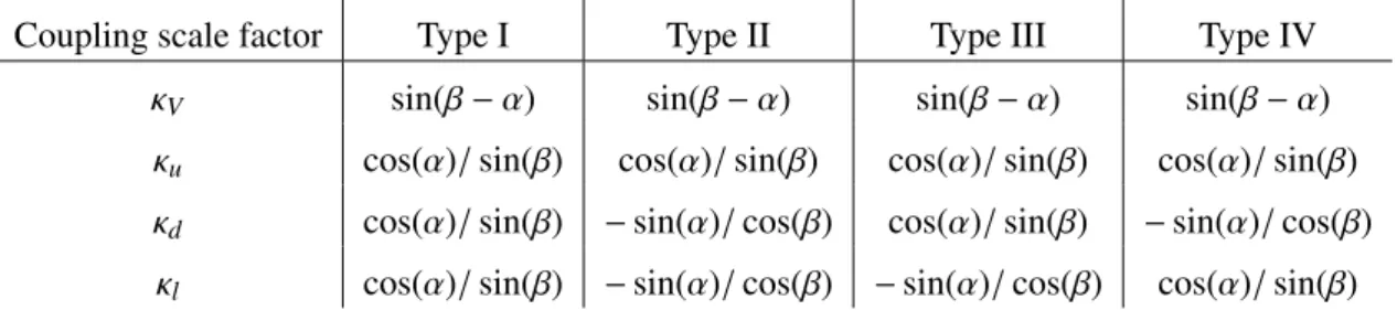
The Glashow-Weinberg condition is satisfied by four types of 2HDMs [38]:

•

Type I: One Higgs doublet couples to vector bosons, while the other couples to fermions. The first doublet is “fermiophobic” in the limit of no mixing.

•

Type II: This is an “MSSM-like” model, in which one Higgs doublet couples to up-type quarks and the other to down-type quarks and leptons.

•

Type III: This is a “lepton-specific” model, where the Higgs bosons have the same couplings to quarks as in the Type I model and to leptons as in Type II.

•

Type IV: This is a “flipped” model, where the Higgs bosons have the same couplings to quarks as

in the Type II model and to leptons as in Type I.

6 TWO-HIGGS-DOUBLET MODEL

9

Coupling scale factor Type I Type II Type III Type IV

κ

sin(β

α) sin(β

α) sin(β

α) sin(β

α)

κ

cos(α)/ sin(β) cos(α)/ sin(β) cos(α)/ sin(β) cos(α)/ sin(β) κ

cos(α)/ sin(β)

sin(α)/ cos(β) cos(α)/ sin(β)

sin(α)/ cos(β)

κ

cos(α)/ sin(β)

sin(α)/ cos(β)

sin(α)/ cos(β) cos(α)/ sin(β)

Table 2: Couplings of the light Higgs boson h to weak vector bosons (κ

), up-type quarks (κ

), down- type quarks (κ

), and leptons (κ

), expressed as ratios to the corresponding SM predictions in 2HDMs of various types.

The couplings of the light Higgs boson h to vector bosons and fermions in each of the four types of 2HDMs, expressed as ratios relative to the Higgs boson couplings in the SM, are summarized in Ta- ble 2 [41]. The coupling scale factors are denoted κ

for the W and Z bosons, κ

for up-type quarks, κ

for down-type quarks, and κ

for charged leptons.

The Higgs boson rate measurements in different production and decay modes are interpreted in each of these four types of 2HDMs assuming that the observed new particle with mass m

125.5 GeV is the light CP-even neutral Higgs boson h. This is done by rescaling the production and decay rates as functions of the couplings κ

, κ

, κ

, and κ

. The measurements of ratios of these couplings, which assume the same production modes as in the SM but do not make any assumption about the Higgs boson total width, are given in Models 3 and 4 of Table 1. These couplings are in turn expressed as a function of the underlying parameters, the two angles β and α, using the relations shown in Table 2. Here it is also assumed that the decay modes are the same as those for the SM Higgs boson.

The coupling-rescaled predictions agree with those obtained using the

[42] and

[43]

programs, which calculate Higgs boson production and decay rates respectively in two-Higgs-doublet models. The rescaled gluon fusion rate agrees with the

prediction well within a percent, and the rescaled decay rates show a similar level of agreement. The cross section for bbh associated production is calculated using

and included as a correction that scales with the square of the Yukawa coupling to the b-quark, under the assumption that it produces differential distributions that are the same as those in gluon fusion. The correction is generally below 10% of the total production rate for the regions of parameter space compatible with data at 95% CL.

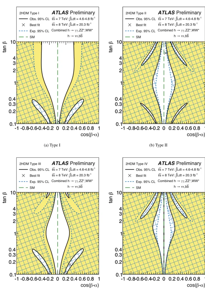
Figure 4 shows the regions of the (cos(β

α), tan β) plane that are excluded at 95% CL or greater for each of the four types of 2HDMs, overlaid with the expected exclusion limits obtained by assuming the SM Higgs sector. The observed and expected exclusion regions in cos(β

α) depend on the particular functional dependence of the couplings on β and α, which are different for each of the four types of 2HDMs as shown in Table 2. There is a physical boundary κ

1 in all four 2HDM types, so the profile likelihood ratio is restricted to the physical region

sin(β

α)| ≤ 1. The data are consistent with the SM- like alignment limit at cos(β

α)

0 within

in each of the models. The range 0.1≤ tan β

shown as only that part of the parameter space was scanned in the present version of this analysis. The compatible region extends to larger and smaller tan β values, but with a correspondingly narrower range of cos(β

α).

The confidence intervals drawn in Fig. 4 assume a χ

distribution with two parameters of interest.

However, at cos(β

α)

0 the likelihood is independent of the model parameter β, e

ectively reducing

the number of parameters of interest locally to one. Hence the assumed test statistic distribution for two

parameters of interest leads to some overcoverage near cos(β

α)

0.

6 TWO-HIGGS-DOUBLET MODEL

10

α) β- cos(

βtan

0.1 0.2 0.3 0.4 1 2 3 4 10

-1 -0.8-0.6-0.4-0.2 0 0.2 0.4 0.6 0.8 1

βtan

0.1 0.2 0.3 0.4 1 2 3 4 10

-1 -0.8-0.6-0.4-0.2 0 0.2 0.4 0.6 0.8 1 ATLAS Preliminary

Ldt = 4.6-4.8 fb-1

∫

= 7 TeV:

s

Ldt = 20.3 fb-1

∫

= 8 TeV:

s

,ZZ*,WW*

γ γ

→ Combined h

b τ,b τ h → Combined Obs. 95% CL

Best fit Exp. 95% CL SM 2HDM Type I

(a) Type I

α) β- cos(

βtan

0.1 0.2 0.3 0.4 1 2 3 4 10

-1 -0.8-0.6-0.4-0.2 0 0.2 0.4 0.6 0.8 1

βtan

0.1 0.2 0.3 0.4 1 2 3 4 10

-1 -0.8-0.6-0.4-0.2 0 0.2 0.4 0.6 0.8 1 ATLAS Preliminary

Ldt = 4.6-4.8 fb-1

∫

= 7 TeV:

s

Ldt = 20.3 fb-1

∫

= 8 TeV:

s

,ZZ*,WW*

γ γ

→ Combined h

b τ,b τ h → Combined Obs. 95% CL

Best fit Exp. 95% CL SM 2HDM Type II

(b) Type II

α) β- cos(

βtan

0.1 0.2 0.3 0.4 1 2 3 4 10

-1 -0.8-0.6-0.4-0.2 0 0.2 0.4 0.6 0.8 1

βtan

0.1 0.2 0.3 0.4 1 2 3 4 10

-1 -0.8-0.6-0.4-0.2 0 0.2 0.4 0.6 0.8 1 ATLAS Preliminary

Ldt = 4.6-4.8 fb-1

∫

= 7 TeV:

s

Ldt = 20.3 fb-1

∫

= 8 TeV:

s

,ZZ*,WW*

γ γ Combined h →

b ,b τ τ

→ h Combined Obs. 95% CL

Best fit Exp. 95% CL SM 2HDM Type III

(c) Type III

α) β- cos(

βtan

0.1 0.2 0.3 0.4 1 2 3 4 10

-1 -0.8-0.6-0.4-0.2 0 0.2 0.4 0.6 0.8 1

βtan

0.1 0.2 0.3 0.4 1 2 3 4 10

-1 -0.8-0.6-0.4-0.2 0 0.2 0.4 0.6 0.8 1 ATLAS Preliminary

Ldt = 4.6-4.8 fb-1

∫

= 7 TeV:

s

Ldt = 20.3 fb-1

∫

= 8 TeV:

s

,ZZ*,WW*

γ γ Combined h →

b ,b τ τ

→ h Combined Obs. 95% CL

Best fit Exp. 95% CL SM 2HDM Type IV

(d) Type IV

Figure 4: Regions of the (cos(β−α), tan β) plane of four types of 2HDMs excluded by fits to the measured

rates of Higgs boson production and decays. The likelihood contours where

6.0, corresponding

approximately to 95% CL (2σ), are indicated for both the data and the expectation assuming the SM

Higgs sector. The cross in each plot marks the observed best-fit value. The light shaded and hashed

regions indicate the observed and expected exclusions, respectively.

7 SIMPLIFIED MSSM

11

7 Simplified MSSM

Supersymmetry [44–52] provides a means to solve the hierarchy problem by introducing superpartners whose radiative corrections to the Higgs boson mass cancel those of the corresponding SM particles.

Many supersymmetric models also provide a candidate for a dark matter particle.

In the Minimal Supersymmetric Standard Model [53–57], the mass mixing matrix for the neutral, CP-even Higgs bosons is:

M²_S =

(m

δ

)











cos

(β)

cos(β) sin(β)

−

cos(β) sin(β) sin

(β)









 +

m











sin

(β)

cos(β) sin(β)

−

cos(β) sin(β) cos

(β)









 +













0 0

0

sin²(β)













(15) where δ

and δ are radiative corrections involving primarily top quarks and stops. The couplings in a simplified MSSM model can be obtained from this mass mixing matrix as follows [58, 59].

The trace of the mass mixing matrix is taken and evaluated at the light Higgs boson mass of m

125.5 GeV, allowing the δ

and δ corrections to be determined as a function of m

and tan β. Neglecting the sub-leading correction δ

, then by substituting for δ the mass mixing matrix is fully determined by m

and tan β. This matrix is diagonalized to find the eigenvectors, and in particular those components of the eigenvector corresponding to the light Higgs boson, s

and s

. This allows the Higgs boson couplings to vector bosons (κ

), up-type fermions (κ

), and down-type fermions (κ

), as ratios to the corresponding SM expectations, to be determined as functions of m

and tan β only:

κ

1+tan²β

κ

s

(m

, tan β)

√

1+tan²β tanβ

κ

s

(m

, tan β)

1

tan

β,

(16)

where the functions s

and s

are given by:

s

1+

(

)

(

Atan2β−m2

h

(

))

s

(

Z

)

m²

Z+m²

Atan²β−m²

h

(

) s

.

(17)

To test this model, the measured production and decay rates are expressed in terms of the correspond- ing couplings. Model 3 of Table 1 lists the measurements of ratios of the κ

, κ

, and κ

couplings. These are measured assuming identical production modes to the SM, but without any assumption about the Higgs boson total width. The couplings are in turn cast in terms of m

and tan β using Eq. 16, with the additional assumption that the decay modes are the same as those for the SM Higgs boson. A correction is applied for bbh associated production as a function of the b-quark Yukawa coupling as described in Sec. 6. Loop corrections from stops in gluon fusion production and diphoton decays are expected to be small – less than about 5% for m

> 500 GeV [58] – and are neglected. Additional corrections in the MSSM that would break the universality of down-type fermion couplings, such that for example κ

κ

, are generally sub-dominant effects [59] and are not included.

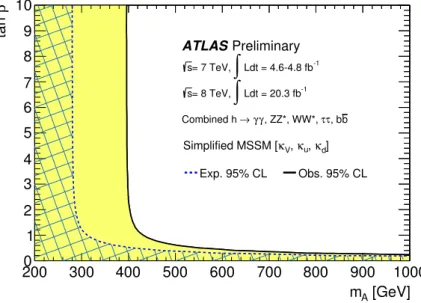
The two-dimensional likelihood scan in the (m

, tan β) plane for this simplified MSSM model is

shown in Fig. 5. The data are consistent with the SM decoupling limit at large m

. The observed

(expected) lower limit at 95% CL on the CP-odd Higgs boson mass is m

> 400 GeV (280 GeV)

8 HIGGS PORTAL TO DARK MATTER

12

[GeV]

mA

200 300 400 500 600 700 800 900 1000

βtan

0 1 2 3 4 5 6 7 8 9 10

Preliminary ATLAS

Ldt = 4.6-4.8 fb-1

∫

= 7 TeV, s

Ldt = 20.3 fb-1

∫

= 8 TeV, s

b τ, b τ , ZZ*, WW*, γ

γ

→ Combined h

d] κ

u, κ

V, κ Simplified MSSM [

Exp. 95% CL Obs. 95% CL

Figure 5: Regions of the (m

, tan β) plane excluded in a simplified MSSM model via fits to the measured rates of Higgs boson production and decays. The likelihood contours where

6.0, corresponding approximately to 95% CL (2σ), are indicated for the data and expectation assuming the SM Higgs sector.

The light shaded and hashed regions indicate the observed and expected exclusions, respectively. The SM decoupling limit is m

for 2

tan β

10, with the limit increasing to larger masses for tan β < 2. The observed limit is stronger than expected since the measured rates in the h

γγ (expected to be dominated by a W boson loop) and h

ZZ

4` channels are higher than predicted by the SM, but the simplified MSSM has a physical boundary κ

1 so the vector boson coupling cannot be larger than the SM value. The physical boundary is accounted for by computing the profile likelihood ratio with respect to the maximum likelihood obtained within the physical region of the parameter space, m

>0 and tan β >0. The range 0≤ tan β

analysis. The compatible region extends to larger tan β values.

The results reported here pertain to the simplified MSSM model studied and are not fully general.

The MSSM includes other possibilities such as Higgs boson decays to supersymmetric particles, decays of heavy Higgs bosons to lighter ones, and effects from light supersymmetric particles [60] which are not investigated here.

8 Higgs Portal to Dark Matter

Many “Higgs portal” models [14, 34, 61–65] introduce an additional weakly-interacting massive particle (WIMP) as a dark matter candidate. It is assumed to interact very weakly with the SM particles, except for the Higgs boson. In this study, the coupling of the Higgs boson to the WIMP is taken to be a free parameter.

The upper limit on the branching ratio of the Higgs boson to invisible final states, BR

, is derived

using the combination of rate measurements from the h

γγ, h

ZZ

4`, h

WW

`ν`ν,

h

ττ, and h

b b ¯ channels, together with the measured upper limit on the rate of the Zh

``

E

process. The couplings of the Higgs boson to massive particles other than the WIMP are assumed to be

equal to the SM predictions, allowing the corresponding partial decay widths and invisible decay width

8 HIGGS PORTAL TO DARK MATTER

13 to be inferred. Effective couplings to photons, κ

, and gluons, κ

, are introduced to absorb the possible contributions of new particles through loops. The Higgs boson production modes are assumed to be the same as those in the SM.

The ratio of the total width of the Higgs boson to the SM expectation,

/

, is parametrized by κ

such that:

κ

/

i

κ

/(1

BR

)

i

κ

0.0023 κ

0.085 κ

0.91,

(18)

where the branching ratios of a Higgs boson with m

125.5 GeV to photons and gluons are 0.0023 and 0.085 respectively, and 0.91 is the sum of the branching ratios of the Higgs boson to massive parti- cles [25]. Thus the production and decay rates of all channels are fit with functions of κ

, κ

, and BR

. The photon and gluon couplings are treated as nuisance parameters.

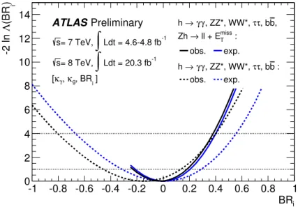
The resulting likelihood scan as a function of BR

is shown in Fig. 6. There is a lower physical boundary such that BR

0, with the SM corresponding to BR

0. Ignoring this boundary, the branching ratio of the Higgs boson to invisible final states is measured to be BR

0.20 with the combination of all channels, while the expected value is 0.00

0.21. If data from the Zh

``

E

search is not included, the measured (expected) value is BR

(0.00

) [13]. The measurements for the [κ

, κ

, BR

] parametrization used are listed in Models 6 and 7 of Table 1.

The best-fit value for BR

is negative because the Higgs boson couplings to massive particles are assumed to be equal to the SM values, so the measured overall µ

>1 is accommodated in the fit by decreasing the Higgs boson total width. The smaller expected uncertainty when including the Zh

``

E

channel demonstrates the increase in sensitivity. Accounting for the boundary produces an observed (expected) 95% CL upper limit of BR

< 0.37 (0.39) using the combination of all channels.

The observed (expected) upper limit without including the Zh

``

E

data is BR

< 0.41 (0.55).

To compare with direct searches for dark matter, the observed upper limit BR

< 0.37 obtained by combining all channels is translated into constraints on the coupling of the WIMP to the Higgs boson as a function of its mass [63]. It is assumed that the WIMP mass is less than half the Higgs boson mass and that the resulting Higgs boson decays to WIMP pairs account entirely for BR

. These assumptions produce conservative limits as any additional contributions to BR

from other new phenomena would produce more stringent results. The partial width for Higgs boson decays to a pair of dark matter particles depends on the spin of the dark matter particle. It is given for scalar, Majorana fermion, or vector dark matter candidates (where the Majorana fermion is motivated by neutralinos in supersymmetry) as:

scalar S :

(h

S S )

λ

v

β

128πm

fermion f :

(h

f f )

λ

v

β

m

64π vector V :

(h

VV)

λ

v

β

m

512πm









1

4 m

m

12 m

m









.

(19)

Here λ

, λ

/

, and λ

are the couplings of the Higgs boson to dark matter particles of correspond- ing spin, v

246 GeV denotes the vacuum expectation value of the Higgs boson, and β

1

4m

/m

is a kinematic factor associated with the two-body h

χχ decay. These equations are used to deduce the coupling of the Higgs boson to the WIMP for each of the three possible WIMP spins.

The coupling is then re-parametrized in terms of the cross section for scattering between the WIMP

9 CONCLUSIONS

14

BRi

-1 -0.8 -0.6 -0.4 -0.2 0 0.2 0.4 0.6 0.8 1 ) i(BRΛ-2 ln

0 2 4 6 8 10 12

14 ATLAS Preliminary

Ldt = 4.6-4.8 fb-1

∫

= 7 TeV, s

Ldt = 20.3 fb-1

∫

= 8 TeV, s

i ]

g, BR , κ κγ

[

: b τ, b , ZZ*, WW*, τ γ

γ h →

, b τ, b , ZZ*, WW*, τ γ

γ h →

T : ll + Emiss

→ Zh

obs. exp.

obs. exp.

Figure 6: Likelihood scan of the invisible branching ratio of the Higgs boson, BR

, where the effective loop-induced couplings to photons, κ

, and gluons, κ

, have been profiled. The observed and expected likelihoods are each shown with and without the inclusion of the Zh

``

E

channel. Ignoring the physical boundary BR

0, the lines at

1.0 and

4.0 correspond approximately to 68% CL (1σ) and 95% CL (2σ), respectively.

and nucleons via Higgs boson exchange, σ

[63]:

scalar S : σ

λ

m

f

16πm

(m

m

)

fermion f : σ

λ

Λ²

m

f

m

4πm

(m

m

)

vector V : σ

λ

m

f

16πm

(m

m

)

,

(20)

where m

0.94 GeV is the nucleon mass, and f

0.33

is the form factor associated with the Higgs-nucleon coupling, computed using lattice QCD [63].

Upper limits at 95% CL on the WIMP-nucleon scattering cross section σ

are derived as a function of the WIMP mass m

(χ

S , V, or f ), as shown in Fig. 7. They are compared with limits from direct searches for dark matter [66–72] at the confidence levels indicated. The ATLAS limits on the WIMP- nucleon scattering cross section are proportional to those on BR

. They are considerably more stringent at low mass and degrade as m

approaches m

/2 as expected from kinematics. The limits are shown for m

1 GeV, but extend to smaller WIMP masses than this value.

9 Conclusions

Higgs boson coupling measurements from the combination of multiple production and decay channels

(h

γγ, h

ZZ

4`, h

WW

`ν`ν, h

ττ, and h

b b), along with a search for invisible ¯

decays of the Higgs boson (Zh

``

E

), have been used to search indirectly for new physics. The

9 CONCLUSIONS

15

[GeV]

mχ

1 10 10² 10³

]2 [cm -Nχσ

10-57

10-55

10-53

10-51

10-49

10-47

10-45

10-43

10-41

10-39

DAMA/LIBRA (99.7% CL) CRESST (95% CL) CDMS (95% CL) CoGeNT (90% CL) XENON10 (90% CL) XENON100 (90% CL) LUX (95% CL)

Scalar WIMP Majorana WIMP Vector WIMP

ATLAS Preliminary

Higgs portal model:

ATLAS (95% CL) in dt = 4.6-4.8 fb-1

∫

dt = 20.3 fb-1

∫

ν, νl

→l

→WW*

4l, h

→

→ZZ*

γ, h γ

→ h

miss

ll+ET

→ bb, Zh

→ τ, h τ

→ h

Figure 7: ATLAS upper limit at 95% CL on the WIMP-nucleon scattering cross section in a Higgs portal

model as a function of the mass of the dark matter particle, shown separately for a scalar, Majorana

fermion, or vector boson WIMP. The hashed bands indicate the uncertainty resulting from the form

factor f

. Excluded and allowed regions from direct detection experiments at the confidence levels

indicated are also shown [66–72]. These are spin-independent results obtained directly from searches

for nuclei recoils from elastic scattering of WIMPs, rather than being inferred indirectly through Higgs

boson exchange in the Higgs portal model.

9 CONCLUSIONS

16 results are based on up to 4.8 fb

of pp collision data at

s

7 TeV and 20.3 fb

at

s

8 TeV

recorded by the ATLAS experiment at the LHC. No evidence for physics beyond the Standard Model

is observed. The mass dependence of the couplings is consistent with the predictions for a SM Higgs

boson. Constraints are set on minimal Higgs compositeness models, an additional electroweak singlet,

two-Higgs-doublet models, a simplified MSSM, and a Higgs portal to dark matter.

REFERENCES

17

References

[1] ATLAS Collaboration, Observation of a new particle in the search for the Standard Model Higgs boson with the ATLAS detector at the LHC, Phys. Lett.

(2012) 1, arXiv:1207.7214 [hep-ex].

[2] CMS Collaboration, Observation of a new boson at a mass of 125 GeV with the CMS experiment at the LHC, Phys. Lett.

(2012) 30, arXiv:1207.7235 [hep-ex].

[3] ATLAS Collaboration, Measurements of Higgs boson production and couplings in diboson final states with the ATLAS detector at the LHC, Phys. Lett.

(2013) 88, arXiv:1307.1427 [hep-ex].

[4] CMS Collaboration, Combination of standard model Higgs boson searches and measurements of the properties of the new boson with a mass near 125 GeV, CMS-PAS-HIG-13-005 (2013).

https://cds.cern.ch/record/1542387.

[5] ATLAS Collaboration, Evidence for the spin-0 nature of the Higgs boson using ATLAS data, Phys.

Lett.

(2013) 120, arXiv:1307.1432 [hep-ex].

[6] CMS Collaboration, Study of the Mass and Spin-Parity of the Higgs Boson Candidate Via Its Decays to Z Boson Pairs, Phys. Rev. Lett.

(2013) 081803, arXiv:1212.6639 [hep-ex].

[7] CMS Collaboration, Measurement of the properties of a Higgs boson in the four-lepton final state, arXiv:1312.5353 [hep-ex].

[8] F. Englert and R. Brout, Broken symmetry and the mass of gauge vector mesons, Phys. Rev. Lett.

13

(1964) 321.

[9] P. W. Higgs, Broken symmetries and the masses of gauge bosons, Phys. Rev. Lett.

(1964) 508.

[10] G. Guralnik, C. Hagen, and T. Kibble, Global conservation laws and massless particles, Phys.

Rev. Lett.

(1964) 585.

[11] ATLAS Collaboration, Evidence for Higgs Boson Decays to the τ

τ

Final State with the ATLAS Detector, ATLAS-CONF-2013-108 (2013). https://cds.cern.ch/record/1632191.

[12] ATLAS Collaboration, Search for the bb decay of the Standard Model Higgs boson in associated W

ZH production with the ATLAS detector, ATLAS-CONF-2013-079 (2013).

https://cds.cern.ch/record/1563235.

[13] ATLAS Collaboration, Updated coupling measurements of the Higgs boson with the ATLAS detector using up to 25 fb

of proton-proton collision data, ATLAS-CONF-2014-009 (2014).

https://cds.cern.ch/record/1670012.

[14] ATLAS Collaboration, Search for Invisible Decays of a Higgs Boson Produced in Association with a Z Boson in ATLAS, arXiv:1402.3244 [hep-ex].

[15] ATLAS Collaboration, Combined search for the Standard Model Higgs boson in pp collisions at

√

s

7 TeV with the ATLAS detector, Phys. Rev.

(2012) 032003, arXiv:1207.0319 [hep-ex].

[16] ATLAS and CMS Collaborations, Procedure for the LHC Higgs boson search combination in Summer 2011, ATL-PHYS-PUB-2011-011, CERN-CMS-NOTE-2011-005 (2011).

http://cdsweb.cern.ch/record/1375842.