ATLAS-CONF-2013-027 11March2013
ATLAS NOTE
ATLAS-CONF-2013-027
March 10, 2013
Search for Higgs bosons in Two-Higgs-Doublet models in the H → WW → eνµν channel with the ATLAS detector
The ATLAS Collaboration
Abstract
The Higgs-like boson observed at the LHC with a mass of approximately 125 GeV could
be part of an extended scalar sector originating from two complex Higgs doublets. The
analysis presented in this note investigates the possibility of a Two-Higgs-Doublet model
(2HDM) being realized in nature by searching for evidence of a second, heavier, CP-even
scalar boson in the
H→WW(∗) →e−ν¯
eµ+νµ/e+νeµ−ν¯
µdecay mode. The analysis is based
on proton-proton collision data at a centre-of-mass energy of 8 TeV collected with the AT-
LAS detector and corresponding to an integrated luminosity of 13.0 fb
−1. Artificial neural
network techniques are used to maximise the sensitivity. No evidence for a second scalar
boson is found in the investigated mass range between 135 and 300 GeV. Exclusion limits
on type-I and type-II 2HDMs are set as a function of the two mixing angles
αand
βas well
as the mass
mHof the heavier scalar boson. For the limits the signal hypothesis includes the
Higgs-like boson at 125 GeV and assumes that it is the light scalar
hof a 2HDM, while the
null hypothesis assumes no Higgs boson at all.
1 Introduction
The experiments ATLAS and CMS at the Large Hadron Collider (LHC) have observed a Higgs-like boson at a mass of approximately 125 GeV [1, 2]. To-date, all measurements concerning the production rates, the branching ratios and kinematic distributions are compatible with this particle being the Higgs boson predicted by the Standard Model (SM). The mass of the observed state is also consistent with constraints on the Higgs boson mass obtained from electroweak precision measurements [3].
The so-called Brout-Englert-Higgs (BEH) mechanism [4, 5, 6] implements the spontaneous breaking of the electroweak gauge symmetry and thereby explains the mass generation of elementary particles, in particular the mass of the weak gauge bosons, but also the mass of the fermions via the Yukawa coupling.
The resulting field and the associated Higgs boson are essential to formulate a consistent and coherent theory of electroweak interactions.
The BEH mechanism of the SM postulates the existence of one doublet of complex fields, yielding four degrees of freedom, three of which provide the longitudinal polarisation modes of the massive weak gauge bosons, while one degree of freedom materialises as the Higgs boson. In this form the SM BEH mechanism constitutes only a minimal configuration to implement the breaking of the electroweak symmetry and the generation of particle masses. A simple extension of the SM Higgs sector is given by the addition of a second complex Higgs doublet [7], giving rise to five Higgs bosons: two CP-even scalar fields h and H, one pseudoscalar A (CP-odd), and two charged fields H
±. These Two-Higgs-Doublet models (2HDM) are phenomenologically interesting since they can explain the generation of the baryon asymmetry in the universe [8] and are an important ingredient of axion models that are designed to explain its the dark matter content [9]. Finally, the minimal supersymmetric SM [10] contains two Higgs doublets as well. Four different types of 2HDMs can be distinguished, depending on the different coupling of the two scalar fields h and H to fermions and weak gauge bosons. In type-I models all quarks couple to just one of the Higgs doublets, while in type-II models the right-handed up-type quarks couple to one Higgs doublet and the right-handed down-type quarks to the other doublet. Type-III and type-IV models differ only from type-I and type-II models in their couplings to the leptons. Since the analysis presented in this note is not sensitive to the leptonic couplings, type-III and type-IV models are not considered. Recent detailed reviews on 2HDMs can be found in Refs. [11, 12]. Since the discovery of the Higgs-like boson at the LHC, 2HDMs have attracted much attention in phenomenological studies [13, 14, 15, 16, 17], which provide a strong incentive for dedicated experimental investigations in this direction.
Searches for generic 2HDMs have been performed by the CDF collaboration at the Tevatron [18, 19].
The rate of the Higgs-like boson at 125 GeV in the two-photon channel provides also constraints on 2HDMs [20], mainly reducing the parameter space of type-II models.
The analysis presented in this note investigates the possibility that the boson observed by the ATLAS and CMS experiments at a mass of 125 GeV originates from a Higgs boson that is part of a 2HDM. In particular, it is assumed that the observed particle is the low mass Higgs h of the 2HDM. The analysis searches for additional signal contributions by the higher mass CP-even boson H of the model. Both Higgs bosons are reconstructed in the h
/H
→WW
(∗) →e
−ν¯
eµ+νµ/e
+νeµ−ν¯
µdecay channel and their contributions are both part of the signal hypothesis, while the null hypothesis assumes no Higgs boson at all. The pseudoscalar A does not decay to pairs of vector bosons and therefore does not contribute to the signal rates directly. Indirect contributions, for example via A
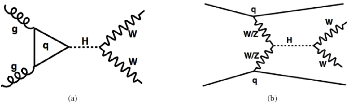
→τ+τ−decays, are neglected, which leads to a slight underestimation of the sensitivity. The following two production modes of Higgs bosons are considered: the gluon fusion process, see Fig. 1(a) and the vector-boson-fusion (VBF) process, see Fig. 1(b). To be sensitive to both production mechanisms the analysis considers two different final states.
In the first channel, two charged leptons and large missing transverse momentum E
Tmissare required (0-
jet channel), and in the second channel, which is sensitive to the VBF process, two high-p
Tjets (2-jet
channel) are reconstructed in addition.
(a) (b)
Figure 1: Leading order Feynman diagrams for Higgs boson production via (a) gluon fusion and (b) vector boson fusion (VBF).
The expected signal rates depend on the mixing angles
αand
βof the two Higgs doublets and the mass m
Hof the higher mass state H. Different signal hypotheses characterized by different values of cos
α,tan
β, andm
Hare tested using the CLs method. Artificial neural networks (NN) are used to enhance the sensitivity by combining the information contained in various kinematic and angular variables. The mass interval of 135
<m
H<300 GeV is probed in the hypothesis tests.
2 Data samples and samples of simulated events
The analysis described in this note uses LHC pp collision data at a centre-of-mass energy of 8 TeV collected with the ATLAS detector [21] between April and September 2012. The selected events were recorded based on single-electron and single-muon triggers. Stringent detector and data quality require- ments are applied, resulting in a dataset corresponding to an integrated luminosity of 13.0 fb
−1.
The ATLAS detector is built from a set of cylindrical subdetectors, which cover almost the full solid angle
1around the interaction point.
ATLAS is composed of an inner tracking system close to the interaction point, surrounded by a super- conducting solenoid providing a 2 T axial magnetic field, electromagnetic and hadronic calorimeters, and a muon spectrometer. The electromagnetic calorimeter is a lead liquid-argon sampling calorimeter (LAr) with high granularity. An iron-scintillator tile calorimeter provides hadronic energy measurements in the central pseudorapidity range. The endcap and forward regions are instrumented with LAr calorimeters for both electromagnetic and hadronic energy measurements. The muon spectrometer consists of three large superconducting toroids, a system of trigger chambers, and precision tracking chambers.
In the analysis, the production of the two CP-even Higgs bosons h and H of the 2HDM is modelled with samples of simulated events generated for SM Higgs boson studies, while scaling the production cross sections according to the parameters of the 2HDM. The mass of the light Higgs boson h is fixed to m
h=125 GeV in simulation. The mass of the heavy Higgs boson H is varied between 135 and 300 GeV, using steps of 5 GeV between 135 and 200 GeV and steps of 20 GeV between 200 and 300 GeV. In the search region, the natural width of the Higgs bosons is negligible with respect to the experimental resolution. The samples of simulated events for the Higgs boson gluon fusion and the VBF processes are generated with the POWHEG [22, 23] package, interfaced to PYTHIA [24] for showering and hadroni- sation. The associated W H and ZH production processes are modelled using PYTHIA, with the Higgs boson decaying to W
+W
−, while the W and Z bosons decay inclusively to all modes. At particle level
1ATLAS uses a right-handed coordinate system with its origin at the nominal interaction point in the centre of the detector and thez-axis along the beam direction. Thez-axis is parallel to the anti-clockwise beam viewed from above. The pseudora- pidityηis defined asη=−ln[tan(θ/2)], where the polar angleθis measured with respect to thez-axis. The azimuthal angleφ
an event filter is applied that requires two charged leptons from the decay of the Higgs boson. The CT10 [25] set of parton distribution functions (PDF) is used for the gluon-fusion, the VBF, and the W H/ZH samples.
The cross section of the gluon-fusion process has been computed with next-to-next-to-leading order (NNLO) QCD corrections [26, 27, 28], next-to-leading order (NLO) electroweak corrections [29, 30], and corrections arising from the resummation of soft-gluon terms [31]. When rescaling the SM gluon- fusion cross section to a specific 2HDM, the different scaling of the top-quark-loop and bottom-quark- loop contributions, as well as their interference, is properly accounted for by using calculations that provide the relevant split of these three contributions [32, 33]. The expectation value of VBF Higgs boson events is computed by using theoretical cross-section predictions that include full NLO QCD and electroweak corrections [34, 35, 36] and approximate NNLO QCD corrections [37]. The theoretical cross-sections for the Higgs-strahlung processes W H and ZH are calculated with NNLO QCD correc- tions [38] and NLO electroweak corrections [39].
Inclusive W and Z/γ
∗vector boson production in association with jets is simulated using the leading- order (LO) generator ALPGEN version 2.13 [40], showered with HERWIG [41] in connection with the JIMMY [42] underlying event model. W+jets and Z+jets events with up to five additional partons are generated. The MLM matching scheme [43] is used to remove jets generated by the parton shower and those from the matrix element.
The diboson processes (WW , WZ, Wγ
∗, and ZZ) are generated using POWHEG and showered with PYTHIA. An additional contribution to the continuum WW background from gluon-initiated diagrams is modelled using gg2WW [44], also interfaced to HERWIG and JIMMY. The matrix element generators MADGRAPH [45] and ALPGEN (interfaced to HERWIG) are used to model Wγ
∗with m
γ∗ <7 GeV and Wγ, respectively. Samples of the t-channel single top-quark process are produced with the A
cerMC program [46] linked to PYTHIA [24] for showering and hadronisation. The s-channel single top-quark process and Wt production are generated using MC@NLO version 3.41 [47] and showered with HER- WIG. Samples modelling t t ¯ pair production are generated with MC@NLO. All top-quark processes are produced with a top-quark mass of 172.5 GeV.
More details on the event generators applied in this analysis and on the theoretical cross-sections used to normalise these samples can be found in Ref. [48], describing the SM Higgs boson analysis in the H
→WW
∗channel.
After the event generation step, all samples are passed through the full simulation of the ATLAS detector [49] based on GEANT4 [50] and are then reconstructed using the same procedure as for collision data. The simulation includes the effect of multiple pp collisions per bunch crossing (pile-up) at a variable rate and the events are weighted to match the conditions of the data sample using the average number of collisions per bunch crossing.
3 Object definitions and event selection
Candidate events of the h/H
→WW
(∗) →eνµν process are recorded using unprescaled single-electron and single-muon triggers with a p
Tthreshold of 24 GeV. A number of requirements are applied in order to ensure a consistent event quality and to remove mis-reconstructed events. Events are selected if they contain at least one good primary vertex candidate with at least three associated tracks with p
T >0.4 GeV. Non-collision backgrounds are excluded, i.e. cosmic rays passing through the detector, beam backgrounds and instrumental effects like noise bursts in certain parts of the detector. The event selection is based on the identification of electrons, muons and jets and on the reconstruction of E
missT(missing transverse momentum).
Electron candidates are selected from LAr electromagnetic calorimeter clusters matched to tracks and
are reconstructed offline using a Gaussian sum filter algorithm [51]. The energy of an electron candidate
is taken from the calorimeter cluster, while its
ηand
φare taken from the track. It is required that the track points back to the primary vertex with transverse impact parameter significance (the ratio of the transverse impact parameter to its error) less than 3. The z-position of the track has to be compatible with the primary vertex. Electron candidates are excluded if they lie in the pseudorapidity ranges 1.37<
|η| <1.52 or|η| >2.47. The electron candidates are further required to fulfil stringent criteria regarding
calorimeter shower shape, track quality, track-cluster matching, and transition radiation energy to ensure high identification quality. Electron candidates are required to be isolated by placing cuts on
Σ(ptrackT), the scalar sum of the transverse momenta of tracks in a cone of
∆R = p∆η2+ ∆φ2 =
0.3 around the candidate excluding the track associated to the electron candidate, and
Σ(p
caloT), the scalar sum of the transverse momenta of calorimeter energy deposits for a cone of the same size also excluding the energy deposit associated to the candidate. For an electron candidate the fractional track based isolation,
Σ(ptrackT)/p
Tis required to be below 0.16, and this is tightened to 0.12 for candidates with p
Tbelow 25 GeV which have more background, while
Σ(p
caloT)/ p
Tis required to be below 0.16. If two electron candidates are reconstructed within a cone of
∆R=0.1, the candidate the with lower p
Tis discarded.
Muons are reconstructed by taking a statistical combination of the matched tracks in the Inner De- tector (ID) and in the Muon Spectrometer (MS). The muon candidates are required to have a sufficiently large number of hits in the silicon detector and the Transition Radiation Tracker (TRT). Muon tracks are required to have at least one hit in the pixel detector, and four or more hits in the Semiconductor Tracker (SCT). Tracks are vetoed if they have more than two missing hits in the SCT and pixel detectors, as well as tracks with an excessive number of outlier hits in the TRT. The momentum as measured using the ID is required to agree with the momentum measured using the MS after correcting for the predicted muon energy loss in the calorimeter. Muon candidates are required to have p
T >15 GeV and
|η| <2.4, and must satisfy a similar isolation and the same impact parameter cuts as electron candidates. The required calorimeter isolation is
Σ(pcaloT)/p
T <0.014/GeV
·p
T−0.15 and
Σ(p
caloT)/p
T <0.20, while for the track based isolation
Σ(p
trackT)/ p
T <0.01/GeV
·p
T−0.105 and
Σ(ptrackT)/p
T <0.15 is required. If an electron lies in a cone of
∆R=0.1 around a reconstructed muon, the electron candidate is ignored.
The reconstruction, identification and trigger efficiencies of electrons and muons were measured using tag-and-probe methods on samples enriched with Z
→ ℓℓ,J/ψ
→ ℓℓ, orW
± → ℓν(ℓ
=e, µ) events.
Jets are reconstructed from topological clusters using the anti-k
talgorithm [52] with the size pa- rameter R
=0.4. The response of the calorimeter is corrected through a p
T- and
η-dependent factor,which is derived from simulated events and is applied to each jet to provide an average energy scale correction [53]. The selected jets are required to have p
T >25 GeV at the hadronic energy scale. This threshold is increased to 30 GeV in the forward region (
|η|>2.5) which is more sensitive to reconstruc- tion issues arising from pile-up events. Only jets within
|η| <4.5 are used. To reject jets from pile-up events, a quantity called the jet-vertex fraction (JVF) is defined as the ratio of
Pp
Tfor all tracks within the jet that originate from the primary vertex associated to the hard-scattering collision to the
Pp
Tof all tracks matched to the jet; and it is required that JVF
>0.5. For jets having no matched tracks, this criteria is omitted. Selected jets are identified as b-quark jets by reconstructing secondary and tertiary vertices from the tracks associated with each jet and combining lifetime related information with a NN [54]. The identification requirement has an efficiency of 85% for b-quark jets in t t ¯ events. If a jet candidate lies within a cone of
∆R=0.3 around a reconstructed electron, the jet candidate is ignored.
The E
~Tmissis reconstructed starting from topological energy clusters in the calorimeters, with correc- tions for measured muons [55]. To reduce the effect of mismeasurements of jets and leptons leading to artificial E
missT, the event selection uses the E
T,relmissvariable which is defined as
miss
sin(∆φ
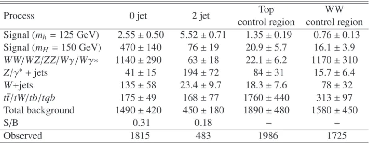
∆φ < π/2Table 1: The expected number of signal and background events for 13 fb
−1of integrated luminosity in the 0-jet channel and in the 2-jet channel after all selection cuts. The event yield of a potential signal is illustrated for a light Higgs boson with m
h =125 GeV and a heavy Higgs boson with m
H =150 GeV in a type-I 2HDM with tan
β =3 and
α = π/2. TheW+jets background is entirely determined from data [48]. The uncertainties quoted in the table are determined from the sum in quadrature of two sources: the total rate uncertainty, see Table 3, and the corresponding cross-section uncertainties. Since the W+jets background is derived from collision data the uncertainties of the data-driven estimation are used.
Process 0 jet 2 jet Top WW
control region control region Signal (m
h=125 GeV) 2.55
±0.50 5.52
±0.71 1.35
±0.19 0.76
±0.13 Signal (m
H=150 GeV) 470
±140 76
±19 20.9
±5.7 16.1
±3.9 WW/WZ/ZZ/Wγ/Wγ
∗1140
±290 63
±18 22.1
±6.2 1170
±310
Z/γ
∗+jets 41
±15 194
±72 84
±31 15.7
±6.4
W+jets 135
±58 23.4
±9.7 18.3
±7.6 78
±32
t t/tW/tb/tqb ¯ 175
±49 168
±77 1760
±440 313
±97 Total background 1490
±420 450
±180 1890
±480 1580
±450
S/B 0.31 0.18
− −Observed 1815 483 1986 1725
where
∆φminis the minimum separation
φangle between a lepton or a jet with p
T >25 GeV and E
Tmiss. The following pre-selection requirements for h/H
→WW
(∗)→eν µν candidates are imposed. They are the same as for the SM H
→WW
(∗)analysis [48]. Exactly two leptons of different flavour (electron or muon) and opposite charge are required. The lepton with the highest p
Tis called the leading lepton
ℓ1and must have p
T >25 GeV, while the second lepton
ℓ2fulfils p
T >15 GeV. The invariant mass of the two leptons m(ℓ
1ℓ2) is required to be larger than 10 GeV. The E
T,relmissis required to be at least 25 GeV.
This provides a strong suppression against multijet production via QCD processes and against the Z+jets background which originates predominantly from the Z
→τ+τ−decay channel.
After the preceding cuts the events are divided into two analysis channels: the 0-jet channel, in which exactly zero jets are required, and the 2-jet channel, which features exactly two jets. In the 0-jet channel there is a requirement on the absolute value of the difference in the azimuth angle
φof the two leptons,
|∆φ(ℓ1, ℓ2
)
| <2.4, and in addition m(ℓ
1ℓ2)
<75 GeV is required. These two cuts remove background in regions where only a small signal contribution is expected, such that the training of the NN can be focused on the more challenging phase space.
In the 2-jet channel events containing a b-tagged jet are rejected in order to suppress backgrounds involving top-quarks. The two jets are required to lie in opposite pseudorapidity hemispheres,
η(j
1)
× η(j
2)
<0, and m(ℓ
1ℓ2)
<80 GeV. Another cut is placed on the transverse mass m
Twhich is defined as
m
T= q(E
T(ℓ
1ℓ2)
+E
T(νν))
2−(
~p
T(ℓ
1ℓ2)
+E
~Tmiss)
2(2) where E
T(ℓ
1ℓ2)
=q
~
p
2T(ℓ
1ℓ2)
+m
2(ℓ
1ℓ2) and E
T(νν)
= q(E
missT)
2+m
2(ℓ
1ℓ2). It is required that m
T <180 GeV.
Table 1 shows the event yield of background and signal in the 0-jet channel and in the 2-jet channel
after all selection cuts. The signal was split into two rows to distinguish between the light Higgs bo-
son at m
h =125 GeV and the heavy Higgs boson at m
H=150 GeV in the 2HDM. The lowermost row
shows the observed numbers of events in the data. The diboson background (WW/WZ/ZZ/Wγ/Wγ
∗), the Z/γ
∗+jets background and the top-quark background (t¯ t/tW/tb/tqb) are estimated by using the theo- retical cross sections, detector acceptances from simulated events, and data-driven correction factors for identification and reconstruction efficiencies. In the subsequent statistical analysis the a-priori estimates are re-evaluated in the maximum-likelihood fit to the NN-discriminants and the event yield in a specifi- cally defined top-quark control region. In this fit the top-quark background is entirely free to float, while the diboson and Z/γ
∗+jets backgrounds are floating within the uncertainties of the a-priori estimate given in Table 1.
The W+jets background is estimated using a data-driven technique [48]. A control sample is defined by one lepton that satisfies all identification requirements as defined in the main analysis and one so- called anti-identified lepton that fails these criteria, but passes a looser selection. Except for the lepton identification the events in the W+jets control sample pass all other selections as required for the signal samples. To obtain an estimate of the number of W+jets in the signal sample, the efficiency
ǫfaketo misidentify an anti-identified lepton as a lepton has to be accounted for. A dijet data sample is used to determine
ǫfakeas a function of the p
Tof the anti-identified lepton. Residual contributions of leptons originating from W and Z decays are subtracted.
4 Signal and background discrimination
To separate 2HDM Higgs boson signal events from background in the WW
(∗)channel, several kinematic variables are combined to one discriminant in each of the two analysis channels by employing NNs.
The NeuroBayes [56] tool is used for preprocessing the input variables and for the training of the NNs.
A large number of input variables is studied, but only the highest-ranking variables are chosen for the training of the NNs. The ranking of the variables is automatically determined as part of the preprocessing step and is independent of the training procedure [57].
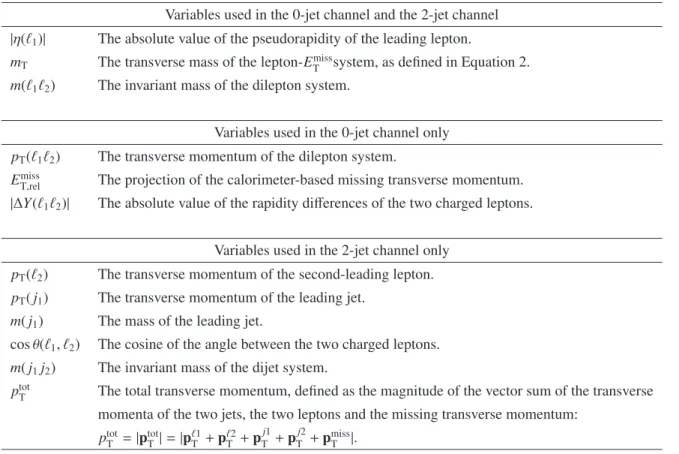
As a result of this optimisation procedure in the 0-jet channel, six kinematic variables are identified that serve as inputs to three NNs trained at three different Higgs boson mass points: m
H =150 GeV, 180 GeV, and 240 GeV. Dedicated studies showed that the NNs at these three mass points achieve the same sensitivity in terms of the expected exclusion contours in the cos
α–mHplane as a large number of NNs that are trained with a spacing of 5 GeV in m
H. The physical reason for this is the relatively low mass resolution in the H
→WW
(∗) →ℓ+νℓ−ν¯ channel of approximately 20 GeV. It was further studied that the addition of more variables to the NNs would lead only to an improvement well below 1% in the expected CLs values across the cos
α–mHplane. In the same way nine variables are selected in the 2-jet channel.
The selected variables are listed and explained in Table 2. The two most important input variables for the NN in the 0-jet channel trained at m
H=150 GeV are m(ℓ
1ℓ2) and m
T, while the two most important input variables for the NN in the 2-jet channel are m( j
1j
2) and m(ℓ
1ℓ2).
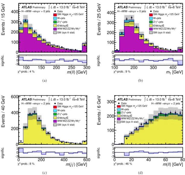
The modelling of the input variables is checked in two control regions that are enriched with the
dominating backgrounds: diboson production and t t ¯ production. The t t ¯ control region is obtained by
requiring at least one b-tagged jet. In the final statistical analysis, the t t-enriched control sample is ¯
included in order to determine the rate of t t ¯ events in situ. The diboson control region is defined by all
events passing the full event selection except the cut on m(ℓ
1ℓ2). Rather than m(ℓ
1ℓ2)
<75 GeV it is
required that m(ℓ
1ℓ2)
>80 GeV. To reduce the Z/γ
∗+jets background one additionally requires that
p
T(ℓ
1ℓ2)
>30 GeV. The two most important input variables of the two analysis channels are shown in
Fig. 2 in their respective control regions. Good modelling of the important diboson and t t ¯ backgrounds
is found.
Table 2: Input variables used for the NNs in the 0-jet and 2-jet channels. The definitions of the variables use the terms leading lepton and leading jet, defined as the lepton/jet with the highest p
T.
Variables used in the 0-jet channel and the 2-jet channel
|η(ℓ1)| The absolute value of the pseudorapidity of the leading lepton.
mT The transverse mass of the lepton-EmissT system, as defined in Equation 2.
m(ℓ1ℓ2) The invariant mass of the dilepton system.
Variables used in the 0-jet channel only pT(ℓ1ℓ2) The transverse momentum of the dilepton system.
EmissT,rel The projection of the calorimeter-based missing transverse momentum.
|∆Y(ℓ1ℓ2)| The absolute value of the rapidity differences of the two charged leptons.
Variables used in the 2-jet channel only pT(ℓ2) The transverse momentum of the second-leading lepton.
pT(j1) The transverse momentum of the leading jet.
m(j1) The mass of the leading jet.
cosθ(ℓ1, ℓ2) The cosine of the angle between the two charged leptons.
m(j1j2) The invariant mass of the dijet system.
ptotT The total transverse momentum, defined as the magnitude of the vector sum of the transverse momenta of the two jets, the two leptons and the missing transverse momentum:
ptotT =|ptotT |=|pℓ1T +pℓ2T +pTj1+pTj2+pmissT |.
) [GeV]
l l ( m
Events / 15 GeV
0 100 200 300 400
) [GeV]
l (l m
100 150 200 250 300
signific. -3
0 3
+ 0 jets ν µ ν
→e
→WW H
Preliminary
ATLAS ∫L dt = 13.0 fb-1 s=8 TeV Data
=125 GeV Higgs mh
SM W+jets
*+jets γ Z/
b /Wt/tq/t t t
γ* γ/W WW/WZ/ZZ/W
stat)
⊕ SM (sys
-prob.: 4 % χ2
(a)
[GeV]
mT
Events / 25 GeV
0 100 200 300 400
[GeV]
mT
100 200 300 400
signific. -3
0 3
+ 0 jets ν µ ν
→e
→WW H
Preliminary
ATLAS ∫L dt = 13.0 fb-1 s=8 TeV Data
=125 GeV Higgs mh
SM W+jets
*+jets γ Z/
b /Wt/tq/t t t
γ* γ/W WW/WZ/ZZ/W
stat)
⊕ SM (sys
-prob.: 9 % χ2
(b)
) [GeV]
j j ( m
Events / 40 GeV
0 200 400 600
) [GeV]
j j ( m
0 200 400 600
signific. -3
0 3
+ 2 jets ν µ ν
→e
→WW H
Preliminary
ATLAS ∫L dt = 13.0 fb-1 s=8 TeV Data
=125 GeV Higgs mh
SM W+jets
*+jets γ Z/
b /Wt/tq/t t t
γ* γ/W WW/WZ/ZZ/W
stat)
⊕ SM (sys
-prob.: 8 % χ2
(c)
) [GeV]
l l ( m
Events / 6 GeV
0 100 200 300
) [GeV]
l l ( m
0 20 40 60 80
signific. -3
0 3
+ 2 jets ν µ ν
→e
→WW H
Preliminary
ATLAS ∫L dt = 13.0 fb-1 s=8 TeV Data
=125 GeV Higgs mh
SM W+jets
*+jets γ Z/
b /Wt/tq/t t t
γ* γ/W WW/WZ/ZZ/W
stat)
⊕ SM (sys
-prob.: 46 % χ2
(d)
Figure 2: Distributions of the two highest-ranking input variables of the NN optimised for m
H=150 GeVin the diboson control region, (a) and (b), and in the t t ¯ control region, (c) and (d). The distributions
observed in collision data are compared to a model based on simulated events for which the contribution
of each process is normalised to the fitted event rate. The significance of deviations between the model
prediction and the observed data is shown in the lower histograms, following [58]. When computing the
significance only statistical uncertainties are taken into account.
NN output
0 0.2 0.4 0.6 0.8 1
Event fraction / 0.07
0 0.1 0.2 0.3
=180 GeV mH 2HDM
=125 GeV mh 2HDM Total background
NN @180GeV + 0 jets ν µ eν WW→ H→
Preliminary
ATLAS s = 8 TeV
(a)
NN output
0 0.2 0.4 0.6 0.8 1
Event fraction / 0.07
0 0.1 0.2 0.3
0.4 2HDM mH=180 GeV
=125 GeV mh 2HDM Total background
NN @180GeV + 2 jets ν µ eν WW→ H→
Preliminary
ATLAS s = 8 TeV
(b)
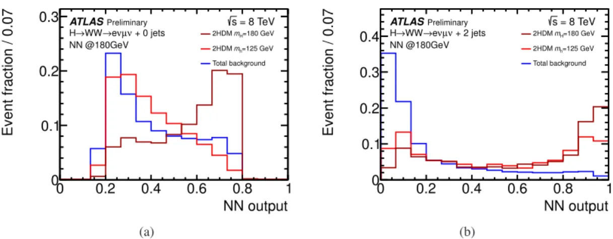
Figure 3: Normalised discriminant distributions (templates) obtained for the NN optimised at m
H =180 GeV for the 2HDM signal and background, (a) in the 0-jet channel and (b) in the 2-jet channel. The distributions are normalised to unit area.
Once a set of variables has been chosen based on the criteria outlined above, the analysis proceeds with the training of the NNs using a three-layer feed-forward architecture. Bayesian regularisation tech- niques are applied for the training process to damp statistical fluctuations in the training sample and to avoid overtraining. The ratio of signal to background events in the training is chosen to be 1:1, while the different background processes are weighted according to the number of expected events. The resulting distributions of the 2HDM signal and the total background normalised to unit area are shown in Fig. 3 for the NN optimised at m
H=180 GeV. The shape of the NN discriminant of the light Higgs boson h in a 2HDM is the same as the one of a pure SM Higgs boson. Only the predicted rate is changed.
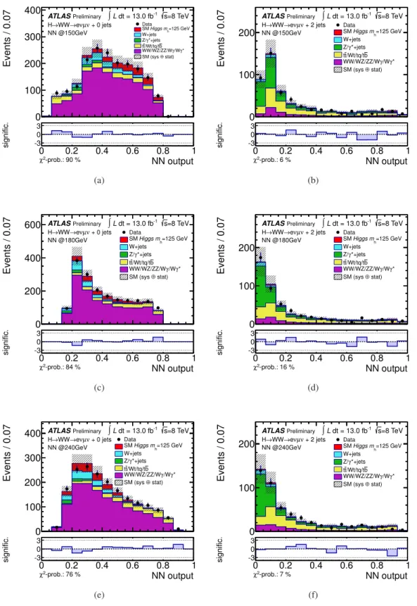
After the training is completed, the modelling of the NN-discriminant distributions is checked in the t t-enriched control region. One example of these cross-check distributions is shown in Fig. 4. The ¯ agreement between the model and the observed data is very good, and the next step of the analysis is the application of the NNs to the events in the signal samples. The corresponding distributions of the NN discriminants are shown in Fig. 5. The distributions observed in collision data are compared to a model
NN output
Events / 0.07
0 500 1000
NN output
0 0.2 0.4 0.6 0.8 1
signific. -3
0 3
NN @150GeV
+ 2 jets (CR) ν
µ ν
→e
→WW H
Preliminary
ATLAS ∫L dt = 13.0 fb-1 s=8 TeV
Data
=125 GeV Higgs mh
SM W+jets
*+jets γ Z/
b /Wt/tq/t t t
γ* γ/W WW/WZ/ZZ/W
stat)
⊕ SM (sys
-prob.: 14 % χ2
Figure 4: Discriminant distribution obtained with the NN optimised for m
H=150 GeV with the standard
training sample, but evaluated in the t t ¯ enriched control region in which at least one b-tagged jet is
required. The contribution of each process is normalised to the fitted event rate.
based on simulated events for which the contribution of each process is normalised to the fitted event rates including the SM Higgs boson. The fit is performed to the NN-discriminant distributions in 5(a) and 5(b), simultaneously. The fit results are applied to all other distributions in the signal region as well.
The fitted value of the SM Higgs boson event yield is compatible with that measured in the SM analysis in the WW
∗channel [48].
To cover the mass range of a potential heavy Higgs boson H from 135 GeV to 300 GeV the three NNs are applied in the following sub-ranges: the NN trained at m
H=150 GeV is evaluated at the mass points from 135 GeV to 160 GeV; the NN trained at m
H=180 GeV is applied in the range from 165 GeV to 200 GeV; and the NN trained at m
H =240 GeV is used at the mass points from 220 GeV to 300 GeV.
The evaluation of the background samples and the observed data remains the same for each NN, and only the distributions of the 2HDM Higgs boson samples vary from mass point to mass point. The statistical analysis of the resulting discriminant distributions is discussed in section 6.
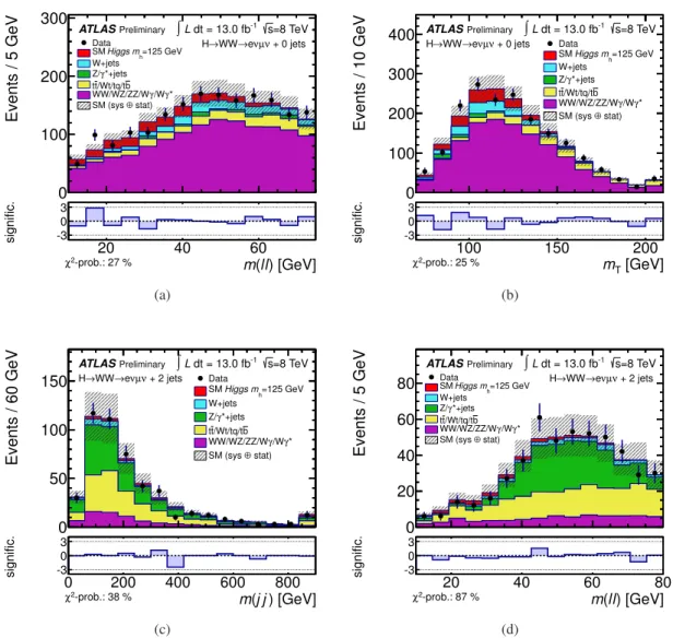
The distributions of the input variables are checked in the signal regions by comparing the data to
the distributions predicted by the model of simulated events normalised to the fitted event rates of the
different components, as described above. The distributions of the two most important variables in the
0-jet and 2-jet channels are shown in Fig. 6. A good agreement between data and the SM prediction is
found.
NN output
Events / 0.07
0 100 200 300 400
NN output
0 0.2 0.4 0.6 0.8 1
signific. -3
0 3
NN @150GeV + 0 jets ν µ ν
→e
→WW H
Preliminary
ATLAS ∫L dt = 13.0 fb-1 s=8 TeV
Data
=125 GeV Higgs mh SM W+jets
*+jets γ Z/
b /Wt/tq/t t t
γ* γ/W WW/WZ/ZZ/W
stat)
⊕ SM (sys
-prob.: 90 % χ2
(a)
NN output
Events / 0.07
0 100 200
NN output
0 0.2 0.4 0.6 0.8 1
signific. -3
0 3
NN @150GeV + 2 jets ν µ ν
→e
→WW H
Preliminary
ATLAS ∫L dt = 13.0 fb-1 s=8 TeV Data
=125 GeV Higgs mh
SM W+jets
*+jets γ Z/
b /Wt/tq/t t t
γ* γ/W WW/WZ/ZZ/W
stat)
⊕ SM (sys
-prob.: 6 % χ2
(b)
NN output
Events / 0.07
0 200 400 600
NN output
0 0.2 0.4 0.6 0.8 1
signific. -3
0 3
NN @180GeV + 0 jets ν µ ν
→e
→WW H
Preliminary
ATLAS ∫L dt = 13.0 fb-1 s=8 TeV Data
=125 GeV Higgs mh
SM W+jets
*+jets γ Z/
b /Wt/tq/t t t
γ* γ/W WW/WZ/ZZ/W
stat)
⊕ SM (sys
-prob.: 84 % χ2
(c)
NN output
Events / 0.07
0 100 200
NN output
0 0.2 0.4 0.6 0.8 1
signific. -3
0 3
NN @180GeV + 2 jets ν µ ν
→e
→WW H
Preliminary
ATLAS ∫L dt = 13.0 fb-1 s=8 TeV Data
=125 GeV Higgs mh
SM W+jets
*+jets γ Z/
b /Wt/tq/t t t
γ* γ/W WW/WZ/ZZ/W
stat)
⊕ SM (sys
-prob.: 16 % χ2
(d)
NN output
Events / 0.07
0 100 200 300 400
NN output
0 0.2 0.4 0.6 0.8 1
signific. -3
0 3
NN @240GeV + 0 jets ν µ ν
→e
→WW H
Preliminary
ATLAS ∫L dt = 13.0 fb-1 s=8 TeV Data
=125 GeV Higgs mh
SM W+jets
*+jets Z/γ
b /Wt/tq/t t t
γ* γ/W WW/WZ/ZZ/W
stat)
⊕ SM (sys
-prob.: 76 % χ2
(e)
NN output
Events / 0.07
0 100 200
NN output
0 0.2 0.4 0.6 0.8 1
signific. -3
0 3
NN @240GeV + 2 jets ν µ ν
→e
→WW H
Preliminary
ATLAS ∫L dt = 13.0 fb-1 s=8 TeV Data
=125 GeV Higgs mh
SM W+jets
*+jets γ Z/
b /Wt/tq/t t t
γ* γ/W WW/WZ/ZZ/W
stat) SM (sys ⊕
-prob.: 7 % χ2
(f)
Figure 5: Discriminant distributions obtained from the NNs for three different Higgs boson mass points in the 0-jet and the 2-jet channel. The distributions observed in collision data are compared to a model based on simulated events for which the contribution of each process is normalised to the fitted event rates including the SM Higgs boson. The fit is performed to the NN-discriminant distributions in (a) and (b) and the fit results are applied to the other distributions as well. The fitted value of the SM Higgs boson event yield is compatible with that measured in the SM analysis in the WW
∗channel [48]. The shape of the NN discriminant of the SM Higgs is the same as the one of the light Higgs boson h in a
2HDM with m
=125 GeV. 11
) [GeV]
l (l m
Events / 5 GeV
0 100 200 300
) [GeV]
l l ( m
20 40 60
signific. -3
0 3
+ 0 jets ν µ ν
→e
→WW H
Preliminary
ATLAS ∫L dt = 13.0 fb-1 s=8 TeV Data
=125 GeV Higgs mh
SM W+jets
*+jets γ Z/
b /Wt/tq/t t t
γ* γ/W WW/WZ/ZZ/W
stat)
⊕ SM (sys
-prob.: 27 % χ2
(a)
[GeV]
mT
Events / 10 GeV
0 100 200 300 400
[GeV]
mT
100 150 200
signific. -3
0 3
+ 0 jets ν µ ν
→e
→WW H
Preliminary
ATLAS ∫L dt = 13.0 fb-1 s=8 TeV Data
=125 GeV Higgs mh
SM W+jets
*+jets γ Z/
b /Wt/tq/t t t
γ* γ/W WW/WZ/ZZ/W
stat)
⊕ SM (sys
-prob.: 25 % χ2
(b)
) [GeV]
j j ( m
Events / 60 GeV
0 50 100 150
) [GeV]
j j ( m
0 200 400 600 800
signific. -3
0 3
+ 2 jets ν µ eν WW→ H→
Preliminary
ATLAS ∫L dt = 13.0 fb-1 s=8 TeV Data
=125 GeV Higgs mh
SM W+jets
*+jets γ Z/
b /Wt/tq/t t t
γ* γ/W WW/WZ/ZZ/W
stat)
⊕ SM (sys
-prob.: 38 % χ2
(c)
) [GeV]
l l ( m
Events / 5 GeV
0 20 40 60 80
) [GeV]
l l ( m
20 40 60 80
signific. -3
0 3
+ 2 jets ν µ eν WW→ H→
Preliminary
ATLAS ∫L dt = 13.0 fb-1 s=8 TeV Data
=125 GeV Higgs mh
SM W+jets
*+jets γ Z/
b /Wt/tq/t t
t γ/Wγ*
WW/WZ/ZZ/W stat)
⊕ SM (sys
-prob.: 87 % χ2
(d)
Figure 6: Distributions of the two highest-ranking input variables of the NN optimised for m
H=150 GeVin the signal region of the 0-jet channel, (a) and (b), and in the signal region of the 2-jet channel, (c) and
(d). The distributions observed in collision data are compared to a model based on simulated events for
which the contribution of each process is normalised to the fitted event rates including the SM Higgs
boson. The fit is performed to the NN-discriminant distributions in Figs. 5(a) and (b). The fitted value
of the SM Higgs boson event yield is very well compatible with that measured in the H
→WW
∗SM analysis [48]. The significance of deviations between the model prediction and the observed data
is shown in the lower histograms, following [58]. When computing the significance only statistical
uncertainties are taken into account.
5 Systematic uncertainties
Systematic uncertainties in the normalisation of the different backgrounds, on the signal acceptance, and on the shape of the NN-discriminant distributions for signal and background processes reduce the sensitivity of the search for Higgs boson production. Systematic uncertainties arise due to the limited understanding of the residual differences between data and Monte Carlo simulations for the reconstruc- tion and energy calibration of jets, electrons, and muons. Other sources of systematic uncertainties are due to the modelling of physics processes in simulations. All uncertainties are fully propagated through the entire analysis. The following categories of systematic uncertainties are considered:
Jet modelling
The main source of uncertainty on the modelling of jets comes from the jet energy scale (JES) [59]. For the jet definition applied in this analysis, the JES uncertainty varies from 2% to 14% as a function of p
Tand
η. An additional contribution to the JES uncertainty is caused by pile-up effects andranges from less than 1% to 4% as a function of jet p
Tand
η. Forb-quark induced jets an additional JES uncertainty of 0.8% to 2.5%, depending on the jet p
T, is added in quadrature to the JES uncertainty.
Scale factors, determined from collision data [60], are applied to correct the b-tagging performance in simulated events to match the data. The uncertainties in the scale factors vary from 10% to 20% for b-jets.
For light-quark jets, the mis-tagging uncertainty ranges from 20% to 50% as a function of jet p
Tand
η.Uncertainties in the modelling of the jet energy resolution (JER) also contribute and are estimated from collision data. Additional uncertainties arise from the modelling of jets with p
T <20 GeV as well as from soft energy deposits in the calorimeter that are not associated with reconstructed physics objects.
Other minor uncertainties are assigned to the reconstruction of E
missTand to account for the impact of pile-up collisions on E
missT.
Lepton modelling
Uncertainties in the electron and muon reconstruction, identification, and trigger efficiencies are estimated using tag-and-probe methods on samples enriched with Z
→ℓℓ,J/ψ
→ℓℓ,or W
± →ℓν(ℓ
=e, µ) events. Other components include the electron and muon energy scale.
Luminosity
The uncertainty on the integrated luminosity is 3.6%. It is derived, following the same methodology as that detailed in Ref. [61], from a preliminary calibration of the luminosity scale derived from beam-separation scans performed in April 2012.
PDFs
The systematic uncertainties related to the parton distribution functions are taken into account for all samples using simulated events. The events are reweighted according to each of the PDF uncertainty eigenvectors. The uncertainties are calculated using the formula given in Equation 43 of Ref. [62]. The envelope is calculated, following the PDF4LHC recommendation, of the estimated uncertainties for the CT10 PDF set, the MSTW2008nlo [63] PDF set, and the NNPDF2.0 [64] set as final PDF uncertainty.
Generator and parton shower
Uncertainties in the modelling of the event kinematics with Monte Carlo generators are taken into account for the top-quark background and the diboson background. The uncertainty due to the choice of POWHEG as generator for the diboson background is estimated by comparing the event rate and the shape of the NN discriminants to the ones obtained with MC@NLO.
The generator uncertainty on the t¯ t background is estimated by comparing MC@NLO and ALPGEN.
In addition, uncertainties are assigned to the modelling of the parton showers and hadronisation by interchanging the modelling between PYTHIA and HERWIG.
Pile-up
The uncertainty on the modelling of pile-up events is determined by varying the average num-
ber of collisions per bunch crossing in simulated events.
MC statistics
The impact of using simulation samples of limited size is also taken into account. This is done by generating pseudo-experiments, where the probability density of the NN discriminants (tem- plates) is varied within their statistical uncertainty.
Background rates
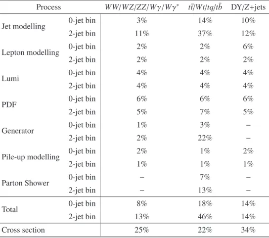
The rate of top-quark background is normalised using the event yield in a con- trol region as one component in the maximum-likelihood fit. However, when generating the pseudo- experiments for the statistical analysis the theoretical cross-section uncertainty of 22% is taken into account. The W+jets background arises from a jet being misidentified as a lepton. The uncertainty on understanding the misidentification rate and the resulting W+jets event rate is 43% in the 0-jet channel and 41% in the 2-jet channel (see section 3). The diboson and Z+jets backgrounds are normalised ac- cording to the cross sections predicted by theoretical computations and the corresponding uncertainties are quoted in Table 3.
Signal cross-section
The relative uncertainty on the signal cross sections (gluon fusion, VBF and W H/ZH) is determined following Ref. [65, 66]. The relative cross-section uncertainty of these processes is assumed to be 25% for gluon fusion in the 0-jet channel and 30% in the 2-jet channel, while the uncertainty on the combined VBF/W H/ZH category is 10%. These uncertainties also account for un- certainties in the modelling of the underlying event. The cross-section uncertainties in the gluon-fusion process are treated uncorrelated between the 0-jet channel and the 2-jet channel, since they arise from different sources.
The rate and cross-section uncertainties of the background processes that are modelled based on
simulated events are summarised in Table 3.
Table 3: Relative systematic rate uncertainties for background processes in the 0-jet channel and the 2-jet channel. The uncertainties are rounded to full per cent, but all uncertainties that are smaller than 1% are rounded up. As described in the text above, the exact value of the luminosity uncertainty is 3.6% for each process. DY stands for Drell-Yan processes and the single top-quark processes are denoted Wt/tq/t b. ¯
Process WW/WZ/ZZ/Wγ/Wγ
∗t t/Wt/tq/t ¯ b ¯ DY/Z+jets
Jet modelling 0-jet bin 3% 14% 10%
2-jet bin 11% 37% 12%
Lepton modelling 0-jet bin 2% 2% 6%
2-jet bin 2% 2% 2%
Lumi 0-jet bin 4% 4% 4%
2-jet bin 4% 4% 4%
PDF 0-jet bin 6% 6% 6%
2-jet bin 5% 7% 5%
Generator 0-jet bin 1% 3%
−2-jet bin 2% 22%
−Pile-up modelling 0-jet bin 2% 1% 2%
2-jet bin 1% 1% 1%
Parton Shower 0-jet bin
−7%
−2-jet bin
−13%
−Total 0-jet bin 8% 18% 14%
2-jet bin 13% 46% 14%
Cross section 25% 22% 34%
6 Hypothesis tests
To estimate the signal content of the selected samples, a maximum-likelihood fit is performed to the NN output distributions and to the event yield in the t t ¯ control region. Including all bins of the NN output distributions in the fit has the advantage of making maximal use of all signal events remaining after the event selection, and, in addition, allows for constraining the background rates from the data. The likelihood fit is performed simultaneously in both signal channels, that is the 0-jet channel and the 2-jet channel, and in the t t ¯ control region where only the event yield is considered, since it is very pure and discrimination between different processes is not needed. The sensitivity to the background rates is given by the background dominated region of the NN output distribution, that is the region close to zero, and the event yield in the t t ¯ control region.
The likelihood function is given by the product of Poisson probability terms for the individual his- togram bins. The background rates, except for the t¯ t background, are constrained by Gaussian priors that are added multiplicatively to the likelihood function. Within the likelihood function the predicted signal and background rates are multiplied by scale factors
βsfor the signal and
βbjfor the backgrounds, respectively; with the index j running over all background processes.
6.1 The q-value test statistic
The compatibility of the observed data with the different signal hypotheses, which depend on the parame- ters of the 2HDM, and the background-only hypothesis is evaluated by performing frequentist hypotheses tests based on pseudo-experiments. Two hypotheses are compared. The null hypothesis H
0assumes, that there is no Higgs boson at all. The signal hypothesis H
1assumes a Higgs boson signal as predicted by a specific 2HDM, depending on the values of cos
α, tanβ, andm
H. The Higgs-like boson observed at 125 GeV is part of the signal hypothesis, assuming that it is the h of a 2HDM. The signal strength of the h boson used in the statistical test is the one predicted by the 2HDM under consideration. In addition, the signal hypothesis includes the contribution of the H boson. For both scenarios ensemble tests, that is large sets of pseudo-experiments, are performed. To distinguish between the two hypotheses the so- called q value is used as a test statistic. It is defined as minus two times the difference of the logarithm of the maximum of the likelihood function evaluated when fixing the signal cross sections to their predicted values in 2HDM (β
sj =1) and found by setting the signal cross sections to zero (β
sj =0). The background scale factors
βbjare left free to float in both cases within their uncertainties. The two fits yield the two maxima
L(β
s=1,
βˆˆ
b,1j) and
L(β
s=0,
βˆˆ
b,0j), respectively, and the q value is then defined as
q
≡ −2 ln
L
βs=
1,
βˆˆ
b,1j /L
βs=
0,
βˆˆ
b,0j.