Search for a high-mass Higgs boson in the H→WW→`ν`ν decay channel with the ATLAS detector using 21 fb

ATLAS-CONF-2013-067 18July2013

ATLAS NOTE

ATLAS-CONF-2013-067

July 15, 2013

Search for a high-mass Higgs boson in the H→WW→`ν`ν decay channel with the ATLAS detector using 21 fb

of proton-proton collision data

The ATLAS Collaboration

Abstract

A search by the ATLAS experiment at the Large Hadron Collider for a Higgs boson in the H→WW →`ν`ν channel in the range 260 GeV < m

< 1 TeV is presented. The analysis uses proton-proton collision data at a centre-of-mass energy of 8 TeV, corresponding to an integrated luminosity of 20.7 fb

. A Higgs boson with Standard Model-like couplings is excluded at 95% confidence level in the mass range 260 GeV < m

< 642 GeV.

c

Copyright 2013 CERN for the benefit of the ATLAS Collaboration.

Reproduction of this article or parts of it is allowed as specified in the CC-BY-3.0 license.

1 Introduction

The Standard Model (SM) [1–3] of electroweak interactions has been tested to very high precision over the past decades. It predicts the existence of a scalar field which is responsible for spontaneous symmetry breaking in the electroweak theory [4–6]. This field is responsible for giving mass to SM particles. In addition, it acquires a non-vanishing vacuum expectation value and is manifested by a massive resonance, the SM Higgs boson, the mass of which is not predicted.

The boson discovered in 2012 by the ATLAS [7] and CMS [8] collaborations at the LHC is possibly the SM Higgs boson. Measurements of its properties show consistency with predictions of the SM [9–11]. However, since these measurements do not conclusively establish it as the SM Higgs boson, it is important to continue the Higgs boson search over the full mass range explorable at the LHC. Furthermore, there are extensions of the SM which are compatible with the current results and which predict the existence of additional neutral Higgs-like resonances in the high-mass regime.

Examples include Two Higgs Doublet Models (2HDMs) [12–14] and generic models in which the SM Higgs boson mixes with a heavy electroweak singlet [15–20] in order to complete the unitarisation of WW scattering at high energies. In particular, if measured values of signal strengths and universal couplings of the resonance near 125 GeV [10] are interpreted in these Beyond the SM (BSM) models, a second heavier Higgs-like boson with a narrow width is favoured in some regions of the parameter space.

The ATLAS Collaboration has previously reported the results of a search in the H→WW →`ν`ν channel (with ` = e, µ) using 4.7 fb

of proton-proton ( pp) collision data collected at √

s = 7 TeV [21]

at the LHC. In this search, a SM-like Higgs boson in the mass range 133 GeV < m

< 261 GeV was excluded at 95% confidence level (CL). A search in this channel for a heavy Higgs boson in 2HDM models using 13 fb

of data at √

s = 8 TeV was reported in Ref. [22].

This note presents a heavy Higgs boson search by the ATLAS Collaboration in the H→WW →`ν`ν (` = e, µ) channel in the mass range 260 GeV < m

< 1 TeV using 20.7 fb

of pp collision data at √

s = 8 TeV. Only the different lepton-flavour final state (eνµν) is used. Decays via τ leptons, such as H→WW →`ντν (with τ → `νν) are included. The contribution from the observed resonance at m

∼ 125 GeV is treated as a background. The analysis in performed using two largely di ff erent assumptions on the width of the Higgs boson or of a scalar resonance. In addition to the Standard Model width (Higgs boson) a narrow width is assumed.

Section 2 of this note describes the data sample and physics object reconstruction. Section 3 summarises the simulation of physics processes. The event selection is detailed in Section 4, while Section 5 presents background estimation techniques. Systematic uncertainties affecting the analysis are discussed in Section 6. Results are presented in Section 7, and the conclusions of the study are summarised in Section 8.

2 Data sample and object reconstruction

The data sample used for this analysis was collected using the ATLAS detector, a multi-purpose par- ticle physics detector with a forward-backward symmetric cylindrical geometry and near-4π coverage in solid angle [23]. Because of the high LHC peak luminosity and a bunch separation of 50 ns, the number of proton–proton interactions occurring in the same bunch crossing is large (on average 20.7).

This is referred to as event “pile-up”

and requires the use of dedicated algorithms and corrections to mitigate its impact on the reconstruction of, e.g. leptons and jets.

1Multipleppcollisions occuring in the same (nearby) bunch crossing are denoted as in-time (out-of-time) pile-up.

Events in the data sample are triggered requiring at least one isolated muon or electron with trans- verse momentum p

> 24 GeV. The lepton trigger e ffi ciencies are measured using Z boson candidates as a function of p

and pseudorapidity

η. The trigger e ffi ciencies for the leptons used in this analysis are approximately 70% for muons with | η | < 1.05, 90% for muons in the range 1.05 < | η | < 2.4, and

≥ 95% for electrons in the range | η | < 2.4.

Events are required to have a primary vertex consistent with the beam spot position, with at least three associated tracks with p

> 0.4 GeV. Data quality criteria are applied to events in order to suppress non-collision backgrounds such as cosmic-ray muons, beam-related backgrounds or noise in the calorimeters.

Electron candidates are required to have a well-reconstructed track in the inner detector pointing to a cluster of cells with energy depositions in the electromagnetic calorimeter. A set of tight identi- fication criteria including both tracking and calorimeter shower shape information is used. The fine lateral and longitudinal segmentation of the calorimeter and the transition radiation detection capa- bility of the ATLAS detector allow for robust electron reconstruction and identification [24] in the high pile-up environment. In this analysis, electrons are required to be in the range | η | < 2.47 ex- cluding 1.37 < | η | < 1.52 which corresponds to the transition region between the barrel and endcap calorimeters.

Muon candidates are identified by matching tracks reconstructed in the inner detector with tracks reconstructed in the muon spectrometer [25]. Muons are required to be in the range | η | < 2.5.

Jets are reconstructed from topological clusters of calorimeter cells [26] using the anti-k

algo- rithm with distance parameter R = 0.4 [27]. The jet energy dependence on pile-up is mitigated by applying two data-derived corrections: one based on the product of the event p

density and the jet area [28], and another that depends on the number of reconstructed primary vertices and the mean number of expected interactions. After these corrections, an energy- and η-dependent calibration is applied to all jets. Finally, a residual correction from in situ measurements is applied to refine the jet calibration [29]. The analysis requires the jets to have p

> 25 GeV if | η | < 2.4 and p

> 30 GeV for 2.4 < | η | < 4.5. The increased threshold in the forward region reduces the contribution from jet candidates produced by pile-up. To reduce the pile-up contribution further, jets within the inner de- tector acceptance (|η| < 2.47) are required to have more than 50% of the sum of the scalar p

of their associated tracks coming from tracks associated to the primary vertex.

Jets originating from b-quarks are identified using a multi-variate b-tagging algorithm [30] which combines impact parameter information of tracks and the reconstruction of charm and bottom hadron decays. This analysis uses an algorithm which has an e ffi ciencyof 85% for b-jets and a mis-tag rate for light-flavour jets of 11% in simulated t¯ t events [30].

The missing transverse momentum, E

[31], is the magnitude of the negative vector sum of the transverse momenta p ~

of the muons, electrons, photons, jets and clusters of calorimeter cells with | η | < 4.9 not associated with these objects. Di ff erent selection criteria based on E

are used depending on the jet multiplicity.

2The ATLAS experiment uses a right-handed coordinate system with its origin at the nominal interaction point (IP) in the centre of the detector and thez-axis along the beam line. Thex-axis points from the IP to the centre of the LHC ring, and they-axis points upwards. Cylindrical coordinates (r, φ) are used in the transverse plane,φbeing the azimuthal angle around the beam line. The pseudorapidity is defined in terms of the polar angleθasη=−ln tan(θ/2).

3 Simulated physics samples

Signal contributions considered in this analysis include the gluon-gluon fusion production process (gg → H, denoted as ggF) and the vector-boson fusion production process (q

q

→q

q

H, denoted as VBF). Contributions from Higgs-strahlung and t¯ tH production mechanisms are not considered owing to their very small cross sections at high Higgs boson masses. The H→WW→`ν`ν (with ` = e, µ) final state is considered, including the small contribution from leptonic W → τν → `νν ν decays. The branching fractions for the decays as a function of m

have been calculated using P4 [32,33]

with H  used to calculate the total width [34].

The ggF signal cross section includes corrections up to next-to-next-to-leading order (NNLO) in QCD [35–40]. Next-to-leading order (NLO) electroweak (EW) corrections are also applied [41,42], as well as QCD soft-gluon resummations up to next-to-next-to-leading logarithmic order (NNLL) [43].

These calculations are detailed in Refs. [44–46] and assume factorisation between the QCD and EW corrections. The VBF signal cross section is computed with approximate NNLO QCD corrections [47]

and full NLO QCD and EW corrections [48–50].

The final results are interpreted in the SM scenario as well as in a scenario which uses a narrow- width approximation (NWA). Consequently, two di ff erent sets of simulated signal samples have been used: SM samples in the mass range 260 GeV ≤ m

≤ 1 TeV and NWA samples in the mass range 300 GeV ≤ m

≤ 1 TeV. In the SM scenario, the lineshape of the WW invariant mass distribution of the signal samples is well-described by a Breit-Wigner distribution with a running width [44] up to m

∼ 400 GeV. Therefore, for m

< 400 GeV, ggF [51] and VBF P [52]+P8 [53] samples generated with a running width Breit-Wigner propagator are used. For m

≥ 400 GeV, the Breit- Wigner description is no longer valid and the complex-pole scheme (CPS) [54–56] instead provides a more accurate description. The CPS propagator is therefore used to describe the lineshape of both ggF and VBF Higgs boson signal samples for m

≥ 400 GeV. The corresponding samples are generated with P + P  8. The calculations using the Breit-Wigner and the CPS are in good agreement in the mass range below ∼ 400 GeV.

For a Higgs boson with a large width, the production cross section as well as kinematic variables are a ff ected by the interference between signal and non-resonant WW background production. This effect is small for a SM Higgs boson with m

< 400 GeV. The impact of the interference increases with increasing Higgs boson width and its inclusion is important for m

≥ 400 GeV. Calculations of the interference e ff ect are available only at leading order accuracy, and it is not included in the ggF and VBF P+P8 signal samples used in the analysis. Consequently, the signal samples are weighted to take the effect of interference into account. The weights are computed using MCFM v6.2 [57] and the REPOLO tool provided by the authors of VBFNLO [58] in the ggF and in the VBF case, respectively. Theoretical uncertainties on the interference weighting due to missing higher- order terms are included in the total uncertainty [20], in addition to EW corrections. It has been demonstrated that the weighting is valid for all kinematic variables used in this analysis. The full weighting procedure, including the treatment of the associated uncertainties, is detailed in Ref. [20].

For the interpretation of a heavy SM-like Higgs boson with a narrow width, P +P  8 NWA signal samples with a fixed 1 GeV wide Breit-Wigner lineshape have been used. Because of the narrow width, the effect of interference between signal and continuum background is negligible over the full mass range [59, 60], so that no interference weighting is applied to these samples.

The Monte Carlo (MC) generators [52–54,61–68] used to model signal and background processes

are listed in Table 1. In this table, all W and Z boson decays into leptons (e, µ, τ) are included in

the corresponding product of the cross section (σ) and the branching ratio (B). Further details on the

cross section calculations can be found in Ref. [69].

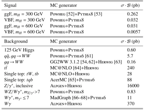
Table 1: Monte Carlo generators used to model the signal and background processes. All leptonic decay branching ratios (e, µ, τ) of the W and Z bosons are included in the product of cross section (σ) and branching ratio (B), except for top-quark production, for which the inclusive cross section is quoted. For the signal samples, σ · B (H→WW→`ν`ν with ` = e, µ, τ) are given; representative values are shown for m

= 300 GeV and 600 GeV.

Signal MC generator σ · B (pb)

ggF, m

= 300 GeV P [52]+P8 [53] 0.262

VBF, m

= 300 GeV P + P  8 0.032

ggF, m

= 600 GeV P + P  8 0.031

VBF, m

= 600 GeV P+P8 0.0057

Background MC generator σ · B (pb)

125 GeV Higgs P + P  8 0.60

q q, ¯ gq →WW P+P6 [61] 5.7

gg → WW GG2WW 3.1.2 [54, 62]+H  [63] 0.16

t¯ t MC@NLO [64] + H  240

Single top: tW , tb MC@NLO+H 28

Single top: tqb AcerMC [65]+P  6 88

Z/γ

, inclusive A + H  16000

WZ/Wγ

, m

>7 P+P8 0.83 Wγ

, m

≤ 7 MadGraph [66–68]+P  6 11

Wγ A + H  370

For most processes, separate programs are used to generate the hard scattering and to model the parton showering (PS), hadronisation and underlying event (UE). P8 or P6 are used for the latter three steps for the signal and for some of the background processes. When H  is used for the hadronisation and PS, the UE is modelled using J  [70]. The W + jets, Z/γ

+ jets and Wγ processes are described using the A+H generator with the MLM matching scheme described in Ref. [71].

The parton distribution function (PDF) set from CT10 [72] is used for the P  and MC@NLO samples, while CTEQ6L1 [73] is used for the A, MadGraph and P6/P8 samples.

Acceptances and e ffi ciencies are obtained from a full simulation [74] of the ATLAS detector using G  4 [75]. In two cases (q q ¯ → WW and single top processes), fast simulation is used to increase the number of MC events. The simulation incorporates a model of the event pile-up conditions in the data, including both in-time and out-of-time pile-up.

4 Event selection

The high pile-up environment of the 2012 data-taking degrades the resolution of E

, which results in a large Drell-Yan (Z/γ

→ ``) background in the same lepton flavour final states (eνeν and µνµν).

Since most of the sensitivity of the analysis comes from the different-flavour final state (eνµν), only

this one is used. Therefore, the final state topology consists of an oppositely charged pair of an

electron and a muon, and large E

. The dominant background contributions are from continuum

WW, t¯ t and Wt production, all of which produce two W bosons as the signal. Drell-Yan events, mainly from the Z/γ

→ ττ → eννµνν decay, can pass the signal selection when they are reconstructed with significant E

, while W + jets production with a jet mis-reconstructed as a lepton can also lead to the same final state. Diboson processes such as Wγ

and WZ

make very small contributions to this high-mass search; these are collectively referred to as VV processes in the following. The m

= 125 GeV boson is treated as a background; its production rate is a parameter in the likelihood fit.

Both signal and background compositions depend strongly on the final state jet multiplicity (N

).

For N

≤ 1, the signal is predominantly from the ggF process and WW events dominate the back- ground. For N

≥ 2, the signal originates mostly from the VBF process and t¯ t events dominate the background. The analysis is consequently divided into N

= 0, 1 and ≥ 2 categories.

Events are required to have one electron and one muon, oppositely charged, one of which must match the object that triggered the event. Both leptons are required to have p

> 40 GeV, and stringent track- and calorimeter-based isolation criteria are applied to reject background from W +jets and multi- jet production. Background from low-mass γ

→ττ → eννµνν makes a significant contribution and is rejected by requiring the dilepton invariant mass m

> 10 GeV. These selections form the event pre- selection.

Multi-jet and Drell-Yan backgrounds are further suppressed by requiring large E

. For N

≤ 1, a requirement is used on E

= E

· sin | ∆ φ

|, where ∆ φ

is the smallest azimuthal angle between the E

vector and any jet or high- p

electron or muon in the event. If | ∆ φ

| > π/2, then E

= E

is taken. Figure 1a shows the E

distribution after the pre-selection requirements, summed over all jet multiplicities. E

> 25 GeV is required for N

≤ 1. In the N

≥ 2 final state, however, the large number of jets reduces the signal efficiency of the E

criterion, such that a requirement on E

is used, namely, E

> 20 GeV. The jet multiplicity distribution following the pre-selection and the E

selections is shown in Fig. 1b.

In the N

= 0 final state, the transverse momentum of the dilepton system is required to be large, p

> 30 GeV in order to reject residual Drell-Yan events. To remove events that may have been badly reconstructed, the azimuthal separation between the p

and E

vectors is required to sat- isfy ∆ φ

T

> π/2.

In the N

= 1 final state, the top-quark background is suppressed by vetoing events with a b- tagged jet. The Z/γ

→ττ background is suppressed by using an invariant mass m

computed under the assumption that the neutrinos are collinear with the leptons in the τ decay [76] and that they are the only source of E

. Events compatible with a Z → ττ decay are rejected by requiring

| m

− m

| ≥ 25 GeV.

The N

≥ 2 final state has been optimised for the selection of the VBF production process.

The two leading jets (“tagging jets”), are required to have a large separation in rapidity y, namely

| ∆ y

| > 2.8, and a high invariant mass, m

> 500 GeV. To reduce the contribution from ggF pro- duction, events with any jet with p

> 20 GeV in the rapidity gap between the two tagging jets are rejected. Both leptons are required to be in this rapidity gap. The same b-jet and Z → ττ vetoes as in the N

= 1 final state are applied. The t¯ t background is further reduced by requiring a small total transverse momentum, p

< 45 GeV, where p

= p

+ p

+ E

, with p

being the vector sum of the transverse momenta of the tagging jets.

For all jet multiplicities, topological selections that exploit the kinematic features of the WW →`ν`ν

decay of a high-mass Higgs boson are employed. A dilepton invariant mass selection of m

> 50 GeV

is required: this criterion is e ffi cient in rejecting the contamination of the m

= 125 GeV state, the

decay of which produces leptons with low values of m

. The pseudorapidity di ff erence between the

leptons, ∆ η

, is required to be less than 1. This criterion reduces backgrounds due to WW and top-

[GeV]

T,rel

Emiss

0 50 100 150 200 250

Events / 5 GeV

10-2

10-1

1 10 102

103

104

105

106

107

Data stat)

⊕ SM (sys

t t WW Single Top Z+jets

γ WZ/ZZ/W W+jets H [125 GeV]

H [300 GeV]

H [600 GeV]

H [900 GeV]

ATLAS Preliminary

Ldt = 20.7 fb-1

∫

= 8 TeV s

ν µ ν

→ e

→WW H

(a)

Njets

0 2 4 6 8 10

Events

0 1000 2000 3000 4000 5000 6000

7000 Data

stat)

⊕ SM (sys

t t WW Single Top Z+jets

γ WZ/ZZ/W W+jets H [125 GeV]

H [300 GeV]

×10) H [600 GeV] (

×10) H [900 GeV] (

ATLAS Preliminary

Ldt = 20.7 fb-1

∫

= 8 TeV s

ν µ ν

→ e

→WW H

(b)

Figure 1: (a) Missing transverse momentum distribution for all events, summed over jet multiplicities, after the pre-selection. (b) Jet multiplicity for events after the pre-selection and the requirements on E

. The shaded area represents the uncertainty on the signal and background yields from statistical, experimental and theoretical sources. Signal expectations for m

= 300 GeV, 600 GeV and 900 GeV are shown, with ggF and VBF contributions added. In (a), the rightmost bin includes the events in overflow. In (b), the m

= 600 GeV and 900 GeV signals have been scaled by a factor of 10 to enhance visibility. The m

= 125 GeV state, treated as a background, is also shown, though it is too small to be visible after the pre-selection.

quark production in all jet multiplicities, and in addition can be used to define a WW control region in the N

≤ 1 final states, as discussed in Section 5. The event selection criteria are summarised in Table 2.

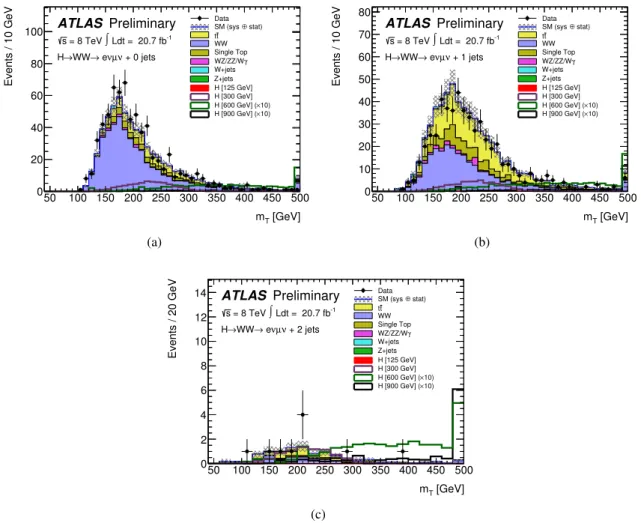
The discriminating variable used in the final likelihood fit to data is the transverse mass m

, de- fined as m

= ((E

+ E

)

− | p

+ E

|

)

with E

= (| p

|

+ m

)

. Figure 2 shows the m

distributions of the expected signals and backgrounds in the di ff erent N

final states.

5 Background estimation

The dominant backgrounds are top-quark and WW production, followed by W /Z + jets and VV pro-

cesses. The W +jets background is estimated using a data-driven method. The small Z +jets and VV

backgrounds are normalised using simulation. The top-quark and WW backgrounds are normalised

to data in control regions (CRs) defined by criteria similar to those used for the signal region, but

with some requirements reversed or modified to obtain signal-depleted samples enriched in particular

backgrounds. To estimate the event yield in a CR, first the contributions from backgrounds other than

the intended one are subtracted from the initial number of events. These contributions are determined

using either simulation or data-driven methods. For example, to determine the event yield in the WW

CR in the N

= 0 final state, the top-quark background, estimated using the method summarised be-

low, is subtracted from the initial event yield. Similarly, W /Z + jets and VV contributions are subtracted

to obtain the WW event yield in this CR, defined below. The yield is then extrapolated to the signal

region using simulation.

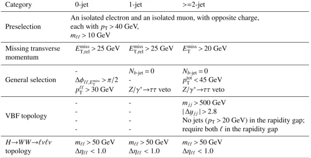
Table 2: Event selection used in the analysis. The preselection applies to all final states. In the N

≥ 2 final state, the rapidity gap is the y range spanned by the two leading jets.

Category 0-jet 1-jet >=2-jet

Preselection

An isolated electron and an isolated muon, with opposite charge, each withpT>40 GeV,

m``>10 GeV Missing transverse

momentum

E^miss_T,rel>25 GeV E^miss_T,rel>25 GeV E^miss_T >20 GeV

General selection

- Nb-jet=0 Nb-jet=0

∆φ_``,Emiss

T > π/2 - p^tot_T <45 GeV

p^``_T >30 GeV Z/γ^∗→ττveto Z/γ^∗→ττveto

VBF topology

- - mj j>500 GeV

- - |∆y_{j j}|>2.8

- - No jets (p_T>20 GeV) in the rapidity gap;

- - require both`in the rapidity gap

H→WW→`ν`ν topology

m``>50 GeV m``>50 GeV m``>50 GeV

∆η_{``</sub><1.0 ∆η<sub>``}<1.0 ∆η_``<1.0

5.1 t t ¯ and single top

The top-quark background in the N

= 0 final state is estimated using the procedure detailed in Ref. [7]. The number of events in data with any number of reconstructed jets passing the E

re- quirement (a sample dominated by top-quark background), is multiplied by the fraction of top-quark events with no reconstructed jets, obtained from simulation. This estimate is corrected using a CR defined by requiring at least one b-tagged jet after the E

selection.

The top-quark background in the N

≥ 1 channels is normalised to the data in a CR defined by requiring exactly one b-tagged jet and all other signal selections in the relevant final state except for the requirements on m

and ∆ η

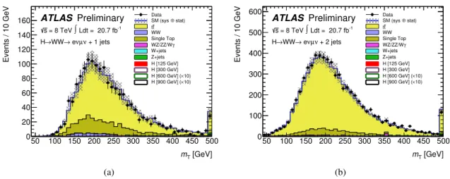
. Figure 3 shows the m

distribution for signals and backgrounds in the N

= 1 and N

≥ 2 top CRs. Good agreement between data and the prediction is obtained in both final states.

5.2 WW

In the N

≤ 1 final states, the WW background is normalised using a CR defined with the same

selection as the signal region except that the ∆ η

selection is reversed to ∆ η

> 1.0. In addition, a

selection is applied on the rapidity of the dilepton system, Y

, namely Y

< 1.0. This requirement

ensures that the kinematic phase-space in the WW CR is similar to that in the signal region. The

WW prediction in the N

≥ 2 final state is taken from simulation because it is difficult to isolate a

kinematic region with both a su ffi cient number of events and a small contamination from the top-

quark background. Figure 4 shows the m

distribution for signals and backgrounds in the N

= 0 and

N

= 1 WW CRs. The distributions exhibit good agreement between data and the expectation.

[GeV]

mT

50 100 150 200 250 300 350 400 450 500

Events/10GeV

0 20 40 60 80 100

Data ⊕stat) SM (sys

W+jets Z+jets

tt Single Top WZ/ZZ/Wγ WW

H [125 GeV]

H [300 GeV]

10)

× H [600 GeV] (

×10) H [900 GeV] (

+ 0 jets ν µ ν e

→ WW

→ H

ATLAS Preliminary

Ldt = 20.7 fb-1

∫

= 8 TeV s

(a)

[GeV]

mT

50 100 150 200 250 300 350 400 450 500

Events/10GeV

0 10 20 30 40 50 60 70

80 _Data

stat)

⊕ SM (sys

W+jets Z+jets

tt Single Top WZ/ZZ/Wγ WW

H [125 GeV]

H [300 GeV]

10)

× H [600 GeV] (

×10) H [900 GeV] (

+ 1 jets ν µ ν e

→ WW

→ H

ATLAS Preliminary

Ldt = 20.7 fb-1

∫

= 8 TeV s

(b)

[GeV]

mT

50 100 150 200 250 300 350 400 450 500

Events/20GeV

0 2 4 6 8 10 12 14

+ 2 jets ν µ eν WW→ H→

Data ⊕stat) SM (sys

W+jets Z+jets

tt Single Top

γ WZ/ZZ/W WW

H [125 GeV]

H [300 GeV]

10)

× H [600 GeV] (

10)

× H [900 GeV] (

ATLAS Preliminary

Ldt = 20.7 fb-1

∫

= 8 TeV s

(c)

Figure 2: Transverse mass distributions for events in (a) the N

= 0, (b) the N

= 1, and (c) the N

≥ 2 final states. The distributions are shown after all selections in the relevant final state. The shaded area represents the uncertainty on the signal and background yields from statistical, experimental and theoretical sources. Signal expectations for m

= 300 GeV, 600 GeV and 900 GeV are shown, with ggF and VBF contributions added. The m

= 600 GeV and 900 GeV signals have been scaled by a factor of 10 to enhance visibility. In all distributions the last bin includes the events in overflow.

5.3 W + jets

The W + jets background is estimated using a data CR in which one of the two leptons satisfies all the identification and isolation criteria, and the other lepton fails these criteria but satisfies a set of looser requirements. All other analysis selections are applied. The contribution to the signal region is obtained by scaling the number of events in the CR by extrapolation factors obtained from a dijet sample.

6 Systematic uncertainties

Systematic uncertainties arise from both experimental and theoretical sources. Some of these un-

certainties are correlated between the signal and background predictions, so that the impact of each

[GeV]

mT

50 100 150 200 250 300 350 400 450 500

Events/10GeV

0 20 40 60 80 100 120 140

160 ATLAS Preliminary

Ldt = 20.7 fb-1

∫

= 8 TeV s

+ 1 jets ν µ ν e

→ WW

→ H

Data ⊕stat) SM (sys

W+jets Z+jets

tt Single Top

γ WZ/ZZ/W WW

H [125 GeV]

H [300 GeV]

10)

× H [600 GeV] (

×10) H [900 GeV] (

(a)

[GeV]

mT

50 100 150 200 250 300 350 400 450 500

Events/10GeV

0 100 200 300 400 500

600 ATLAS Preliminary

Ldt = 20.7 fb-1

∫

= 8 TeV s

+ 2 jets ν µ ν e

→ WW

→ H

Data stat) SM (sys⊕

W+jets Z+jets

tt Single Top

γ WZ/ZZ/W WW

H [125 GeV]

H [300 GeV]

10)

× H [600 GeV] (

×10) H [900 GeV] (

(b)

Figure 3: Transverse mass distributions for events in the top control region in (a) the N

= 1, and (b) the N

≥ 2 final states. The shaded area represents the uncertainty on the signal and background yields from statistical, experimental and theoretical sources. In all distributions the last bin includes the events in overflow.

[GeV]

mT

50 100 150 200 250 300 350 400 450 500

Events/10GeV

0 10 20 30 40

50 ATLAS Preliminary

Ldt = 20.7 fb-1

∫

= 8 TeV s

+ 0 jets ν µ ν e

→ WW

→ H

Data ⊕stat) SM (sys

W+jets Z+jets

tt Single Top WZ/ZZ/Wγ WW

H [125 GeV]

H [300 GeV]

×10) H [600 GeV] (

10)

× H [900 GeV] (

(a)

[GeV]

mT

50 100 150 200 250 300 350 400 450 500

Events/10GeV

0 10 20 30 40

50 ATLAS Preliminary

Ldt = 20.7 fb-1

∫

= 8 TeV s

+ 1 jets ν µ ν e

→ WW

→ H

Data ⊕stat) SM (sys

W+jets Z+jets

tt Single Top WZ/ZZ/Wγ WW

H [125 GeV]

H [300 GeV]

×10) H [600 GeV] (

10)

× H [900 GeV] (

(b)

Figure 4: Transverse mass distributions for events in the WW control region in (a) the N

= 0, and (b) the N

= 1 final states. The shaded area represents the uncertainty on the signal and background yields from statistical, experimental and theoretical sources. In all distributions the last bin includes the events in overflow.

uncertainty is calculated by varying the parameter in question and coherently recalculating the signal and background event yields. The treatment of these uncertainties is described in detail in Ref. [69], and is summarised in this section.

6.1 Experimental uncertainties

Experimental uncertainties affect both the expected signal and background yields and are primarily

associated with the reconstruction e ffi ciency, energy / momentum scale and resolution of physics ob-

jects (leptons, jets, and E

) in the event. The most significant contributions are from the jet energy scale and resolution and the b-tagging e ffi ciency.

The uncertainty on the integrated luminosity is ±3.6%. It is derived, following the methodology of Ref. [77], from a preliminary calibration of the luminosity scale from beam-separation scans of April 2012. The jet energy scale is determined from a combination of test beam, simulation, and in situ measurements. Its uncertainty is split into several independent components. For jets with p

> 25 GeV and | η | < 4.5, the energy scale uncertainty is ± (1–5)% depending on p

and η. The jet energy resolution varies from 5% to 25% as a function of jet p

and η, and its relative uncertainty, determined from in situ measurements, ranges from ±2% to ±40%. The reconstruction, identification, and trigger efficiencies for electrons and muons, as well as their momentum scales and resolutions, are estimated using Z → ``, J/ψ → ``, and W → `ν decays (` = e, µ). With the exception of the uncertainty on the electron selection e ffi ciency, which varies between ±2% and ±5% as a function of p

and η, the resulting uncertainties are all smaller than ± 1%. The efficiency of the b-tagging algorithm is calibrated using samples containing muons reconstructed in the vicinity of jets [30]. The resulting uncertainty on the b-jet tagging e ffi ciency varies between ±5% and ±12% as a function of jet p

. The changes in jet energy and lepton energy/momentum due to systematic variations are propagated to E

. Additional contributions to the E

uncertainty arise from jets with p

< 20 GeV as well as from low-energy calorimeter deposits not associated with reconstructed physics objects [31]. Their effect on the total signal and background yields is about ± 3%.

6.2 Theoretical uncertainties

Theoretical uncertainties on the signal production cross section include uncertainties due to the choice of QCD renormalisation and factorisation scales, the PDF model used to evaluate the cross section and acceptance, and the underlying event and parton shower models used [78, 79]. The QCD scale uncertainty on the inclusive signal cross sections is evaluated to be ±8% for ggF and ±1% for VBF production. The PDF uncertainty on the inclusive cross sections is ±8% for ggF and ±4% for VBF production.

Since the analysis is binned in jet multiplicity, large uncertainties from variations of QCD renor- malisation and factorisation scales a ff ect the predicted contribution of the ggF signal among the ex- clusive jet bins and can cause event migration among bins. These uncertainties have been estimated using the HNNLO program [80, 81] and the method reported in Ref. [82] for Higgs boson masses up to 1 TeV. The sum in quadrature of the inclusive jet bin uncertainties amounts to ±38% in the N

= 0 final state and ±42% in the N

= 1 final state for m

= 600 GeV. For m

= 1 TeV, these uncertainties are ± 55% and ± 46%, respectively.

The theoretical errors on the signal production rate are taken into account in the final likelihood fit.

For the backgrounds normalised using control regions, uncertainties arise from the numbers of

events in the CRs and the contributions from the other processes, as well as from the extrapolations to

the signal region. For the WW background in the N

≤ 1 final states, theoretical uncertainties on the

extrapolation have been evaluated according to the prescription of Ref. [79]. The uncertainties include

the impact of missing higher-order QCD corrections, PDF variations and MC modelling. They amount

to ±4.5% and ±6% relative to the predicted WW background in the N

= 0 and N

= 1 final states,

respectively. The leading uncertainties on the top-quark background are experimental, the b-tagging

efficiency uncertainty being the most important one.

6.3 Uncertainties a ff ecting the shape of the m

distribution

In the statistical analysis, a given systematic uncertainty can be treated as an uncertainty on the event count, on the shape of the m

distribution, or on both. In the case of m

shape uncertainties, care is taken to only use shape variations which are statistically significant given the size of MC samples. The uncertainty on the m

shape for the total background, which is used in the likelihood fit, is dominated by the uncertainties on the normalisations of the individual components.

For all processes, uncertainties due to b-tagging efficiency scale factors, lepton identification, trigger, and isolation efficiency scale factors are treated as both event count and m

shape uncertain- ties. Other systematic uncertainties treated in this manner are those on the fake rate estimate for the W +jets background, E

uncertainties on the ggF signal sample, and the uncertainty on ggF CPS signal samples owing to the interference weighting. The only explicit uncertainty on the shape of the m

distribution is applied to the WW background and has been determined by comparing several generators and parton showering algorithms.

7 Results

The signal and background event yields in the signal regions of the N

= 0, 1 and ≥ 2 final states are presented in Tables 3, 4, and 5, respectively. After the selection, the WW production constitutes the dominant background in the N

= 0 final state, followed by t¯ t and single-top processes. In the N

= 1 and N

≥ 2 final states, both WW and t¯ t are large, with smaller contributions from single-top events.

Taking systematic uncertainties into account, good agreement is observed between the data and the background expectation in all three final states.

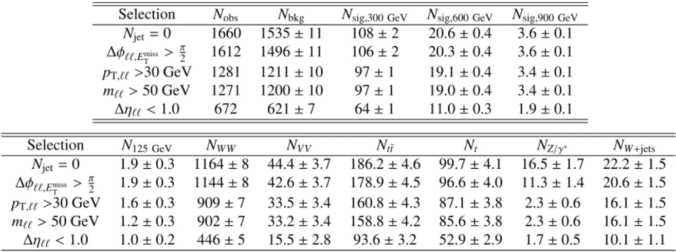
Table 3: Event yields for the N

= 0 final state. The top table compares the observed yields with the total background expectation and signal yields for m

= 300 GeV, 600 GeV and 900 GeV states with the SM lineshape after the application of the various selection criteria. The ggF and VBF production modes are added together. The bottom table shows the composition of the background. The require- ments are imposed sequentially from top to bottom. The quoted uncertainties represent the statistical uncertainties of the MC simulation.

Selection Nobs Nbkg Nsig,300 GeV Nsig,600 GeV Nsig,900 GeV

Njet=0 1660 1535±11 108±2 20.6±0.4 3.6±0.1

∆φ_``,Emiss

T >^π₂ 1612 1496±11 106±2 20.3±0.4 3.6±0.1

pT,`` >30 GeV 1281 1211±10 97±1 19.1±0.4 3.4±0.1

m_``>50 GeV 1271 1200±10 97±1 19.0±0.4 3.4±0.1

∆η_``<1.0 672 621±7 64±1 11.0±0.3 1.9±0.1

Selection N_{125 GeV} N_WW N_VV Nt¯t N_t N_Z/γ^∗ N_W+jets

Njet=0 1.9±0.3 1164±8 44.4±3.7 186.2±4.6 99.7±4.1 16.5±1.7 22.2±1.5

∆φ_``,Emiss

T >^π₂ 1.9±0.3 1144±8 42.6±3.7 178.9±4.5 96.6±4.0 11.3±1.4 20.6±1.5

pT,`` >30 GeV 1.6±0.3 909±7 33.5±3.4 160.8±4.3 87.1±3.8 2.3±0.6 16.1±1.5

m``>50 GeV 1.2±0.3 902±7 33.2±3.4 158.8±4.2 85.6±3.8 2.3±0.6 16.1±1.5

∆η_``<1.0 1.0±0.2 446±5 15.5±2.8 93.6±3.2 52.9±2.9 1.7±0.5 10.1±1.1

The methodology used to derive results has been detailed in Refs. [69,83]. The likelihood function

L is defined using the m

distribution for events after the selections in each final state. The m

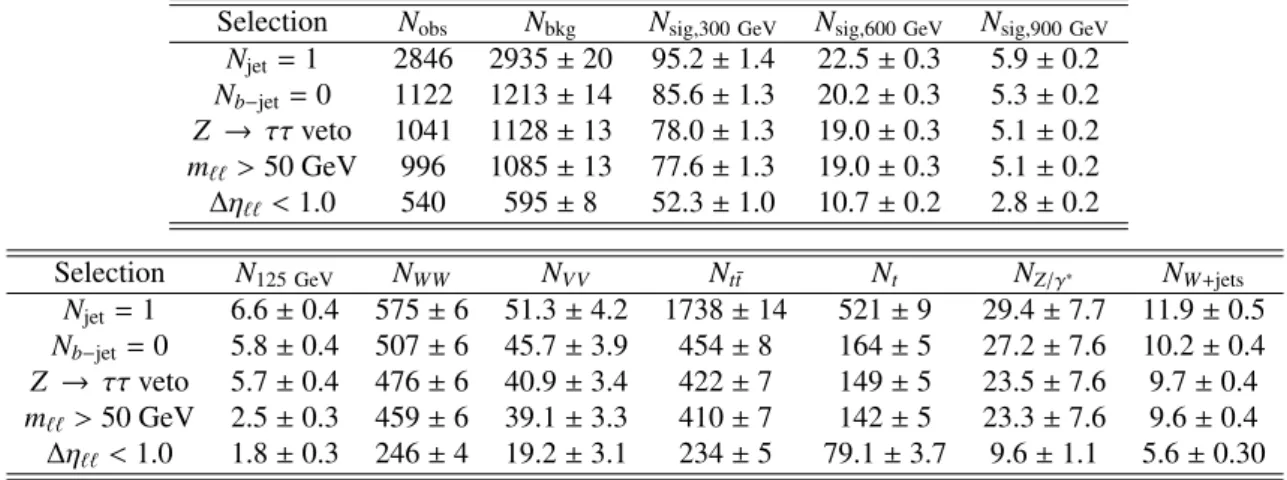
Table 4: Event yields for the N

= 1 final state. The top table compares the observed yields with the total background expectation and signal yields for m

= 300 GeV, 600 GeV and 900 GeV states with the SM lineshape after the application of the various selection criteria. The ggF and VBF production modes are added together. The bottom table shows the composition of the background. The require- ments are imposed sequentially from top to bottom. The quoted uncertainties represent the statistical uncertainties of the MC simulation.

Selection Nobs Nbkg Nsig,300 GeV Nsig,600 GeV Nsig,900 GeV

N_jet=1 2846 2935±20 95.2±1.4 22.5±0.3 5.9±0.2 Nb−jet=0 1122 1213±14 85.6±1.3 20.2±0.3 5.3±0.2 Z → ττveto 1041 1128±13 78.0±1.3 19.0±0.3 5.1±0.2 m``>50 GeV 996 1085±13 77.6±1.3 19.0±0.3 5.1±0.2

∆η``<1.0 540 595±8 52.3±1.0 10.7±0.2 2.8±0.2

Selection N125 GeV NWW NVV Nt¯t Nt NZ/γ^∗ NW+jets

Njet =1 6.6±0.4 575±6 51.3±4.2 1738±14 521±9 29.4±7.7 11.9±0.5 Nb−jet =0 5.8±0.4 507±6 45.7±3.9 454±8 164±5 27.2±7.6 10.2±0.4 Z → ττveto 5.7±0.4 476±6 40.9±3.4 422±7 149±5 23.5±7.6 9.7±0.4 m``>50 GeV 2.5±0.3 459±6 39.1±3.3 410±7 142±5 23.3±7.6 9.6±0.4

∆η_``<1.0 1.8±0.3 246±4 19.2±3.1 234±5 79.1±3.7 9.6±1.1 5.6±0.30

distributions in the signal regions are divided into twenty, ten, and four bins, respectively, for N

= 0, 1 and ≥ 2. The bins are of variable widths to have the same number of expected background events in each bin. L is a product of Poisson functions over the bins of the m

distribution in the signal and control regions. Each systematic uncertainty is parametrised by a corresponding nuisance parameter θ (its collection is θ) that is constrained by a Gaussian function. The parametrisations are implemented as log-normal distributions in order to prevent the nuisance parameters from taking unphysical values.

The modified frequentist method known as CL

[84, 85] is used to compute 95% CL exclusion limits. The method uses a test statistic q

, a function of the signal strength µ which is defined as the ratio of the measured cross section times branching ratio to that predicted. The test statistic is defined as:

q

= − 2 ln L(µ; ˆ θ

)/L( ˆ µ; ˆ θ)

(1) The denominator does not depend on µ. The quantities ˆ µ and ˆ θ are the values of µ and θ, respectively, that unconditionally maximise L. The numerator depends on the values ˆ θ

that maximise L for a given value of µ.

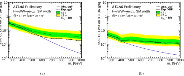
Figure 5 shows 95% CL upper limits on the production cross sections times branching ratio for H→WW →`ν`ν (with ` = e, µ, τ including all τ decay modes) for a SM-like scalar as a function of mass. Figure 6 shows upper limits on the production cross sections times branching ratio for a scalar with a narrow lineshape (NWA). To allow for constraints on a new resonance which may have di ff erent production rates in the ggF and VBF modes, the upper limits are estimated separately for the ggF and VBF production mechanisms. In each case, the parameters associated with the other production mechanism are treated as nuisance parameters in the likelihood fit.

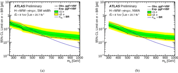
Figure 7 shows 95% CL upper limits on the production cross sections times branching ratio for

H→WW →`ν`ν (with ` = e, µ, τ including all τ decay modes), with both ggF and VBF production

modes treated as signal contributions, for the SM-like and NWA cases. In both cases, the SM values

of the ggF and VBF cross sections are used. A Higgs boson with a SM-like lineshape is excluded in

the range 260 GeV < m

< 642 GeV at 95% CL.

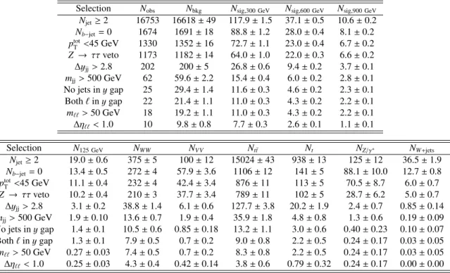
Table 5: Event yields for the N

≥ 2 final state. The top table compares the observed yields with the total background expectation and signal yields for m

= 300 GeV, 600 GeV and 900 GeV states with the SM lineshape after the application of the various selection criteria. The ggF and VBF production modes are added together. The bottom table shows the composition of the background. The require- ments are imposed sequentially from top to bottom. The quoted uncertainties represent the statistical uncertainties of the MC simulation.

Selection Nobs Nbkg Nsig,300 GeV Nsig,600 GeV Nsig,900 GeV

Njet≥2 16753 16618±49 117.9±1.5 37.1±0.5 10.6±0.2 Nb−jet=0 1674 1691±18 88.8±1.2 28.0±0.4 8.1±0.2

p^tot_T <45 GeV 1330 1352±16 72.7±1.1 23.0±0.4 6.7±0.2

Z → ττveto 1173 1182±14 64.0±1.0 22.0±0.3 6.6±0.2

∆yjj>2.8 202 200±5 26.8±0.6 9.4±0.2 3.7±0.1 mjj>500 GeV 62 59.6±2.2 15.4±0.4 6.0±0.2 2.8±0.1 No jets inygap 25 29.4±1.4 11.6±0.3 4.6±0.2 2.3±0.1 Both`inygap 22 21.4±1.1 11.0±0.3 4.3±0.2 2.2±0.1 m``>50 GeV 18 19.2±1.1 11.0±0.3 4.3±0.2 2.2±0.1

∆η``<1.0 10 9.8±0.8 7.7±0.3 2.6±0.1 1.1±0.1

Selection N125 GeV NWW NVV Nt¯t Nt NZ/γ^∗ NW+jets

Njet≥2 19.0±0.6 375±5 100±12 15024±43 938±13 125±12 36.5±1.9 Nb−jet=0 13.4±0.5 272±4 57.9±3.6 1106±12 141±5 88.1±10.0 12.7±0.8

p^tot_T <45 GeV 11.1±0.4 232±4 42.4±3.4 876±11 113±5 70.5±8.7 6.0±0.7

Z → ττveto 10.2±0.4 210±3 37.7±3.4 789±11 102±5 28.7±6.2 5.0±0.7

∆yjj>2.8 3.1±0.2 38.8±1.4 6.1±0.6 127.7±3.8 20.2±1.9 2.4±0.7 0.85±0.14 mjj>500 GeV 1.9±0.10 13.6±0.7 1.9±0.4 35.9±1.8 4.8±0.8 1.3±0.6 0.19±0.09 No jets inygap 1.4±0.1 10.5±0.6 0.85±0.18 13.2±1.1 3.0±0.6 0.40±0.23 0.10±0.07 Both`inygap 1.3±0.1 7.9±0.5 0.7±0.2 9.0±0.8 2.2±0.5 0.24±0.17 0.03±0.05 m``>50 GeV 0.27±0.03 7.4±0.5 0.7±0.2 8.3±0.8 2.2±0.5 0.24±0.17 0.03±0.05

∆η``<1.0 0.25±0.03 4.3±0.4 0.42±0.14 3.8±0.6 0.79±0.32 0.24±0.17 0.00±0.00

Table 6 shows the 95% CL upper limits on production cross sections times branching ratio for H→WW →`ν`ν (with ` = e, µ, τ including all τ decay modes) for m

= 300 GeV, 600 GeV and 1 TeV, for both SM-like and narrow (NWA) signal lineshapes and for the ggF and VBF production modes separately.

8 Conclusion

A search for a high-mass Higgs boson in the H→WW →`ν`ν channel has been presented, in the range 260 GeV < m

< 1 TeV for a signal with a SM-like lineshape and in the range 300 GeV

< m

< 1 TeV for a signal with a narrow-width lineshape. The search uses 20.7 fb

of proton-

proton collision data at a centre-of-mass energy of 8 TeV collected by the ATLAS experiment at the

LHC. No significant excess of events is observed in the explored mass range. For a high-mass Higgs

boson with a SM-like lineshape produced via gluon fusion, 95% CL upper limits on the cross section

times branching ratio are set at 250 fb, 34 fb and 19 fb, respectively, for m

= 300 GeV, 600 GeV and

1 TeV. A Higgs boson with SM-like production cross section and couplings is excluded at 95% CL in

the range 260 GeV < m

< 642 GeV. For a high-mass Higgs boson with a narrow-width lineshape

produced via gluon fusion, 95% CL upper limits on the cross section times branching ratio are 230 fb,

32 fb and 29 fb, respectively, for m

= 300 GeV, 600 GeV and 1 TeV.

[GeV]

mH

300 400 500 600 700 800 900 1000

BR [pb]×σ95% CL Limit on

10-3

10-2

10-1

1 10

Obs. ggF Exp. ggF

σ

±1 σ

±2

× BR σTh

Ldt = 20.7 fb-1

∫

= 8 TeV s

ATLAS Preliminary , SM width ν

µ ν

→e

→WW H

(a)

[GeV]

mH

300 400 500 600 700 800 900 1000

BR [pb]×σ95% CL Limit on

10-3

10-2

10-1

1 10

Obs. VBF Exp. VBF

σ

±1 σ

±2

× BR σTh

Ldt = 20.7 fb-1

∫

= 8 TeV s

ATLAS Preliminary , SM width ν

µ ν

→e

→WW H

(b)

Figure 5: 95% CL upper limits on the Higgs boson production cross section times branching ratio for H→WW →`ν`ν (with ` = e, µ, τ including all τ decay modes) for a Higgs boson with a SM-like lineshape. The limits are shown for (a) ggF production and (b) VBF production. The green and yellow bands show the ±1σ and ±2σ uncertainties on the expected limit. The expected cross section times branching ratio for the production of a SM Higgs boson is shown as a blue line.

[GeV]

mH

300 400 500 600 700 800 900 1000

BR [pb]×σ95% CL Limit on

10-3

10-2

10-1

1 10

Obs. ggF Exp. ggF

σ

±1 σ

±2

× BR σTh

Ldt = 20.7 fb-1

∫

= 8 TeV s

ATLAS Preliminary , NWA ν µ ν

→e

→WW H

(a)

[GeV]

mH

300 400 500 600 700 800 900 1000

BR [pb]×σ95% CL Limit on

10-3

10-2

10-1

1 10

Obs. VBF Exp. VBF

σ

±1 σ

±2

× BR σTh

Ldt = 20.7 fb-1

∫

= 8 TeV s

ATLAS Preliminary , NWA ν µ ν

→e

→WW H

(b)

Figure 6: 95% CL upper limits on the Higgs boson production cross section times branching ratio

for H→WW →`ν`ν (with ` = e, µ, τ including all τ decay modes) for a Higgs boson with a narrow

lineshape (NWA). The limits are shown for (a) ggF production and (b) VBF production. The green

and yellow bands show the ± 1σ and ± 2σ uncertainties on the expected limit. The expected cross

section times branching ratio for the production of a SM Higgs boson is shown as a blue line.

[GeV]

mH

300 400 500 600 700 800 900 1000

BR [pb]×σ95% CL Limit on

10-3

10-2

10-1

1 10

Obs. ggF+VBF Exp. ggF+VBF

σ

±1 σ

±2

× BR σTh

Ldt = 20.7 fb-1

∫

= 8 TeV s

ATLAS Preliminary , SM width ν

µ ν

→e

→WW H

(a)

[GeV]

mH

300 400 500 600 700 800 900 1000

BR [pb]×σ95% CL Limit on

10-3

10-2

10-1

1 10

Obs. ggF+VBF Exp. ggF+VBF

σ

±1 σ

±2

× BR σTh

Ldt = 20.7 fb-1

∫

= 8 TeV s

ATLAS Preliminary , NWA ν µ ν

→e

→WW H

(b)

Figure 7: 95% CL upper limits on the Higgs boson production cross section times branching ratio for H→WW →`ν`ν (with ` = e, µ, τ including all τ decay modes) for a Higgs boson with (a) a SM-like lineshape and (b) a narrow lineshape (NWA). The ggF and VBF production modes are both treated as signal contributions. The green and yellow bands show the ±1σ and ±2σ uncertainties on the expected limit. The expected cross section times branching ratio for the production of a SM Higgs boson is shown as a blue line.

Table 6: Observed 95% CL upper limits on σ · B (H→WW →`ν`ν with ` = e, µ, τ including all τ decay modes) corresponding to mass hypotheses of 300 GeV, 600 GeV and 1 TeV for a Higgs boson with a SM-like and a scalar with a narrow (NWA) lineshapes.

σ · B (fb)

Lineshape Production mode m

= 300 GeV m

= 600 GeV m

= 1 TeV

SM-like ggF 250 34 19

VBF 40 16 10

NWA ggF 230 32 29

VBF 39 12 10