Search for the Higgs boson in the process pp → W H → (`ν )(b ¯ b) with Run 2 data of the ATLAS experiment at the LHC Suche nach dem Higgs-Boson im Prozess

Search for the Higgs boson in the process pp → W H → (`ν )(b ¯ b) with Run 2 data of the ATLAS experiment at the LHC Suche nach dem Higgs-Boson im Prozess

pp → W H → (`ν )(b ¯ b) mit Run-2-Daten des ATLAS-Experiments am LHC

Master thesis submitted to

LMU Munich

by

Ilona Weimer

Born on 7

of May, 1987 in Frankfurt a.M.

Examiner: Prof. Dr. Otmar Biebel Co-examiner: Dr. Sandra Kortner

Munich, 2016

Abstract

The Higgs boson with a mass of 125 GeV was discovered in 2012 with the ATLAS and CMS experiments at the Large Hadron Collider. The decay of the Higgs boson in a bottom quark-antiquark pair has the highest branching ratio. However, the Higgs boson could not be detected yet in this decay channel due to the large contribution of background processes. A new approach for the improvement of the signal significance in search for H → b ¯ b decays produced in association with the W boson, is the so- called Higgs boson tagging. If the Higgs boson is produced with a large transverse momentum, the two b-quarks from the Higgs boson decay are strongly collimated and can be reconstructed as a single large jet. By applying specific requirements on the properties of the large jet and the substructure of the large jet, such as their invariant mass and the substructure, background processes can be efficiently suppressed. The analysis presented in this thesis is based on 3.2 fb

1 proton-proton collision data recorded by the ATLAS detector at a center-of-mass energy of 13 TeV.

Different substructure properties are tested in order to improve the tagging of large

jets from Higgs boson decays in regions of moderate Higgs boson transverse momenta

above 250 GeV. In the search for the pp → W H → (`ν)(b ¯ b) process, an improvement

of the signal significance by 33.6% is achieved in final states with at least three jets,

while the total improvement is 12.5%.

Contents

1. Introduction 1

2. Theoretical Background 3

2.1. The Standard Model . . . . 3

2.2. The Higgs mechanism . . . . 5

2.3. Higgs boson production and decays at the LHC . . . . 8

3. The ATLAS experiment at the LHC 15 3.1. The Large Hadron Collider at CERN . . . 15

3.2. The ATLAS detector . . . 18

3.2.1. The ATLAS coordinate system . . . 19

3.2.2. The Inner Detector . . . 21

3.2.3. The Calorimeter System . . . 22

3.2.4. The Muon Spectrometer . . . 25

3.3. Reconstruction of particles in the ATLAS detector . . . 26

4. Search for the Higgs boson in the process pp → W H → (`ν )(b ¯ b) 31 4.1. Signal and background events . . . 31

4.2. Event selection . . . 34

4.3. Results . . . 40

5. Study of signal events with large-size jets 47 6. W H Analysis optimization based on the jet substructure 53 6.1. Jet substructure variables . . . 53

6.2. Analysis optimization by means of substructure variables . . . 58

6.3. Correlations between substructure variables . . . 70

7. Summary and outlook 73

A. Distributions of topological and kinematical variables at various stages

of event selection 75

B. Higgs boson tagger 80

List of Figures 91

Selbstst¨ andigkeitserkl¨ arung 95

1. Introduction

With the discovery of the Higgs boson in 2012 with the ATLAS and CMS experi- ments at the LHC, the Standard Model of elementary particles was complete. Since then, the measurement of the Higgs boson properties and the detection of the Higgs boson in all theoretically predicted production and decay channels becomes an im- portant field in particle physics. The decay of a Higgs boson with a mass of 125 GeV into a bottom quark anti-quark pair is predicted to have the highest branching ratio of all Higgs boson decay modes. However, there is still no evidence for H → b ¯ b decays because of the large background contamination. The Higgs boson decays into bottom quark-antiquark pairs are typically examined in associated Higgs boson production with vector bosons or top-quark pairs, as the electrons or muons from the decay of the associate particle have a clear signature in the detector and can be used for a better discrimination between signal and background events.

In this analysis, the associated Higgs boson production with a W boson decaying into a charged lepton and a neutrino pp → W H → (`ν)(b ¯ b), is examined. The analysis is based on Run 2 data recorded by the ATLAS detector in 2015 at a centre- of-mass energy of 13 TeV. The properties of the signal and background processes are studied. In particular, different jet properties are examined with the aim to suppress the contamination from background processes. For a Higgs boson produced with a sufficiently high momentum, the two b-jets from its H → b ¯ b decay are collimated. Thus, they may be reconstructed as one large jet instead of two smaller jets. The substructure of such a large jet can serve as a major handle for background suppression. A variety of substructure variables is tested as possible discriminants against the background in order to optimize the signal significance.

In the following chapter, the Standard Model of elementary particles, the Higgs mechanism and the phenomenological properties of the Higgs boson are presented.

Chapter 3 gives an overview of the Large Hadron Collider and the ATLAS exper-

iment. Furthermore, the reconstruction of particles by the ATLAS detector is de-

scribed. In Chapter 4, the signal and dominant background processes are presented.

The nominal selection of pp → W H → (`ν)(b ¯ b) events with specific requirements

on the reconstructed objects and their topological and kinematic properties is ap-

plied on signal and background events to reduce the background contribution. In

Chapter 5, the tagging of large jets from H → b ¯ b decays is introduced as a possible

discriminant against the background contribution. In Chapter 6, the substructure

of the large jets that are tagged as H → b ¯ b decays are presented. Additional re-

quirements are applied on the most discriminating substructure variables in order

to improve the analysis sensitivity. The results of the study are summarized in

Chapter 7.

2. Theoretical Background

2.1. The Standard Model

The Standard Model of elementary particles is a quantum field theory based on local gauge symmetries. It is represented by the symmetry group

SU(3) ⊗ SU(2)

⊗ U (1)

, (2.1)

where SU (3) describes the strong interaction and SU (2)

⊗ U (1)

the electroweak interaction. The subscript “L” indicates that the group acts only on the left-handed components of the spinor of elementary fermions. Subscript “Y” is the hypercharge, relating the strong interactions of the SU (3) model.

There are three fundamental interactions which are described by local quantum gauge field theories, as summarized in Table 2.1.

Table 2.1.: The three fundamental interactions of the Standard Model with their couplings and force carriers with corresponding mass and J

, where J denotes the spin and P the parity of the particle.

Interaction Couples to Force carriers Mass (GeV) J

Electromagnetic Electric charge Photon (γ) 0 1

Weak Weak charge W

, Z

≈ 10

1

Strong Colour 8 gluons (g) 0 1

• Quantum electrodynamics (QED) [1, 2]: Particles carrying electrical

charge interact electromagnetically. The massless photon is the mediator of the

electromagnetic interaction. The group properties are defined by the Abelian

group U (1).

• Weak interaction [3–6]: The weak interaction is mediated by the massive W

, W

and Z

bosons.

• Quantum chromodynamics (QCD) [7]: Particles with colour charge inter- act via the strong interaction, mediated by eight massless gluons. As gluons carry colour, they interact among each other. QCD is defined by the non- Abelian SU (3) gauge group.

The elementary particles predicted by the Standard Model can be divided into two main groups, the fermions and the bosons. An overview of these particles can be seen in Figure 2.1.

Figure 2.1.: Overview of the Standard Model particles [8].

• Fermions are spin-1/2 particles. They can be classified in three generations with increasing mass. There are two types of fermions – quarks and leptons.

Leptons can be further divided into charged leptons (e

, µ

, τ

) and neutrinos

Table 2.2.: Overview of the fermions in the Standard Model.

Fermions Generation Electric Colour Weak isospin J

1 2 3 charge [e] left-handed right-handed

Leptons ν

ν

ν

0 — 1/2 — 1/2

e µ τ –1 — 1/2 0 1/2

Quarks u c t +2/3 r,b,g 1/2 0 1/2

d s b –1/3 r,b,g 1/2 0 1/2

(ν

, ν

, ν

). For each fermion there exists one anti-fermion with the same mass, but opposite electric charge and parity quantum number. Table 2.2 gives an overview of the Standard Model fermions with their main properties.

• Bosons carry integer spin. The fundamental interactions are mediated by spin-one vector bosons (eight gluons, the W

and Z

bosons and the photon).

In addition, there is one scalar spin-zero particle, the Higgs boson predicted by the Standard Model Higgs mechanism [9–11]. The W

and Z

bosons and the Higgs bosons are massive, while gluons and the photon are massless.

All particles predicted by the Standard Model have been experimentally observed and their properties and interactions extensively tested. All observations agree ex- tremely well with theoretical predictions. The properties of the most recently dis- covered Higgs boson at the Large Hadron Collider [12, 13], are also compatible with the Standard Model predictions [14, 15]. The precision of these measurements however still leaves room for deviations from the Standard Model and is constantly improving with new LHC data.

2.2. The Higgs mechanism

The Glashow-Salam-Weinberg model of electroweak interaction unifies the electro-

magnetic and weak forces with the gauge symmetry SU(2)

⊗ U (1). It contains

three vector fields of the SU (2)

group, W

(i = 1,2,3), and one of the U(1) group,

B

. The vector bosons W

, Z

and the photon are described as linear combinations

of these four vector fields,

W

= 1

√ 2 (W

∓ W

) Z

= W

· cos θ

− B

· sin θ

A

= W

· sin θ

+ B

· cos θ

.

(2.2)

The mixing is expressed as a rotation of the original W

and B

vector boson plane by an angle θ

, also called Weinberg angle, or weak mixing angle.

The gauge invariance of this theory is conserved only in case of massless gauge bosons. The observation of massive W

and Z bosons, however, contradicts to this assumption.

Peter Higgs and independently Robert Brout and Francois Englert solved this problem in 1964 by postulating the so-called Higgs mechanism [9–11], introducing the gauge boson masses via the spontaneous electroweak symmetry breaking.

In this model, a new complex scalar field is introduced, the so-called Higgs field.

At high temperatures (energies) the W

and Z bosons are massless, while below a certain energy they acquire mass via interaction with the Higgs field.

The potential of the Higgs field Φ is given by

V (Φ) = µ

Φ

Φ + λ|Φ

Φ|

. (2.3) where λ describes the strength of the quartic self-interaction and µ is a mass pa- rameter.

For λ > 0 and µ

< 0 the shape of the potential resembles a mexican hat (see Fig. 2.2). While for µ

> 0 the state of minimum energy is located at the origin (Φ

= 0), for µ

< 0 the minima lie on a circle away from the origin. This is an infinite set of degenerate ground states which satisfy the condition

Φ

Φ

= − µ

2λ ≡ v

2 , (2.4)

where v is the vacuum expectation value of the scalar field Φ. Choosing one of

the non-zero ground states leads to spontaneous breaking of the SU (2)

⊗ U (1)

symmetry.

Figure 2.2.: The Higgs potential [16].

With the choice of the ground state at Φ

= − 1

√ 2 0 v

!

, (2.5)

excitations of the Higgs field from the ground state can be written as Φ(x) = − e

√ 2

0 v + H(x)

!

, (2.6)

with four real scalar fields H(x) and θ

(x) (i = 1, 2, 3). H(x) corresponds to an excitation which changes the enrgy of the Higgs field manifesting itself as a new scalar particle - the Higgs boson. The W

and Z bosons acquire their mass bia their interaction with the field φ(x).

The gauge boson masses are related through the weak mixing angle θ

, m

= v

2 = m

cos θ

(2.7)

with v = 246 GeV [17]. Couplings between the Higgs boson H and the weak vector

bosons V = W

, Z are proportional to the squares of the boson masses m

. g

= −2i m

v and g

= −2i m

v

. (2.8)

Higgs boson couplings to fermions are proportional to the fermion masses m

. g

= √

2i m

v (2.9)

The Higgs boson mass is given by m

= √

2λv

. As λ is a free parameter of the theory, the value of m

is not predicted by the Standard Model and must be evaluated experimentally.

2.3. Higgs boson production and decays at the LHC

With the discovery of the Higgs boson with a mass of 125 GeV at the LHC, the only missing particle of the Standard Model appears to be found. In order to fully test the electroweak symmetry breaking mechanism, phenomenological properties of the Higgs boson and the measurement of different Higgs boson production and decay modes now become a crucial test of the Standard Model.

The phenomenology of the Standard Model Higgs boson is described in Ref. [18].

Being electrically neutral, the Higgs boson can couple to a fermion-antifermion pair, W

W

pair or to a ZZ pair. For a given Higgs boson mass all production and decay properties of the Higgs boson can be theoretically predicted.

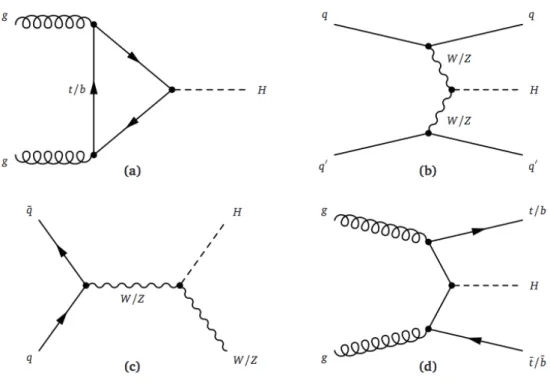
In Figure 2.3 the four main Higgs production modes in proton-proton collisions are illustrated. They all involve couplings of the Higgs boson to relatively heavy particles (W and Z bosons or top and bottom quarks) as the couplings to the Higgs boson are proportional to the particle masses. Although gluons do not couple directly to the Higgs boson, the gluon fusion (ggF) via heavy quark loops is one of the dominant production mechanisms, followed by about 10 times weaker production via vector boson fusion (VBF). These two mechanisms are followed by a production in association with a W or Z boson (V H), also called Higgs-strahlung, and associated production with a heavy top or bottom quark pair (t tH ¯ , b ¯ bH).

The cross sections for the Higgs boson production via the dominant production mechanisms at a center-of-mass energy of √

s = 13 TeV are summarised in Table 2.3.

As gluon fusion has the highest cross section, it is the most important production

Figure 2.3.: Feynman diagrams of the four most important Higgs boson production mechanisms: (a) gluon fusion (ggF), (b) vector boson fusion (VBF), (c) associated production with a W or Z boson (Higgs-strahlung, V H), and (d) associated production with a pair of heavy quarks (t ¯ tH or b ¯ bH).

mechanism for most decays.

Table 2.3.: Production cross section for the most important production modes of the Standard Model Higgs boson with a mass of 125 GeV at

√ s = 13 TeV [19].

Prod. mode ggF VBF WH ZH t ¯ tH b ¯ bH

σ [pb] 44.14 3.782 1.373 0.839 0.5071 0.4880

As the lifetime of the Higgs boson is relatively short compared to the size of the detector, it can be detected only through its decay products. The dominant decays are illustrated in Figure 2.5. The probablity for a certain decay is given by the branching ratio

BR(H → X) = Γ(H → X) P

Y

Γ(H → Y ) , (2.10)

where Γ(H → X) is the decay width for a given Higgs boson decay H → X and depends on the Higgs boson mass m

. The decay width to fermions is given in Born approximation as

Γ(H → f f ¯ ) = n

8v

π m

m

1 − 4m

m

, (2.11)

where n

is the colour factor (n

= 3 for quarks, n

= 1 for leptons) and m

the fermion mass [20].

The decay width to gauge bosons H → V V with V = (W or Z ) is given by Γ(H → V V ) = n

32v

π m

δ

√

1 − 4x(1 − 4x + 12x

), x = m

m

(2.12) with δ

= 2, δ

= 1 and the vector boson mass m

. The partial width of a Higgs boson decaying into two photons can be written in leading order as

Γ(H → γγ) = α

256v

π

| X

f

n

Q

A

(τ

) + A

(τ

)|

(2.13)

with the fine-structure constant α and the form factors for spin-1 and spin-1/2 particles

A

(τ

) = 2 (τ

+ (τ

− 1)f(τ

)) τ

and A

(τ

) = − 2τ

+ 3τ

+ 3(2τ

− 1)f(τ

)

τ

,

(2.14)

respectively. The function f(τ

) is defined as f (τ

) = arcsin

√

τ

for τ

≤ 1 f (τ

) = − 1

4 log 1 + p

1 − τ

1 − p

1 − τ

− iπ

!

for τ

> 1 (2.15)

where τ

= m

/4m

with i = f, W .

Figure 2.4 shows the branching ratios for the different decay modes as a function

of the Higgs boson mass [19]. In Table 2.4 the values for m

= 125 GeV are sum-

marized. The dominant decay mode for the observed Higgs boson mass is the decay

to a b-quark-antiquark-pair, followed by the decay to a W -boson-pair. All other

branching ratios are significantly lower. In the following each decay is addressed

shortly.

Figure 2.4.: Branching ratios for Standard Model Higgs boson decays and their uncertainties as a function of the Higgs boson mass m

[19].

Figure 2.5.: Feynman diagrams for the dominant Higgs boson decays into (a) two

photons, (b) a pair of vector bosons and (c) a pair of fermions.

Table 2.4.: Branching ratios for the different decays of a Standard Model Higgs boson with a mass of 125 GeV [19].

Decay mode Branching ratio (m

= 125 GeV)

H → b ¯ b 58.24 %

H → W W 21.37 %

H → gg 8.19 %

H → τ

τ

6.27 %

H → c¯ c 2.89 %

H → ZZ 2.62 %

H → γγ 0.228 %

H → Zγ 0.154 %

H → µ

µ

0.0219 %

• H → b ¯ b: A Higgs boson with a mass of 125 GeV decays most probably to a pair of bottom quarks. The detection of this decay mode is difficult due to a large background contamination. The two b-quarks from the Higgs boson decay hadronize, resulting in a final state with two b-jets from the hadron- induced particle showers in the detector. A similar final state is also obtained in an order of magnitudes more frequent multijet production. For this reason, the H → b ¯ b decay can only be detected in associated production with vector bosons or top quark pairs. The electrons or muons from the vector boson or top quark decay serve as a powerful handle for background suppression.

• H → W W : This bosonic decay mode has the second highest branching ratio.

The Higgs boson decays into two W bosons can best be observed in final states in which both W bosons further decay to one charged lepton and one neutrino.

Because of the neutrinos in the final state, the precise reconstruction of the Higgs boson mass is difficult.

• H → gg and H → c¯ c: Because of high multijet background contributions, the detection of the Higgs boson is not possible in these decay modes.

• H → τ

τ

: The decay to a τ-pair is another channel with a high branching

ratio. The decays of Z bosons to τ -pairs and the multijet production are the

main irreducible and reducible backgrounds, respectively, in this decay mode.

• H → ZZ : The most sensitive search in this decay mode is performed in the final state where both Z bosons decay to a pair of electrons or muons. This is a very clean final state with low background contamination and a very good Higgs boson mass resolution.

• H → γγ: Although the branching ratio is small, the decay to two photons is a very important channel because of the very clean signal signature and a bery good Higgs boson mass resolution.

• H → µµ and H → Zγ: At the moment there is not enough data available to detect the Higgs boson in these decay modes.

In order to detect the Higgs boson and to study its properties, particle accelerators

with large collision energies are needed and are currently provided by the Large

Hadron Collider at CERN.

3. The ATLAS experiment at the LHC

3.1. The Large Hadron Collider at CERN

The Large Hadron Collider (LHC) [21] is a proton storage ring with a circumference of 26.7 km located at the European Organization for Nuclear Research (CERN) near Geneva. It collides proton beams circulating in evacuated pipes in opposite directions and is presently the machine with the highest centre-of-mass energy in particle physics. The LHC is designed to collide protons at a centre-of-mass energy of √

s = 14 TeV and a peak luminosity of 10

cm

s

. Further, collisions of heavy lead ions with 2.8 TeV per nucleon and 10

cm

s

are possible.

Several experiments are situated at the LHC, the main ones being ATLAS (A Toroidal LHC ApparatuS) [22], CMS (Compact Muon Solenoid) [23], LHCb (Large Hadron Collider beauty) [24] and ALICE (A Large Ion Collider Experiment) [25].

While LHCb is specialized on the study of CP violation and ALICE is dedicated to studies of the quark-gluon plasma using high-energetic collisions of lead ions, ATLAS and CMS are multi-purpose experiments designed amongst others for the search for the Higgs boson and physics beyond the Standard Model, such as supersymmetry and dark matter. An overview of the CERN accelerator comples and locations of the main experiments at the LHC can be seen in Figure 3.1. As this analysis is based on data taken with the ATLAS detector, this detector will be described in more detail in Section 3.2.

Before being injected into the LHC tunnel, the particles are accelerated in a chain

of pre-accelerators. At first, the valence electrons are stripped off hydrogen atoms

and the energy of the protons is increased to 50 MeV in the Linear accelerator 2

(LINAC2). Then they are further accelerated to 1.4 GeV in the Proton Synchrotron

Booster (PSB), to 25 GeV at the Proton Synchrotron (PS) and to 450 GeV at the

Super Proton Synchrotron (SPS) [26]. Finally, they are injected with this energy

Figure 3.1.: The CERN accelerators [27].

into the LHC, which is designed for a maximum energy of 7 TeV per proton beam.

The injections of the proton beams are executed in two opposite directions, so that collisions are possible at dedicated interaction points.

At the LHC, superconducting dipole magnets with currents of 11700 A are used to bend the paths of the particle beams in order to keep the particles on their orbits. The magnets are being cooled with liquid helium to -271.3

C. With this arrangement magnetic fields of 8 T can be achieved. In addition, quadrupol magnets are used to stabilize and focus the beams. The proton beam consists of about 2808 packages with 10

protons each, with collisions every 25 ns.

The event rate is given by dN/dt = Lσ, where σ is the cross section. It is determined by the luminosity

L = N

n

f

4πσ

· F (3.1)

where N

is the number of particles per bunch, n

the number of bunches per beam,

f

the revolution frequency of the protons, σ

the transverse root mean square

beam size at the interaction point and F a geometric reduction factor that takes

(a) (b)

Figure 3.2.: Cumulative luminosity versus time delivered to ATLAS during stable beams for high energy p-p collisions: (a) for 2011-2016, (b) for 2016, delivered to (green) and recorded by ATLAS (yellow) [28].

into account that the beams cross under an angle. The LHC is designed for a peak luminosity of 10

cm

s

.

For the physics research the integrated luminosity L = R

L dt collected over time is an important dimension. In 2016, the LHC delivered an integrated luminosity of 19.6 fb

at a collision energy of 13 TeV. Of these, 17.9 fb

were recorded by the ATLAS detector. Distributions of the integrated luminosity as a function of time can be seen in Figure 3.2.

For a given luminosity, the expected number of inelastic proton-proton collisions

per bunch crossing can be calculated. As the rates of most hard-scattering processes

of interest are small, these will in general be accompanied by processes additional

inelastic proton-proton collisions in the same event. If the additional collisions occur

in the same bunch crossing, this is referred to as in-time pile-up. Because of the

small bunch spacing of about 25 ns, also interactions from neighbouring events, the

so-called out-of-time pile-up can contribute. Further, proton interactions with the

detector material (cavern background) must be considered. Figure 3.3 shows the

distribution of the mean number of interactions per bunch crossing recorded with

the ATLAS detector in 2015 and 2016.

Figure 3.3.: Luminosity weighted distribution of the mean number of interactions per bunch crossing measured by the ATLAS detector in 2015 and 2016 [28].

3.2. The ATLAS detector

The ATLAS detector is a general purpose detector, designed for precision mea- surements of Standard Model processes, but also for the discovery of new physics processes with small cross sections, such as the Higgs boson production. It is 44 m long, 25 m wide and 25 m high, weighs around 7000 tons and is located about 100 m under the earth’s surface. Because of the cylindric form, the collision point in the middle is enclosed from all directions. A schematic view of the detector is given in Figure 3.4.

The ATLAS detector consists of cylindrical layers of detectors around the beam pipe and two endcap disks in the forward regions. There are three main detector subsystems: the inner detector, the calorimeter system and the myon spectrometer.

In order to reconstruct the proton-proton interactions at the large luminosity and high collision rate at the LHC, a very high spacial and time resolution is needed in each op these subsystems.

Each particle has a unique signature in one or more of the detector subsystems.

Position and energy measurements in different detectors provide information on the

type of the particle and its four-momentum. An illustration of the different particle

signatures in the ATLAS detector is shown in Figure 3.5.

Figure 3.4.: Schematic view of the ATLAS detector [22].

3.2.1. The ATLAS coordinate system

The ATLAS coordinate system is used to describe the position of measured collision deposits. The origin of the coordinate system is set at the proton-proton interaction point. The z axis points along the beam direction. The positive x axis points to the centre of the LHC ring and the positive y axis to the earth’s surface.

The ATLAS barrel region is invariant under discrete rotations around the beam axis and furthermore has a forward-backward symmetry. For this reason, a cylin- drical coordinate system is often used. The azimuthal angle φ is measured in the x-y-plane around the beam axis z, starting from the positive x axis. The polar angle θ is defined as the angle with respect to the positive z axis. Instead of θ, usually the pseudorapidity

η = − ln

tan θ

2

(3.2) is used, as it is invariant under longitudinal boosts of particles in z-direction. For massive objects, the rapidity

y = 1 2 ln

E + p

E − p

(3.3)

is used. For high E/m values, the pseudorapidity and the rapidity are equal. An-

Figure 3.5.: Illustration of signatures of different particles in the ATLAS detec-

tor [29].

other important parameter is the angular separation between two objects, charac- terized by the distance parameter

∆R = p

∆η

+ ∆φ

= p

(η

− η

)

+ (φ

+ φ

)

. (3.4) If parameters such as momentum, mass or energy are measured only in the x-y- plane, they are referred to as transverse momentum

p

= q

p

+ p

= |p|

cosh η , (3.5)

transverse energy

E

= E

cosh η (3.6)

or transverse mass

m

= s

X

i

E

− X

i

p

. (3.7)

3.2.2. The Inner Detector

The Inner Detector (ID), 6.2 m long and 2.1 m high, is the innermost layer of the ATLAS detector. A cut-away view of the Inner Detector is shown in Figure 3.6.

The middle sector with cylindric detectors (barrel region) is closed at both sides by endcap disks. The ID measures the trajectories (tracks) of the charged particles produced in the collision as well as their vertex position. It is located in a solenoidal magnetic field. Charged particles traversing the detector are bent in a magnetic field of 2 T, so that their transverse momenta can be measured. At the LHC design luminosity there are 100 tracks produced per bunch-crossing are produced on aver- age, leading to a very high track density in the inner detectors. Thus a very fine granularity is needed in order to cope with the high density. It is achieved by three ID subdetectors.

The Pixel Detector is the innermost part of the ID. It is covering pseudorapidity values of |η| < 2.5 and consists of silicon pixel detectors. Because the distance to the collision point is small, the number of particles per time and area is very high, calling for a very fine granularity. The pixel detector has more than 80 million readout channels and on average performs three measurements per charged particle.

It has a spatial resolution of 10 µm in the r-φ plane and 115 µm along the z axis.

The silicon sensors are placed in three cylindrical layers in the barrel and in disks in

the endcap region. As the innermost layer of the pixel detector is very important for the identification of b quarks, it is also called the B-Layer. An additional Insertable B-Layer (IBL) with a reduced pixel size, a CO

-based cooling system and new carbon foam structures was installed as the fourth innermost layer in Run 2 [? ].

The Semiconductor Tracker (SCT) is also a silicon detector and surrounds the pixel detector. It extends up to |η| < 2.5 and consists of four cylindrical layers of silicon strip sensors in the barrel and nine disks in each endcap. The sensor strips are arranged under small angles along the beam line, so that the measurement of the the z-coordinate is possible. The spatial resolution is smaller than in the pixel detector, as the readout is performed per stripe. There are around 6 million readout channels.

Between 4 and 9 measurements per particle are made. Particles are localized with a precision of 17 µm in the transverse plane and 580 µm along the z-axis.

The Transition Radiation Tracker (TRT) is the outermost layer of the ID. It has around 351000 readout channels. The straw tubes are 4 mm in diameter with 31 µm gold plated tungsten anode wires in their center. They are filled with a gas mixture (70% Xe, 27% CO

, 3% O

). The TRT is covering angles of |η| < 2.0 and has a spatial resolution of about 130 µm in the r-φ plane. Along the z axis it does not provide measurements. Traversing charged particles on average hit 36 straw tubes.

3.2.3. The Calorimeter System

The next layer in the ATLAS detector is the calorimeter system, extending up to η ≤ 4.9 and consisting of the electromagnetic and the hadronic calorimeter. A cut- away view of the calorimeter system can be seen in Figure 3.7. The electromagnetic calorimeter is located outside a solenoid coil surrounding the ID. It serves for the identification of electrons and photons by measuring their energy and direction. The hadronic calorimeter measures the energy of hadrons and jets. Both calorimeters consist of alternating layers of passive absorber material and of active material mea- suring the energy deposition of incoming particles. Hadrons, electrons and photons are completely stopped in the calorimeters.

The barrel part of the Electromagnetic Calorimeter is 6.4 m long and 1.2

m high and weighs 114 t. It extends up to |η| < 3.2. The electromagnetic disk

calorimeters at both endcaps (EMEC) are 63 cm thick and 177 cm high and cover the

pseudorapidity region of 1.4 < |η| < 3.2. The active material is liquid argon (LAr),

while lead is used as absorber material. Traversing electrons and photons radiate

Figure 3.6.: Cut-away view of the ATLAS Inner Detector (ID) [22].

photons and build electron-positron-pairs in a decelerating showering process, and are finally fully absorbed.

A very fine granularity in the region up to |η| ≤ 2.5 allows for an accurate measurement of the direction of electrons and positrons can be measured very ac- curately. The granularity in the region |η| ≥ 2.5 is coarser, but still sufficient for the measurement of the missing transverse energy and for the jet reconstruc- tion. The electromagnetic calorimeter is designed for a resolution of σ(E)/E = 10%/ p

E[GeV] ⊕ 0.7%, where E is the energy of the traversing particle.

The Hadronic Calorimeter surrounds the electromagnetic calorimeter. The barrel part is 5.8 m long, with two extended barrels, each 2.6 m long and 1.97 m high. Hadrons are not stopped in the electromagnetic calorimeter, but deposit most of their energy in the hadronic calorimeter, which consists of three parts:

the Tile Calorimeter, the Hadronic Endcap Calorimeter (HEC) and the Forward

CALorimeter (FCAL). Through interactions in the absorber layers, the hadrons

produce showers of electrons and photons which are detected in the scintillator

layers. The reconstructed showers are referred to as jets. The Tile Calorimeter

covers the region |η| < 1.0, with extensions to |η| < 1.7. It consists of alternating

layers of steel absorbers and scintillators. The hadronic endcap calorimeter (HEC)

Figure 3.7.: Schematic view of the ATLAS calorimeter system with an electromag-

netic (EMEC) and a hadronic (HEC) calorimeter in the endcaps as

well as a thinner electromagnetic calorimeter with liquid Argon (LAr)

and a thicker hadronic tile-calorimeter [22].

Figure 3.8.: Schematic view of the ATLAS Muon Spectrometer. The system con- sists of four detector technologies: Monitored Drift Tubes (MDT), Cathode Strip Chambers (CSC), Resistive Plate Chambers (RPC) and Thin Gap Chambers (TGC) [22].

uses liquid argon as active material and copper as absorber. It covers the region 1.5 < |η| < 3.2. The liquid argon Forward CALorimeter (FCAL) is built of three consecutive modules in z-direction in each endcap and covers the region 3.1 < |η| <

4.9. As absorber material copper (module closest to the interaction region) and tungsten (other two modules) are used. For the hadronic calorimeter, a resolution of σ(E)/E = 50%/ p

E[GeV] ⊕ 3% is required in the barrel and the endcaps, while in forward direction it can be reduced to σ(E)/E = 100%/ p

E[GeV] ⊕ 10%.

3.2.4. The Muon Spectrometer

The Muon Spectrometer (MS) is the outermost layer of the ATLAS detector. It is

designed to identify muons and to precisely measure their momenta. It extends up

to |η| ≤ 2.7. Muons with transverse momenta above 3 GeV reach the MS and are

bent in the 0.3 - 1.2 T magnetic field of superconducting air-core toroid magnets.

A big barrel toroid is providing the magnetic field for |η| ≤ 1.4, while two endcap toroids are covering the region 1.6 < |η| < 2.7. In the region of 1.6 < |η| < 2.7, also referred to as transition region, the fields of the barrel and endcap toroids overlap, so that the magnetic field is relatively inhomogeneous. A schematic view of the Muon Spectrometer is shown in Figure 3.8.

Four different detector technologies are installed in this subsystem: Monitored Drift Tube chambers (MDT), Cathode Strip Chambers (CSC), Resistibe Plate Chambers (RPC) and Thin Gap Chambers (TGC). The precision tracking chambers MDT and CSC are arranged in the barrel part in three cylindrical layers at radii of around 5 m, 7.5 m and 10 m around the beam axis, and in the endcap part in three layers of round disks vertical to the beam axis at distances of 7.4 m, 10.8 m, 14 m and 21.5 m. The MDT chambers consist of aluminum drift tubes with a diameter of 30 mm and are filled with a gas mixture (93% Argon, 7% CO

) at a pressure of 3 bar. The CSC, located between the endcap toroids, are multi-wire proportional precision tracking chambers with cathodes segmented into strips. They are filled with a gas mixture (30% Argon, 50% CO

, 20% CF

). The muon transverse mo- mentum resolution provided by the precision tracking chamber is in the transverse momentum range of 10 - 1000 GeV.

The muon trigger system consists of the RPC in the barrel and the TGC in the endcaps, covering the region |η| < 2.4. In addition to fast muon trigger decision, they provide measurements orthogonal to the direction provided by the precision chambers, allowing for a more precise track reconstruction.

3.3. Reconstruction of particles in the ATLAS detector

In this section the reconstruction of particles relevant for this analysis are described.

When traversing the inner detector, charged particles leave collections of clustered

hits. These are reconstructed as particle tracks. Leptons (electrons and muons) and

jets are reconstructed with dedicated algorithms and identified by specific selection

criteria based on the the ID tracks and additional information they deposit in the

calorimeters and the MS.

Electron reconstruction

Electrons are reconstructed from noise-suppressed calorimeter energy clusters [30].

A sliding window algorithm is used for the cluster finding and a matching charged ID track is required in addition. Electron candidates must fulfill criteria on the electromagnetic shower shape and the quality of the track reconstruction and the track-cluster matching. A likelihood-based approach is used to combine these re- quirements and provide the electron identification. An isolation criterion is defined using requirements on the sum of the transverse momenta of the trajectories located in a cone around the electron direction, where the radius of the cone is a function of the electron transverse momentum. Based on the identification efficiency, there are three working points available: loose, medium and tight identification, ranked with decreasing contamination of misidentified objects. Loose electrons fulfill the basic requirements listed above and have p

> 7 GeV and |η| < 2.47. Medium electrons pass the same requirements as loose electrons and are further required to have p

> 25. Tight electrons pass the medium selection and in addition tighter requirements on the likelihood and isolation from jet activity to further suppress backgrounds. The electron energies are calibrated using reference processes such as Z → ee, which are measured in the data.

Muon reconstruction

Muons are reconstructed from the hits deposited in the inner detector and the muon spectrometer [31]. As for electrons, an isolation criterion is defined using the sum of the transverse momenta of the trajectories located in a cone around the muon direction and three working points are defined with increasing purity of true muons.

Loose muons pass basic requirements on muon track parameters and isolation and have p

> 7 GeV and |η| < 2.5. Medium muons in addition have p

> 25 GeV.

Tight muons fulfill the medium criteria and additionally tighter identification and isolation requirements. The muon energies are calibrated using the Z → µµ decay as a reference processes.

Jet reconstruction

For the jet reconstruction [32] noise-suppressed clusters of energy in the calorimeter

are used as the input. The nominal jets are reconstructed with the anti-k

algo-

rithm [33] with a radius parameter of R = 0.4. In order to calibrate the energies

of reconstructed jets, both simulation-based correction factors and in-situ measure- ments from data are used [34]. Events with jets likely to originate from non-collision sources and noise are identified and removed. Further selection criteria are applied to jets with transverse momenta below 60 GeV and |η| < 2.4 in order to remove jets which are likely to have come from additional collisions within the same bunch crossing. The analysis defines two jet categories: forward jets are required to have p

> 30 GeV and 2.5 ≤ |η| ≤ 4.5, while signal jets must have p

> 20 GeV and

|η| < 2.5.

Tagging of b-jets

Jets originating from bottom quarks are identified using the MV2c20 [35] b-tagging algorithm at the 70% efficiency working point, so-called b-jets. The MV2c20 algo- rithm is a multivariate algorithm combining the IP3D, SV1 and JetFitter algorithms, which are using the ID trajectories of charged particles as an input. The b-tagging algorithm exploits the fact that b-quarks have a relatively long life-time, so that typically at least one vertex originating from B-hadron decays is shifted away from the primary vertex at the hard-scatter collision point. The energy of the jets tagged as b-jets is correlated to account for two effects. If the b-quark decays via the weak interaction, a muon can be produced in this process. The four-vector of this muon is measured by the muon reconstruction algorithm and added to the original jet four-momentum and the calorimeter energy deposits corresponding to the muon are removed. This correction is applied if at least one muon is matched to a jet within a radius of ∆R < 0.4. A further correction is applied to account for the fact that the jet energy is calibrated using processes with light flavour (u, d, s, c, gluon) jets, rather than the b-jets. Therefore, the reconstructed b-jet energy is scaled based on simulation by the ratio of the energy of jets from true b-quarks relative to true light flavour jet energy.

Missing transverse energy

Another important observable is the missing transverse energy E

, which is as-

sociated with the neutrinos produced in the final state. As the neutrinos interact

only weakly, they escape the detectors undetected. Nevertheless, they can be indi-

rectly identified using the conservation of transverse momentum. Since the location

of calorimeter deposits in the x-y-plane is known, the x and y components of the

missing transverse energy can be defined by [36]

E

= E

+ E

+ E

+ E

+ E

. (3.8) The first four terms are each given by the negative sum of the x(y) components of the measured electron, muon, photon and jet momenta, respectively. The last term, also referred to as soft-term, corresponds to the negative of all energy deposits in the detector which could not be assigned to one of the objects from the first four terms. The scalar value of the missing transverse energy is then given by

E

= q

(E

)

+ (E

)

. (3.9)

Reconstruction of large-size jets

Large-size jets are reconstructed with the anti-k

algorithm [33] with a radius pa- rameter of R = 1.0. In addition, the k

algorithm [37] is used by the jet grooming algorithm (see Section 3.3). As the properties of these jets will be studied in more detail, the reconstruction algorithm is shortly described. The energy deposited in the calorimeter by particles is used as input for the large-size jet reconstruction.

Jet grooming algorithm

Initial state radiation, pile-up and multiple parton interactions can contaminate jets and degrade the reconstruction of their properties, expecially for large-size jets.

The energy deposits from these contaminations is usually much softer than those produced by the decay products of the hard scatter. Modifications of the jet re- construction algorithm aiming to remove these contaminations are referred to as jet grooming [38, 39]. In ATLAS there are several jet grooming algorithms, the most commonly used ones being the Trimming [40], Pruning [41] and Splitting and Filtering [42]. The Trimming algorithm is reclustering the large-size jet by vetoing subjets with a given smaller size if they carry a too small fraction of the total jet transverse momentum. It is the jet grooming algorithm used in this analysis and will be presented in more detail in the following.

The trimming procedure uses the k

-algorithm in order to create subjets inside

a large-size jet. The subjets are of a much smaller size compared to the original

jet (R

<< R). The ratio subjet to the total transverse momentum is used as a

discriminant, i.e. subjets with p

/p

< f

are removed. Here p

is the tranverse

momentum of the i

subjet and f

is a parameter of the method, its value being typically a few percent. After the soft parts of the jet are removed in this way, the remaining ones form the “trimmed” jet. An illustration of the trimming process can be seen in Figure 3.9.

While low-mass jets with m

< 100 GeV from light quarks or gluons typically lose 30 - 50% of their mass through the trimmming process, jets from high-momentum objects are much less affected. Furthermore, the fraction of the removed mass increases with the number of proton-proton collisions in the analysed event.

In this analysis, trimmed large-size jets with R

= 0.2 and f

= 0.05 are used.

Figure 3.9.: Illustration of the trimming process. The initial large-size jet with R = 1.0 is shown on the left. Subjets with radius R

<< R are formed using the k

-algorithm. They are indicated in the middle by small red circles. Subjets not fulfilling the selection criterion (pictured in grey) are rejected. The remaining subjets form the trimmed jet that can be seen on the right [43].

Removal of overlaps

In order to avoid that a given particle is reconstructed as two or more different

objects, an overlap removal is applied. If the reconstructed electron and muon share

the same track in the inner detector, the electron is removed. If an electron and a

jet are found within a radius of ∆R < 0.2, the jet is discarded. Furthermore, jets are

removed if they are reconstructed within a radius of ∆R < 0.2 around a muon and

have less than three associated tracks. For surviving jets, all electrons and muons

within a radius of ∆R < 0.4 around the jet axis are discarded. Large-size jets are

removed, if they are reconstructed within a radius of ∆R < 1.2 around an electron.

4. Search for the Higgs boson in the process pp → W H → (`ν )(b ¯ b)

The measurement of the decay of the Higgs boson to b-quarks, H → b ¯ b is an impor- tant test of the Standard Model, allowing for hte first direct probe of the Higgs boson couplings to quarks. However, until now this decay channel has not been observed due to large background contributions, even in the most sensitive V H production mode. Therefore, more data and further analysis optimization is needed. In this thesis, the search for the pp → W H → (`ν)(b ¯ b) process is performed with 3.2 fb

1 of Run 2 ATLAS data collected in 2015.

4.1. Signal and background events

The search for the Higgs boson produced in association with a vector boson and decaying into a pair of b-quarks can be performed in several final states defined by the vector boson decay mode. Fully hadronic decays are difficult to distinguish from background contribution. The final states with leptonic vector boson decays have either zero (Z → νν), one (W → `ν) or two (Z → ``) charged leptons in the final state. In this thesis, the associated Higgs boson production with a W boson which subsequently decays into one charged lepton (electron or muon) and one neutrino is studied.

The Feynman diagrams of this semi-leptonic final state are shown for signal and dominant background processes in Figure 4.1. One of the most dominant background contributions is the W +Jets and t ¯ t production with additional contributions from single top quark and QCD multijet production. All background processes mostly contain one leptonically decaying W boson, as in the signal process, while the addi- tional jet activity can be mistaken as the Higgs boson decay products.

All signal and relevant background processes were generated using dedicated

Monte-Carlo (MC) generators. The generated number of events is normalized to best

(a) (b)

(c) (d)

Figure 4.1.: Lowest order Feynman graphs for the signal and background produc-

tion in the semi-leptonic final-state: (a) W H signal and the back-

ground from (b) W +Jets, (c) t ¯ t and (d) QCD multijet production.

available cross section predictions. A GEANT4 [47] based detector simulation [48] is used to simulate the ATLAS detector response to generated particles in all samples.

Events are reconstructed with the same ATLAS reconstruction software that is also used for collision data. Minimum bias events are overlaid in order to model pile-up effects. They are simulated with soft QCD processes of P

8.186 [49] with the A2 [50] tune and MSTW2008LO [51] parton density functions (PDF). The proper- ties of b- and c-quark decays are modelled using the E

G

v1.2.0 [52] program for all samples except those simulated with the S

generator [53].

For the t ¯ t samples, matrix element calculations are performed with the P

- Box V2 [54] generator with the CT10 [55] PDF set. P

6.428 [56] is used to simu- late parton shower, fragmentation and the underlying event with the CTEQ6L1 [57]

PDF set together with the Perugia 2012 tune [58]. The top quark mass is fixed at 172.5 GeV. Only events with at least one leptonically decaying W boson are selected. The t ¯ t sample is normalized to its next-to-next-to-leading order (NNLO) cross section [59].

The modelling of events with W bosons with jets (W +Jets) is made with the

S

2.1.1 generator. For up to two partons, matrix elements are calculated

at NLO and for up to four partons at leading order (LO) with the C

[60]

and O

L

[61] matrix element generators. They are merged with the S

parton shower [62] using the ME+PS@NLO prescription [63]. The CT10 PDF set is used together with a dedicated parton shower tuning. The events are normalized to the NNLO cross sections [64].

Jets in the simulated samples are labelled by the hadrons with p

> 5 GeV which are found within a radius of ∆R = 0.3 around the jet axis on reconstruction level.

The jets are named b-jet, if there is a b-quark inside, c-jet, if a c-quark was found and otherwise l-jet (for light jet). The resulting categories in the 2-jet category are V bb, V bc, V cc, V bl, V cl and V l (two light jets).

The single top quark production via W t, s and t-channel is simulated with

P

[65] using the CT10 PDFs. The samples are interfaced to Pythia 6.428,

using CTEQ6L1 PDFs for the parton shower. Cross sections are calculated at NLO in QCD using Hathor v2.1 [66, 67]. Diboson production (W W , W Z, ZZ ) is simu- lated with Sherpa 2.1.1 using the CT10 PDFs. The samples are normalised to the NLO cross sections [68].

For the qq → V H production, events are simulated at leading order for the hard-

scatter and at leading-log for the parton shower with P

8.186. The SM Higgs

boson mass is set to 125 GeV. The b ¯ b branching fraction is fixed at 58%. The samples are normalized to cross sections [69–74], calculated at NNLO (QCD) and NLO (EW).

4.2. Event selection

Following background processes are considered in the analysis: t ¯ t, W+Jets (Wb, Wc and Wl) single top quark (Wt-, t- and s-channel) and diboson (WW and WZ) production. Here the simulated Wb (Wc, Wl) samples contain events with at least one b-quark (c-quark, light quark) at parton level.

In order to reduce the number of background events, a set of preselection criteria is applied, starting with the trigger selection (C1). In the final state with an electron, the events must pass a single-electron trigger with energy thresholds of 24, 60 or 120 GeV with increasingly strict identification quality. For the lowest energy threshold trigger, an additional isolation requirement is applied, while for the highest energy threshold, the identification requirements are less strict. In the final state with a muon, there are E

triggers with thresholds of 70 and 90 GeV, as these have a higher efficiency than single-muon triggers.

Subsequently, events with at least one electron or muon with p

> 20 GeV and

|η| < 2.5 and with the loose identification quality criterion are selected. Further evetn selection critera are summarized in Table 4.1. There are three main sets of criteria - the selection of events containing exactly one tight electron (C2), the suppression of multi-jet background (C3, C4, C5, C8, C9) and the selection of H → b ¯ b decays (C6, C7, C10, C11).

Three kinematical selection criteria C3, C4 and C5 are applied, primarily to sup-

press the multi-jet background. The missing transverse energy E

is required to

be above 30 GeV (C3). This cut also reduces the number of events containing jets

misidentified as electrons. The transverse mass of the W boson m

must be higher

than 20 GeV (C4) and the transverse momentum of the W boson p

, calculated as

the vector sum of E

and the lepton transverse momentum, must be above 120

GeV (C5). Signal and background distributions of the E

, m

and p

variables

in events with exactly on lepton are shown in Figure 4.2. The cut on the m

vari-

able mainly rejects the multijet background which is not included in the background

samples as its contribution is negligible after the full event selection. Another mo-

tivation to discard events with low m

values is the fact, that the uncertainties on

Table 4.1.: Summary of the event selection.

Cut nr. Discriminating observable Selection Criterion

C1 Trigger single-electron (e final state)

E

(µ final state)

C2 Number of leptons 1 tight lepton

no additional loose lepton

C3 E

> 30 GeV

C4 m

> 20 GeV

C5 p

> 120 GeV

C6 Number of jets N(jets) ≥ 2

C7 N(signal jets) ≥ 2

C8 min∆φ(E

, jet) > 1

C9 p

of the leading jet > 45 GeV

C10 Invariant mass of two leading jets 95 < m

[GeV] < 140

C11 Number of b-tagged jets 2

C11a Event category based on jet multiplicity 2 jets

C11b ≥ 3 jets

the QCD multijet background are large in this region.

In the next step, events with at least two signal jets are selected (C6, C7), followed by further topological and kinematical selections. The minimal angle min∆φ(E

, j

, j

, j

) between E

and any of the three leading jets is required to be more than 1. This cut also primarily serves the QCD rejection. The two leading signal jets, ordered by their transverse momentum are denoted j

and j

, and j

is the third leading signal jet or the leading forward jet if there is no third signal jet.

The leading jet must have p

> 45 GeV (C9), to suppress the QCD and pile-up events. In accordance with the Higgs boson mass, the invariant mass of the two leading jets is required to be in a window between 95 GeV and 140 GeV after jet energy corrections described in Section 3.3. Distributions of min∆φ(E

, jet), the leading jet p

and m

after the C7 selection criterion can be seen in Figure 4.3.

While the cuts on the min∆φ(E

, jet) and the leading jet p

variables are most efficient for the t ¯ t background, the m

mass window cut mostly rejects W +Jets and diboson events. After these cuts, events with exactly two b-tagged signal jets are selected (C11), representing the Higgs boson candidate events.

Figure 4.4 shows the invariant mass of the dijet system after the full event se- lection. The simulation agrees reaonably well with the observed distribution. The largest dicrepancy of about 20% is observed in the mass range from 150 GeV to 250 GeV (i.e. outside of the Higgs boson mass peak). The discrepancy can be related to the similar discrepancy in control data enriched with the background processes.

In order to increase the signal significance, selected events are divided into two

categories, one containing events with exactly two jets, the other one events with

three or more jets. Since the Higgs boson and therefore also the associated W boson

are expected to have larger transverse momenta compared to W bosons from back-

ground processes, each event category is subdivided according to the reconstructed

p

value into three subcategories: 120 < p

< 250 GeV, 250 < p

< 500 GeV, and

p

> 500 GeV. While the signal-to-background ratio improves with higher p

val-

ues, the statistical uncertainty increases as there is a significantly smaller number of

events in these regions. The region between 250 and 500 GeV is the most relevant

for this analysis, as it provides the highest signal-to-background ratio and signal

significance. The region with p

> 500 GeV is limited by a very small number of

events. The E

, m

, min∆φ(E

, jet), the leading jet p

and m

distributions

in the region of 250 < p

< 500 GeV are shown in Figure 4.5 and Figure 4.6.

[GeV]

miss

ET

0 50 100 150 200 250 300 350 400 450 500

Events (normalized to unity)

0 0.02 0.04 0.06 0.08 0.1 0.12 0.14 0.16 0.18 0.2

0.22 VH(bb)

total background

= 13 TeV s

(a)

[GeV]

W

mT

0 50 100 150 200 250 300

Events (normalized to unity)

0 0.02 0.04 0.06 0.08 0.1 0.12 0.14 0.16 0.18 0.2

VH(bb) total background

= 13 TeV s

(b)

[GeV]

W

pT

0 100 200 300 400 500 600

Events (normalized to unity)

0 0.05 0.1 0.15 0.2 0.25 0.3

VH(bb) total background

= 13 TeV s

(c)

Figure 4.2.: Expected signal and total background distributions of the (a) E

,

(b) m

, and (c) )p

variables after requiring exactly one lepton in

the final state (C2). The cut value is indicated by the vertical lines.

, jet)

miss

(ET

Φ

∆ min

0 0.5 1 1.5 2 2.5 3 3.5

Events (normalized to unity)

0 0.02 0.04 0.06 0.08 0.1 0.12 0.14 0.16 0.18 0.2

VH(bb) total background

= 13 TeV s

(a)

(leading jet) [GeV]

pT

0 50 100 150 200 250 300 350 400 450 500

Events (normalized to unity)

0 0.05 0.1 0.15 0.2 0.25

VH(bb) total background

= 13 TeV s

(b)

[GeV]

mjj

0 50 100 150 200 250 300 350 400 450 500

Events (normalized to unity)

0 0.02 0.04 0.06 0.08 0.1 0.12 0.14 0.16 0.18 0.2

VH(bb) total background

= 13 TeV s

(c)

Figure 4.3.: Expected signal and total background distributions of the

(a) min∆φ(E

, jet) (b) the leading jet p

and m

after requiring at

least two signal jets in the final state (C7). The cut value is indicated

(a)

(b)

Figure 4.4.: The observed and expected invariant mass distribution of the two b-

jets after the full event selection in (a) for events containing exactly

two jets and in (b) for events containing three or more jets.