• Keine Ergebnisse gefunden

Evidence for the associated production of the Higgs boson and a top quark pair with the ATLAS

N/A
N/A
Protected

Academic year: 2021

Aktie "Evidence for the associated production of the Higgs boson and a top quark pair with the ATLAS"

Copied!
58
0
0

Wird geladen.... (Jetzt Volltext ansehen)

Volltext

(1)

A TLAS-CONF-2017-077 02 November 2017

ATLAS CONF Note

ATLAS-CONF-2017-77

31st October 2017

Evidence for the associated production of the Higgs boson and a top quark pair with the ATLAS

detector

The ATLAS Collaboration

A search for the associated production of the Higgs boson with a top quark pair ( t tH ¯ ) in multilepton final states using a dataset corresponding to an integrated luminosity of 36.1 fb 1 of proton–proton collision data recorded by the ATLAS experiment at a centre-of-mass energy

√ s = 13 TeV at the Large Hadron Collider is reported. Higgs boson decays to WW , ττ , and Z Z are targeted. Seven final states, categorised by the number and flavour of charged-lepton candidates, are examined for the presence of the Standard Model Higgs boson with a mass of 125 GeV and a pair of top quarks. An excess of events over the expected background from other Standard Model processes is found with an observed significance of 4.1 standard deviations, compared to an expectation of 2.8 standard deviations. The best fit for the t tH ¯ production cross section is σ(t¯ tH) = 790 +230 210 fb, in agreement with the Standard Model prediction of 507 +35 50 fb. The combination of this result with other t tH ¯ searches from the ATLAS experiment using the Higgs boson decay modes to b b ¯ , γγ and Z Z → 4 ` , has an observed significance of 4.2 standard deviations, compared to an expectation of 3.8 standard deviations. This provides evidence for the t¯ tH production mode.

© 2017 CERN for the benefit of the ATLAS Collaboration.

Reproduction of this article or parts of it is allowed as specified in the CC-BY-4.0 license.

(2)

1 Introduction

The study of the origin of electroweak symmetry breaking is one of the key goals of the Large Hadron Collider (LHC) [1]. In the Standard Model (SM) [2–5], the symmetry is broken through the introduction of a complex scalar field doublet, leading to the prediction of the existence of one physical neutral scalar particle, commonly known as the Higgs boson [6–10]. The discovery of a Higgs boson with a mass of approximately 125 GeV by the ATLAS [11] and CMS [12] collaborations was a crucial milestone.

Measurements of its properties performed so far [13–18] are consistent with the predictions for the SM Higgs boson.

These measurements rely primarily on studies of the bosonic decay modes, H → γγ , H → Z Z and H → WW , therefore it is critical to also measure the Yukawa interactions which are predicted to account for the fermion masses [3, 19]. Thus far, only the Yukawa coupling of the Higgs boson to τ leptons has been observed [18, 20–22] and evidence for the Yukawa coupling of the Higgs boson to b quarks has been found through direct searches [23–25]. The Yukawa coupling of the Higgs boson to the top quark, the heaviest particle in the SM, is expected to be of the order of unity, and could be particularly sensitive to effects beyond the SM (BSM). A measurement of the ratio of this coupling to the SM prediction of 0 . 87 ± 0 . 15 has been obtained from the combined fit of the ATLAS and CMS Higgs boson measurements [18]. This depends largely on the indirect measurement using the top quark contribution to gluon fusion production and diphoton decay loops for which no BSM contribution is assumed. Therefore, a direct measurement of the coupling of the Higgs boson to top quarks is highly desirable to disentangle deviations in the top Yukawa coupling from couplings to new particles and to significantly reduce the model dependence in the extraction of the top Yukawa coupling.

A direct measurement can be achieved by measuring the rate of the process in which the Higgs boson is produced in association with a pair of top quarks, gg/q q ¯ → t tH ¯ , which is a tree-level process at lowest order in perturbation theory. Although the t¯ tH production cross section at the LHC is two orders of magnitude smaller than the total Higgs boson production cross section, the distinctive signature from the top quarks in the final state gives access to many Higgs boson decay modes. The ATLAS and CMS collaborations have searched for t¯ tH production using proton–proton ( pp ) collision data collected during LHC Run 1 at centre-of-mass energies of

√ s = 7 TeV and

√ s = 8 TeV, with analyses mainly sensitive to H → WW , H → τ + τ , H → b b ¯ and H → γγ [26–30]. The combination of these results yields a best fit of the ratio of observed and SM cross sections, µ = σ/σ S M of 2 . 3 +0 0 . . 7 6 [18].

The ongoing data taking at LHC at an increased centre-of-mass energy of

√ s = 13 TeV allows the collection of a larger dataset because of an increased t¯ tH production cross section with respect to Run 1 [31–35].

The CMS Collaboration has reported results for t¯ tH production based on this dataset from analyses mainly sensitive to H → WW , H → τ + τ , H → Z Z and H → γγ [36–39]. This article reports the results of a search for t¯ tH production using a dataset corresponding to an integrated luminosity of 36.1 fb 1 collected with the ATLAS detector at

√ s = 13 TeV during 2015 and 2016. Examples of tree-level Feynman diagrams are given in Fig. 1 where the Higgs boson is shown decaying to WW /Z Z or ττ . The search uses seven final states distinguished by the number and flavour of charged lepton (electron, muon and hadronically decaying τ lepton) candidates. In the following, the term light lepton will refer to either electrons or muons and understood to mean both particle and anti-particle as appropriate. These signatures are primarily sensitive to H → WW (with subsequent decay to `ν`ν or `ν j j ), H → τ + τ and H → Z Z (with subsequent decay to ``νν or `` j j ) decays, and their selection is designed to avoid any overlap with the ATLAS searches for t tH ¯ production with H → b b ¯ [40], H → γγ [41] and H → Z Z → 4 ` [42]

decays. Backgrounds to the signal arise from associated production of a top quark pair and a W or Z

(3)

(henceforth V ) boson. Additional backgrounds arise from t¯ t production with leptons from heavy-flavour hadron decays and additional jets (non-prompt leptons), other processes where the electron charge is incorrectly assigned and where jets are incorrectly identified as τ candidates. Backgrounds are estimated with a combination of simulation and data-driven techniques (labelled as “Pre-Fit”), and then a global fit to the data, in all final states, is used to extract the best estimate for the t¯ tH production rate and adjust the background predictions (labelled as “Post-Fit”).

¯ t

¯ b W

W + t

b

H W/Z

W/Z

g g

t

¯ t

(a)

¯ t

¯ b W

W + t

b

H τ +

τ

g g

t

¯ t

(b)

Figure 1: Example of tree-level Feynman diagrams for the production of the Higgs boson in association with a pair of top quarks. Higgs boson decays to (left) WW/Z Z or (right) ττ are shown.

The article is organised as follows. Section 2 introduces the ATLAS detector; Section 3 describes the Monte Carlo (MC) simulation samples as well as the recorded data used for this analysis. The reconstruction and identification of the physics objects are discussed in Section 4. The event selection and classification are explained in Section 5. Section 6 describes the methods used to estimate the backgrounds. The theoretical and experimental uncertainties are discussed in Section 7. The results are presented in Section 8, and the combination with the three other ATLAS searches for t tH ¯ production mentioned above is reported in Section 9.

2 ATLAS detector

The ATLAS experiment [43] at the LHC is a multi-purpose particle detector with a forward-backward symmetric cylindrical geometry and a near 4 π coverage in solid angle. 1 It consists of an inner tracking detector surrounded by a superconducting solenoid providing a 2 T axial magnetic field, electromagnetic and hadron calorimeters, and a muon spectrometer. The inner tracking detector, covering the pseu- dorapidity range |η| < 2 . 5, consists of silicon pixel and silicon micro-strip tracking detectors inside a transition-radiation tracker that covers up to |η| = 2 . 0. It includes, for the

√ s = 13 TeV running period, a newly installed innermost pixel layer, the Insertable B-Layer [44]. Lead/liquid-argon (LAr) sampling calorimeters provide electromagnetic (EM) energy measurements for |η| < 2 . 5 with high granularity

1 ATLAS uses a right-handed coordinate system with its origin at the nominal interaction point (IP) in the centre of the detector and the z -axis along the beam pipe. The x -axis points from the IP to the centre of the LHC ring, and the y -axis points upwards. Cylindrical coordinates ( r, φ ) are used in the transverse plane, φ being the azimuthal angle around the z -axis.

The pseudorapidity is defined in terms of the polar angle θ as η = − ln tan (θ/ 2 ) . Angular distance is measured in units of

∆R ≡ p

(∆η ) 2 + (∆φ ) 2 .

(4)

and longitudinal segmentation. A hadron calorimeter consisting of steel and scintillator tiles covers the central pseudorapidity range ( |η | < 1 . 7). The end-cap and forward regions are instrumented with LAr calorimeters for both EM and hadronic energy measurements up to |η| = 4 . 9. The muon spectrometer surrounds the calorimeters and is based on three large air-core toroid superconducting magnets with eight coils each. It includes a system of precision tracking chambers ( |η| < 2 . 7) and fast detectors for triggering ( |η| < 2 . 4). A two-level trigger system is used to select events [45]. The first-level trigger is implemented in hardware and uses a subset of the detector information to reduce the accepted rate to a design maximum of 100 kHz. This is followed by a software-based trigger with a sustained average accepted event rate of about 1 kHz.

3 Data and Monte Carlo Samples

The data were collected by the ATLAS detector during 2015 and 2016 with a peak instantaneous luminosity of L = 1 . 4 × 10 34 cm 2 s 1 . The mean number of pp interactions per bunch crossing (pile-up) in the dataset is 24 and the bunch spacing is 25 ns. After the application of beam and data quality requirements, the integrated luminosity considered corresponds to 36.1 fb 1 .

Monte Carlo simulation samples are produced for signal and background processes using the full ATLAS detector simulation [46] based on Geant4 [47] or, for selected smaller backgrounds, a fast simulation using a parameterisation of the calorimeter response and Geant4 for tracking systems [48]. To simulate the effects of additional pp collisions in the same and nearby bunch crossings, additional interactions are generated using the low-energy strong-interaction processes of Pythia 8.186 [49, 50] with a set of tuned parameters referred to as the A2 tune [51] and the MSTW2008LO parton distribution function (PDF) [52], and overlaid onto the simulated hard scatter event. The simulated events are reweighted to match the pile-up conditions observed in the data and are reconstructed using the same procedure as for the data. The generators used for each signal and background sample, together with the generator and the set of tuned parameters used for the modelling of the parton shower, hadronization and underlying event are listed in Table 1. The simulation samples for t tH ¯ , t¯ tV , VV and t¯ t are described in Refs. [53–55]. The samples used to estimate the systematic uncertainties are indicated in brackets in Table 1.

A Higgs boson mass of 125 GeV, in agreement with the combined ATLAS and CMS Run 1 measure- ments [56], and a top quark mass of 172.5 GeV are assumed. The overall t tH ¯ cross section is 507 fb, which is computed at next-to-leading order (NLO) in quantum chromodynamics (QCD) with NLO electroweak corrections [31–35]. Uncertainties include +5 9 . . 8% 2% due to QCD factorization and renormalization scales and ± 3 . 6% due to PDF and the strong coupling α S . The cross sections for t¯ tV production, including the process pp → t t` ¯ + ` + X over the full Z/γ mass spectrum, are computed at NLO in QCD and electroweak couplings following Refs. [57, 58]. The cross section for t¯ t` + ` , with m(` + ` ) > 5 GeV, is 124 fb, and 601 fb for t¯ tW ± [31]. The QCD scale uncertainties are ± 12% and uncertainties from PDF and α s variations are ± 4%.

Events in the t t ¯ sample with radiated photons of high transverse momentum ( p T ) are vetoed to avoid

overlap with those from the t¯ tγ sample. Dedicated samples are included to account for backgrounds

from t t(Z ¯ /γ ) where the Z /γ has low invariant mass but the leptons enter the analysis phase space via

asymmetric internal conversions, or rare t → W b`` radiative decays (referred to as “rare top decay” in the

following).

(5)

Table 1: The configurations used for event generation of signal and background processes. The samples used to estimate the systematic uncertainties are indicated in brackets. “V” refers to production of an electroweak boson ( W or Z /γ ). “Tune” refers to the underlying-event tuned parameters of the parton shower generator. The parton distribution function (PDF) shown in the table is the one used for the matrix element (ME). The PDF used for the parton shower is either NNPDF 2.3 LO [59] for samples using the A14 [60] tune or CTEQ6L1 [61, 62] for samples using either UE-EE-5 [63] or Perugia2012 [64] tune. “MG5_aMC” refers to MadGraph5_aMC@NLO with several versions from 2.1.0 to 2.3.3 [57]; “Pythia 6” refers to version 6.427 [65]; “Pythia 8” refers to version 8.2 [50]; “Herwig++” refers to version 2.7 [66]; “MEPS” refers to the matrix-element parton shower matching method used in Sherpa [67]. Samples using Pythia 6 or Pythia 8 have heavy-flavour hadron decays modelled by EvtGen 1.2.0 [68]. All samples include leading-logarithm photon emission, either modelled by the parton shower generator or by PHOTOS [69].

Process Generator ME order Parton Shower PDF Tune

t¯ tH MG5_aMC NLO Pythia 8 NNPDF 3.0 NLO [70] A14

(MG5_aMC) (NLO) (Herwig++) (CT10 [71]) (UE-EE-5)

tHqb MG5_aMC LO Pythia 8 CT10 A14

tHW MG5_aMC NLO Herwig++ CT10 UE-EE-5

t¯ tW MG5_aMC NLO Pythia 8 NNPDF 3.0 NLO A14

(Sherpa 2.1.1) (LO multileg) (Sherpa) (NNPDF 3.0 NLO) (Sherpa default)

t¯ t ( Z /γ → ``) MG5_aMC NLO Pythia 8 NNPDF 3.0 NLO A14

(Sherpa 2.1.1) (LO multileg) (Sherpa) (NNPDF 3.0 NLO) (Sherpa default)

t Z MG5_aMC LO Pythia 6 CTEQ6L1 Perugia2012

tW Z MG5_aMC NLO Pythia 8 NNPDF 2.3 LO A14

t¯ tt , t¯ tt t ¯ MG5_aMC LO Pythia 8 NNPDF 2.3 LO A14

t¯ tW + W MG5_aMC LO Pythia 8 NNPDF 2.3 LO A14

t¯ t Powheg-BOX v2 [72] NLO Pythia 8 NNPDF 3.0 NLO A14

t¯ tγ MG5_aMC LO Pythia 8 NNPDF 2.3 LO A14

s -, t -channel, Powheg-BOX v1 [73, 74] NLO Pythia 6 CT10 Perugia2012 Wt single top

VV(→ ``X X) , Sherpa 2.1.1 MEPS NLO Sherpa CT10 Sherpa default

qqVV , VVV

Z → ` + ` Sherpa 2.2 MEPS NLO Sherpa NNPDF 3.0 NLO Sherpa default

4 Object reconstruction and identification

All analysis channels share a common trigger, jet, lepton and overall event preselection. The selections are detailed here and the lepton selection is summarised in Table 2. Unless otherwise specified, light leptons are required to pass the loose lepton selection. Further channel-specific requirements are discussed in Section 5.

Events are selected based on the presence of light leptons, with either single-lepton or dilepton triggers. For

data recorded in 2015, the single-electron (muon) trigger required a candidate with transverse momentum

p T > 24 (20) GeV [45]; in 2016 the lepton p T threshold was raised to 26 GeV. The trigger p T thresholds

for the 2015 (2016) data taking were 12+12 (17+17) GeV for dielectron and 18+8 (22+8) GeV for dimuon

triggers. For the electron+muon triggers they were 17+14 GeV for both datasets. The trigger requirement

has an efficiency of 82% to 99%, depending on the final state, for signal events passing final signal region

selections. The reconstructed light leptons are required to be matched to the trigger objects. The primary

vertex of an event is chosen as the vertex with the highest sum of squared transverse momenta of the

associated tracks with p T > 400 MeV [75].

(6)

Muon candidates are reconstructed by combining inner detector tracks with track segments or full tracks in the muon spectrometer [76]. In the region |η| < 0 . 1, where muon spectrometer coverage is reduced, muon candidates are also reconstructed from inner detector tracks matched to isolated energy deposits in the calorimeters consistent with the passage of a minimum-ionising particle. Candidates are required to satisfy p T > 10 GeV and |η| < 2 . 5 and to pass loose identification requirements [76]. To further reduce the non-prompt muon contribution, the track is required to originate from the primary vertex by imposing requirements on its transverse impact parameter significance |d 0 |/σ d 0 < 3 and on its longitudinal impact parameter multiplied by the sine of the polar angle |z 0 sin θ | < 0 . 5 mm. Additionally, muons are required to be separated by ∆R > min ( 0 . 4 , 0 . 04 + ( 10 GeV )/p T ) from any selected jets (see below for details on jet reconstruction and selection). The cut value is chosen to maximise the acceptance for prompt muons at a fixed rejection factor for non-prompt and fake muon candidates.

Electron candidates are reconstructed from energy clusters in the electromagnetic calorimeter that are associated with charged-particle tracks reconstructed in the inner detector [77, 78]. They are required to have a transverse momentum p T > 10 GeV and |η cluster | < 2 . 47, the transition region between the barrel and end-cap electromagnetic calorimeters, 1 . 37 < |η cluster | < 1 . 52, is excluded. A multivariate likelihood discriminant combining shower shape and track information is used to distinguish real prompt electrons from electron candidates from hadronic jets, photon conversions and heavy-flavour (HF) hadron decays (fake and non-prompt electrons). Loose and tight electron discriminant working points are used [78], both including the number of hits in the innermost pixel layer to discriminate between electrons and converted photons. The same longitudinal impact parameter selection as for muons is applied, while the transverse impact parameter significance is required to be |d 0 |/σ d 0 < 5. If two electrons closer than ∆R = 0 . 1 are pre-selected, only the one with the higher p T is considered. An electron is rejected if, after passing all the above selections, it lies within ∆R = 0 . 1 of a selected muon.

Hadronically decaying τ -lepton candidates ( τ had ) are reconstructed from clusters in the calorimeters and associated inner detector tracks [79]. Candidates are required to have either one or three associated tracks, with a total charge of ± 1. Candidates are required to have a transverse momentum p T > 25 GeV and

|η| < 2 . 5, excluding the electromagnetic calorimeter transition region. A boosted decision tree (BDT) discriminant using calorimeter and tracking-based variables is used to identify τ had candidates and reject jet backgrounds. Three types of τ had candidates are used in the analysis, referred to as loose, medium and tight: the latter two are defined by working points with a combined reconstruction and identification efficiency of 55% and 50% (40% and 30%) for one- (three-)prong τ had decays, respectively [80], while the first one has a more relaxed selection and is only used for background estimates. The efficiency for jets to be misidentified as τ had ranges between 0.1 and 0.2 [80]. Electrons which are reconstructed as one-prong τ had candidates are removed via a BDT trained to reject electrons. Additionally, τ had candidates are required to be separated by ∆R > 0 . 2 from any selected electrons and muons. The contribution of fake τ had from b -jets is removed by vetoing the candidates which are also b -tagged, which rejects a large fraction of the t t ¯ background. The contribution of fake τ had from muons is removed by vetoing the candidates which overlap with low- p T reconstructed muons. Finally, the primary vertex associated to the tracks of the τ had candidate is required to be the primary vertex of the event, in order to reject fake candidates arising from pile-up collisions.

Jets are reconstructed from three-dimensional topological clusters built from energy deposits in the calorimeters [81, 82], using the anti- k t algorithm with a radius parameter R = 0 . 4 [83, 84]. They are calibrated based on simulation with additional corrections accounting for the difference between simulation and data derived from in situ techniques [85]. Jets are required to satisfy p T > 25 GeV and

|η| < 2 . 5. In order to reject jets arising from pile-up collisions, a significant fraction of the tracks in jets

(7)

with p T < 60 GeV and |η| < 2 . 4 must originate from the primary vertex [86]. The average efficiency of this requirement is 92% per jet from the hard scatter. The calorimeter energy deposits from electrons are typically also reconstructed as jets; in order to eliminate double counting, any jets within ∆R = 0.3 of a selected electron are not considered. This is also the case for any jets within ∆R = 0 . 3 of a τ had candidate.

Jets containing b -hadrons are identified ( b -tagged) via a multivariate discriminant combining information from track impact parameters and secondary vertices reconstructed within the jet [87, 88]. The working point used for this search corresponds to an average efficiency of 70% for b -jets with p T > 20 GeV and

|η| < 2 . 5 in t¯ t events. The expected rejection factors against light-quark/gluon jets, c -quark jets and hadronically decaying τ leptons are 380, 12 and 55, respectively [88, 89]. To compensate for differences between data and simulation in the b -tagging efficiencies and mis-tagging rates, correction factors are applied to the simulated samples [88].

The lepton requirements are summarised in Table 2. Isolation requirements are applied to lepton types tighter than loose. Two isolation variables, based on calorimetric and tracking variables, are computed.

Calorimetric isolation uses the sum of transverse energies of calorimeter clusters within a cone of ∆R = 0 . 3 of the light-lepton candidate. This excludes the electron candidate cluster itself and calorimeter clusters within ∆R = 0 . 1 of the muon candidate track, respectively, and is corrected for leakage from the electron shower and ambient energy in the event [90]. Track isolation uses the sum of transverse momenta of tracks with p T > 1 GeV consistent with originating at the primary vertex, excluding the light-lepton candidate track, within a cone of ∆R = min ( 0 . 3 , 10 GeV /p T (`)) . Isolation criteria are applied to both electrons and muons using calorimeter- and track-based requirements to obtain 99% efficiency in Z → `` events.

Non-prompt leptons are further rejected using a multivariate discriminant, taking as input the energy deposits and charged-particle tracks (including the lepton track) in a cone around the lepton direction, which is referred to as the non-prompt lepton BDT. The jet reconstruction and b -tagging algorithms are run on the track collection, and their output is used to train the algorithm together with isolation variables.

A reconstructed track-jet that is matched to a non-prompt lepton is typically a jet initiated by b - or c - quarks, and may contain a displaced vertex. The most discriminating variables are thus found to be the angular distance between the lepton and the reconstructed jet, the outputs of the b -tagging algorithms, the calorimetric and track isolation variables of the lepton, the number of tracks within the jet and the ratio of the lepton to the jet p T . The training is performed separately for electrons and muons on prompt and non-prompt leptons from simulated t t ¯ events and validated using data in various control regions. The efficiency at the chosen working point to select well-identified prompt muons (electrons) is of order 70%

(60%) for p T ∼ 10 GeV and reaches a plateau of 98% (96%) at p T ∼ 45 GeV, as shown in Fig. 2, while the rejection factor against leptons from the decay of b -hadrons is O(20). Simulated events are corrected to account for differences between data and simulation for this prompt-lepton isolation efficiency, as well as for the lepton trigger, reconstruction, and identification efficiencies. The corrections were determined using a so-called tag-and-probe method as described in Refs. [76, 77] and studied as a function of the number of nearby light and heavy-flavour jets. This is illustrated in Fig. 2, showing that the corrections for the non-prompt lepton BDT efficiencies are at most 10% at low transverse momentum and are reduced with increasing transverse momentum. The largest contribution to the associated systematic uncertainties comes from pile-up effects.

There is a small, but non-negligible, probability that electrons are reconstructed with an incorrect charge.

This occurs when an electron undergoes hard bremsstrahlung that converts and the electron track is

misassigned. Otherwise it occurs when the curvature of a track is poorly estimated, which typically

happens at high momentum. The probability for muons to be reconstructed with incorrect charge was

(8)

Efficiency

0.6 0.7 0.8 0.9 1

Data MC ATLAS Preliminary

= 13 TeV, 36.1 fb -1

s

µ µ

→ Z

[GeV]

p T

Muon

20 30 40 50 60 70 100

Data / MC 0.9

1

10

Stat only Sys ⊕ Stat

10 20 30 40 50 60 70 100

Efficiency

0.6 0.7 0.8 0.9 1

Data MC ATLAS Preliminary

= 13 TeV, 36.1 fb -1

s

ee Z →

[GeV]

p T

Electron

10 20 30 40 50 60 70 100

Data / MC 0.9

1

Stat only Sys ⊕ Stat

Figure 2: The efficiency to select well-identified prompt muons (left) and electrons (right) at the chosen non-prompt lepton BDT working point, as a function of the lepton p T . The muons are required to pass the loose identification requirements, while the electrons are required to pass the tight identification requirements. The measurements in data (simulation) are shown as full black (open red) circles. The bottom panel displays the ratio of data to simulation results, with the blue (yellow) band representing the statistical (total) uncertainty. This ratio is the scale factors that are applied to correct the simulation.

checked, but found to be completely negligible and is hence ignored. To reject electrons reconstructed with an incorrect electric charge, a BDT discriminant is built, using the following electron cluster and track properties as input: the electron transverse momentum and pseudorapidity, the track curvature significance (defined as the ratio between the electric charge and the track momentum divided by the estimated uncertainty in the measurement) and its transverse impact parameter times the electric charge, the cluster width along the azimuthal direction, and the quality of the matching between the track and the cluster, both in terms of energy/momentum and azimuthal position. The chosen working point achieves a rejection factor of ∼ 17 for electrons passing the tight identification requirements with a wrong charge assignment while selecting properly measured electrons with an efficiency of 95%. This requirement is only applied to the very tight electrons. Correction factors to account for differences in the selection efficiency between data and simulation, which are within a few per cent for |η | < 2 . 4 but larger in the forward regions, 2 . 4 < |η| < 2 . 47, were applied to the selected electrons in the simulation.

The missing transverse momentum − →

p T miss (and its magnitude E miss

T ) is defined as the negative vector sum of the transverse momenta of all identified and calibrated physics objects and remaining unclustered energy, the latter of which is estimated from low- p T tracks associated with the primary vertex but not assigned to any physics object [91, 92].

5 Event selection and classification

The analysis is primarily sensitive to decays of the Higgs boson to WW or ττ with a small additional

contribution from H → Z Z . If the Higgs boson decays to either WW or ττ , the t¯ tH events typically

contain either WWWW bb or ττWW bb . In order to reduce the t¯ t background, characterised by a final

state of WW bb , final states including three or more charged leptons, or two same-sign charged light

leptons, are selected. Seven final states are analysed, categorised by the number and flavour of charged

lepton candidates after the preselection requirements, as illustrated in Fig. 3. Each of the seven final

(9)

Table 2: Loose (L), loose and isolated (L ), loose, isolated and pass the non-prompt BDT (L*), tight (T) and very tight (T*) light lepton definitions. Selections for the tighter leptons are applied in addition to the looser ones. For the muons, the L*, T and T* lepton definitions are identical.

e µ

L L L* T T* L L L*/T/T*

Isolation No Yes No Yes

Non-prompt lepton BDT No Yes No Yes

Identification Loose Tight Loose

Charge misassignment veto No Yes No

Transverse impact parameter significance, |d 0 |/σ d 0 < 5 < 3 Longitudinal impact parameter, | z 0 sin θ| < 0 . 5 mm

states will be termed channel and certain channels are further split into categories to gain in significance.

Categories include both signal and control regions. Additional control regions used for the estimates of the non-prompt backgrounds are discussed in Section 6.

The seven channels are:

• two same-charge light leptons and no hadronically-decaying τ lepton candidates (2 ` SS);

• three light leptons and no hadronically-decaying τ lepton candidates (3 ` );

• four light leptons (4 ` );

• one light lepton and two opposite-charge hadronically-decaying τ lepton candidates (1 ` +2 τ had );

• two same-charge light leptons and one hadronically-decaying τ lepton candidate (2 ` SS+1 τ had );

• two opposite-charge light leptons and one hadronically-decaying τ lepton candidate (2 ` OS+1 τ had );

• three light leptons and one hadronically-decaying τ lepton candidate (3 ` +1 τ had ).

1ℓ+2τ had

2ℓSS+1τ had 2ℓOS+1τ had 3ℓ+1τ had 4ℓ

2ℓSS 3ℓ

Number of light leptons Number of τ had

1 2 3 4

0 1 2

Figure 3: The channels used in the analysis organised according to the number of selected light leptons and τ had

candidates. The selection requirements for each channel are in Table 3.

(10)

The selection criteria are designed to be orthogonal to ensure that each event only contributes to a single channel. Channels are made orthogonal through the requirements on the number of loose light leptons and medium τ had candidates. A veto on events containing medium τ had candidates is therefore applied for the 2 ` SS and 3 ` channels, but no veto is applied for the 4 ` channel because there is no corresponding τ had channel. In all channels, the light lepton(s) are required to be matched to the lepton(s) selected by either the single lepton or dilepton triggers. As the 1 ` +2 τ had channel has only one light lepton, only single lepton triggers are used. In order to reduce the diboson background, all channels also require events to include at least two reconstructed jets and that at least one of these jets must be b -tagged.

The detailed criteria for each channel are described below, and summarised in Table 3. In addition, Table 4 provides a comparison of the key aspects of the selection used in each channel. After the selection, assuming Standard Model t tH ¯ production, the total expected number of reconstructed signal events summed over all categories is 91, corresponding to 0.50% of all produced t¯ tH events. The breakdown in each channel is given in Table 5. In total 332030 events are selected in data. As the background contamination is still large in all channels, except one of the 4 ` categories and the 3 ` +1 τ had category, further separation of the signal from the background is achieved using multivariate techniques. The TMVA package [93] is used in all channels except for 3 ` , which uses XGBoost [94]. Independent cross-check analyses using a simpler cut-and-count categorisation were developed for the most sensitive 2 ` SS, 3 ` and 2 ` SS+1 τ had channels.

5.1 2`SS channel

Selected events are required to include exactly two reconstructed light leptons with the same electric charge. To reduce the background from fake and non-prompt leptons as well as electrons reconstructed with incorrect electric charge, the very tight selection requirements described in Section 4 are applied and the leptons are required to satisfy p T > 20 GeV. Events must include at least four reconstructed jets to suppress t¯ t and t tW ¯ backgrounds, among which either one or two are required to be b -tagged. A slight disagreement is observed between the Standard Model expectation and the data for events containing two same-sign leptons and three or more b -jets. To avoid any potential systematic bias, these events are vetoed, at no expense in sensitivity.

Two independent BDTs are trained using the selected events. The first aims to separate the signal from the non-prompt and fake background, while the second aims to separate the signal from the t tV ¯ background.

The data-driven estimate of the non-prompt and fake background described in Section 6.2.1 is used in the training, which is performed for both BDTs with the nine variables listed in Table 6. The outputs of the two BDT classifiers are combined to maximise the signal significance.

A cross-check is provided by an independent cut-and-count analysis using twelve categories, which applies requirements on the jet multiplicity, b -tagged jet multiplicity and the lepton flavour.

5.2 3` channel

Selected events are required to include exactly three reconstructed light leptons with total charge equal to

± 1. The lepton of opposite charge to the other two is found to be prompt in 97% of the selected events

in t t ¯ simulated samples and therefore only required to be loose, isolated and pass the non-prompt BDT

selection requirements, as described in Section 4. To reduce the background from fake and non-prompt

leptons, leptons in the same-charge pair are required to be very tight and to satisfy p T > 15 GeV. Events

(11)

Table 3: Selection criteria applied in all channels. Same-flavour, opposite-charge lepton pairs are referred to as SFOC pairs. The common selection criteria for all channels is listed in the first line under the title “Common”.

Channel Selection criteria Common N jets ≥ 2 and N b − jets ≥ 1

2 ` SS Two very tight light leptons with p T > 20 GeV Same charge light leptons

Zero medium τ had candidates N jets ≥ 4; N b − jets < 3

3 ` Three light leptons with p T > 10 GeV; sum of light lepton charges ± 1 Two same-charge leptons must be very tight and have p T > 15 GeV

The opposite-charge lepton must be loose, isolated and pass the non-prompt BDT Zero medium τ had candidates

m(` + ` ) > 12 GeV and |m(` + ` ) − 91 . 2 GeV | > 10 GeV for all SFOC pairs

| m( 3 `) − 91 . 2 GeV | > 10 GeV

4 ` Four light leptons; sum of light lepton charges 0 Third and fourth leading leptons must be tight

m(` + ` ) > 12 GeV and |m(` + ` ) − 91 . 2 GeV | > 10 GeV for all SFOC pairs

| m( 4 `) − 125 GeV | > 5 GeV

Split 2 categories: Z -depleted (0 SFOC pairs) and Z -enriched (2 or 4 SFOC pairs) 1 ` +2 τ had One tight light lepton, with p T > 27 GeV

Two medium τ had candidates of opposite charge, at least one being tight N jets ≥ 3

2 ` SS+1 τ had Two very tight light leptons with p T > 15 GeV Same charge light leptons

One medium τ had candidate, of opposite charge to that of the light leptons N jets ≥ 4

| m(ee) − 91 . 2 GeV | > 10 GeV for ee events

2 ` OS+1 τ had Two loose and isolated light leptons, with p T > 25, 15 GeV One medium τ had candidate

Opposite charge light leptons One medium τ had candidate

m(` + ` ) > 12 GeV and |m(` + ` ) − 91 . 2 GeV | > 10 GeV for all SFOC pairs N jets ≥ 3

3 ` +1 τ had 3 ` selection, except:

One medium τ had candidate, of opposite charge to the total charge of the light leptons The two same-charge leptons must be tight and have p T > 10 GeV

The opposite-charge lepton must be loose and isolated

(12)

Table 4: Summary of the basic characteristics of the seven analysis channels. The lepton selection follows the definition in Table 2 and is labelled as loose (L), loose and isolated (L ), loose, isolated and pass the non-prompt BDT (L*), tight (T) and very tight (T*), respectively. The τ had selection is labelled as medium (M) and tight (T).

2 ` SS 3 ` 4 ` 1 ` +2 τ had 2 ` SS+1 τ had 2 ` OS+1 τ had 3 ` +1 τ had

Light lepton 2T* 1L*, 2T* 2L, 2T 1T 2T* 2L 1L , 2T

τ had 0M 0M – 1T, 1M 1M 1M 1M

N jets , N b− jets ≥ 4, = 1 , 2 ≥ 2, ≥ 1 ≥ 2, ≥ 1 ≥ 3, ≥ 1 ≥ 4, ≥ 1 ≥ 3, ≥ 1 ≥ 2, ≥ 1

Table 5: Acceptance times efficiency ( A × ) for t tH ¯ signal in each analysis channel. This includes Higgs boson and top quark branching fractions, detector acceptance, and reconstruction and selection efficiency, and is computed relative to inclusive t tH ¯ production considering all Higgs boson and top decays. In the 4 ` channel, the two numbers correspond to the Z -enriched and the Z -depleted categories.

2 ` SS 3 ` 4 ` 1 ` +2 τ had 2 ` SS+1 τ had 2 ` OS+1 τ had 3 ` +1 τ had Total

A × ( × 10 4 ) 23 13 0.6+0.1 2.3 1.7 7.8 0.8 50

containing a same-flavour opposite-charge lepton pair with an invariant mass below 12 GeV are removed to suppress background from resonances that decay to light lepton pairs. A Z -veto is applied, excluding events containing an opposite-charge same-flavour lepton pair with an invariant mass within 10 GeV of the Z mass to suppress the t¯ t Z background. Finally, to eliminate potential backgrounds with Z decays to

``γ (∗) → ``` 0 (` 0 ) , where one lepton has very low momentum and is not reconstructed, the three-lepton invariant mass must satisfy |m( 3 `) − 91 . 2 GeV | > 10 GeV.

Selected events are classified using a five-dimensional multinomial boosted decision tree. The five classification targets used in the training are: t¯ tH , t¯ tW , t t Z ¯ , t t ¯ and diboson. In total, 28 variables based on topological aspects of the events as listed in Table 6 are used in the training. The output discriminants are mapped into the five categories to maximise the signal significance using a variable multi-dimensional binning procedure [95], while accounting for the uncertainties in the background estimates: t¯ tH , t¯ tW , t¯ t , t t Z ¯ and diboson. The t tH ¯ category is the signal region and the remaining four categories are control regions. Events not explicitly assigned to any category are found to largely contain non-prompt or fake leptons and hence are included in the t t ¯ category. The Z -veto is released during the categorisation process and then applied in the t tH ¯ , t tW ¯ and t t ¯ categories because this was found to decrease the t t Z ¯ background in the signal region. The data-driven estimate of the non-prompt and fake background described in Section 6.2.1 is used for the categorisation process, while the simulation is used for the training due to the limited statistics in the non-prompt estimate. The t tH ¯ discriminant is used in the signal region.

A cross-check is provided by an independent cut-and-count analysis using twelve categories, which applies requirements on the jet multiplicity, b -tagged jet multiplicity, the lepton flavour and the invariant mass of the opposite-sign pair of leptons with the smallest ∆R separation.

5.3 4` channel

Selected events are required to include exactly four loose light leptons with the total charge equal to

zero. To reduce the background from fake and non-prompt leptons, the third and fourth lepton ordered

(13)

by decreasing transverse momentum are required to satisfy tight selection requirements described in Section 4. No requirements are applied on the number of τ had candidates and any jets also reconstructed as τ had candidates are treated only as jets. To further suppress the t¯ t Z background, the Z -veto described for the 3 ` channel in Section 5.2 is applied. To suppress background from resonances that decay to light leptons, events containing a same-flavour opposite-charge lepton pair with an invariant mass below 12 GeV are also removed. To reduce contamination from other Higgs boson production processes and to ensure minimal overlap with the dedicated search for t¯ tH production with H → Z Z → 4 ` [42] decay, a H → 4 ` veto |m( 4 `) − 125 GeV | > 5 GeV is applied.

Selected events are separated by the presence or absence of a same-flavour, opposite-charge lepton pair into two categories, referred to respectively as the Z -enriched and Z -depleted categories. Background events in the Z -enriched category can arise from off-shell Z and γ → ` + ` processes while in the Z -depleted category these backgrounds are absent. Therefore, a BDT is trained in the Z -enriched category to further discriminate the signal from the t t Z ¯ background. Seven variables listed in Table 6 are used in the training, including a Pseudo-Matrix-Element discriminator exploiting partially reconstructed resonances ( t , H and Z ) [96]. A cut on the BDT discriminant is then applied to define the Z -enriched signal region.

5.4 1`+2τ had channel

Selected events are required to include exactly one tight light lepton and exactly two medium hadronic τ candidates of opposite charge. At least one of the τ had candidates is required to be tight. In order to suppress the t¯ t and t¯ tV backgrounds, events must include at least three reconstructed jets. A BDT is trained to further reduce the main t¯ t background, with one or two fake τ had candidates. Seven variables listed in Table 6 are used in the training, including the invariant mass of the visible decay products of the τ had τ had system.

5.5 2`SS+1τ had channel

Selected events are required to contain exactly one medium hadronic τ candidate but otherwise to meet the requirements for the 2 ` SS channel discussed in Section 5.1, except that the light lepton p T threshold is lowered from 20 to 15 GeV. The reconstructed charge of the τ had candidate must be opposite to that of the light leptons. The Z -veto is applied to dielectron events to suppress Z +jets events with a misassigned charge. A BDT is trained using the 13 variables listed in Table 6 on events with relaxed selection requirements: the light leptons are required to be loose instead of tight and the requirement on the number of jets is reduced to two. This BDT is used to further reduce the t¯ t background.

A cross-check is provided by an independent cut-and-count analysis using three categories, which applies requirements on the maximum |η| of the two light leptons and the p T of the subleading jet.

5.6 2`OS+1τ had channel

Selected events are required to include exactly two reconstructed loose and isolated leptons of opposite charge with leading (subleading) p T > 25 (15) GeV, and exactly one medium hadronic τ candidate.

In order to reduce the t¯ t , Z +jets and t¯ tV backgrounds, events must include at least three reconstructed

jets. The Z -veto is applied to same-flavour lepton pairs to suppress the Z +jets background with a fake

(14)

τ had candidate. To suppress background from resonances that decay to light leptons, events containing a same-flavour lepton pair with an invariant mass below 12 GeV are also removed. A BDT is trained using the 13 variables listed in Table 6 on the selected events, aiming at a further reduction of the main t¯ t background with a fake τ had candidate.

5.7 3`+1τ had channel

Selected events are required to contain exactly one medium hadronic τ candidate but otherwise to meet the requirements for the 3 ` channel discussed in Section 5.2, except that the two same-charge leptons must be tight and have p T > 10 GeV and the opposite-charge lepton must be loose and isolated. The reconstructed charge of the τ had candidate must be opposite to the total charge of the light leptons. Due to the high purity of the signal, no further selection is required and only the event yields are used in the fit.

5.8 Channel summary

Twelve categories were defined in the previous sub-sections: eight signal regions and four control re- gions from the 3 ` channel. The fraction of the expected signal arising from different Higgs boson decay modes in each signal region is shown in Fig. 4 (left). The signal-to-background ratio S/B for each signal and control region is shown in Fig. 4 (right). This ranges from 0.014 to almost 2. S/ √

B is also indicated. The acceptance for each channel is shown in Table 5. The background composition in each region is shown in Fig. 5. The background prediction methods are described in the next section.

Multivariate techniques have been applied in most channels to improve the discrimination between the signal and the background. The variables used in each channel are indicated in Table 6. The modelling of each variable has been checked and no significant disagreement between data and simulation was found.

2lSS 3l SR 4l Z-enriched 4l Z-depleted τ had

2lSS+1 τ had

2lOS+1 τ had

3l+1 τ had

1l+2

Signal Fraction [%]

0 10 20 30 40 50 60 70 80 90 100

other

→ H

τ τ

→ H

→ ZZ H

→ WW H

ATLAS Simulation = 13 TeV s Preliminary,

2lSS 3l SR 4l Z-enriched 4l Z-depleted τ had 2lSS+1

τ had 2lOS+1

τ had 3l+1

τ had 1l+2

t W CR

3l t 3l t t Z CR 3l Diboson CR t CR 3l t

S/B

0 0.2 0.4 0.6 0.8 1 1.2 1.4 1.6 1.8

B S/

0 0.2 0.4 0.6 0.8 1 1.2 1.4 1.6 1.8 ATLAS Preliminary 2

= 13 TeV s

Figure 4: Left: The fraction of the expected t¯ tH signal arising from different Higgs boson decay modes in each signal region. The decays labelled as “other” are dominantly H → µµ and H → b b ¯ . Right: Pre-fit S/B (black line) and S/ √

B (red dashed line) ratios for each of the twelve analysis categories including the four 3 ` control regions.

The background prediction methods are described in Section 6.

(15)

Table 6: Variables used in the multivariate analysis (denoted by × ) for the 2 ` SS, 3 ` , 4 ` ( Z -enriched category), 1 ` +2 τ had , 2 ` SS+1 τ had and 2 ` OS+1 τ had channels. For 2 ` SS and 2 ` SS+1 τ had , lepton 0 and lepton 1 are the leading and subleading leptons, respectively. For 3 ` , lepton 0 is the lepton of opposite charge to the same-charge pair, while the same-charge leptons are labelled with increasing index (lepton 1 and lepton 2) as p T decreases. The best Z -candidate dilepton invariant mass is the mass of the dilepton pair closest to the Z boson mass. The variables also used in the cross-check analyses are indicated by a ∗ .

Variable 2 ` SS 3 ` 4 ` 1 ` +2 τ had 2 ` SS+1 τ had 2 ` OS+1 τ had

Lepton proper ties

Leading lepton p T ×

Second leading lepton p T × × ×

Third lepton p T ×

Dilepton invariant mass (all combinations) × ×∗ ×

Three-lepton invariant mass ×

Four-lepton invariant mass ×

Best Z -candidate dilepton invariant mass × Other Z -candidate dilepton invariant mass ×

Scalar sum of all leptons p T × ×

Second leading lepton track isolation ×

Maximum |η| between the two leptons × ×∗

Lepton flavour ×∗ ×∗

Lepton charge ×

Jet proper ties

Number of jets ×∗ ×∗ × × ×

Number of b -tagged jets ×∗ ×∗ × × ×

Leading jet p T ×

Second leading jet p T × ×∗

Leading b -tagged jet p T ×

Scalar sum of all jets p T × × × ×

Scalar sum of all b-tagged jets p T ×

Has leading jet highest b -tagging weight? ×

b -tagging weight of leading jet ×

b -tagging weight of second leading jet × ×

b -tagging weight of third leading jet ×

Pseudorapidity of fourth leading jet ×

τ had

Leading τ had p T × ×

Second leading τ had p T ×

Di-tau invariant mass ×

Invariant mass τ had –furthest lepton ×

Angular dis tances

∆R lepton 0–lepton 1 ×

∆R lepton 0–lepton 2 ×

∆R lepton 0–closest jet × ×

∆R lepton 0–leading jet × ×

∆R lepton 0–closest b -jet ×

∆R lepton 1–closest jet × ×

∆R lepton 2–closest jet ×

Smallest ∆R lepton–jet × ×

Smallest ∆R lepton– b -tagged jet ×

Smallest ∆R non-tagged jet– b -tagged jet ×

∆R lepton 0– τ had ×

∆R lepton 1– τ had ×

Minimum ∆R between all jets ×

∆R between two leading jets ×

−→ p T miss

Missing transverse energy E miss

T × ×

Azimuthal separation leading jet- − → p T miss × Transverse mass leptons (H/Z decay) - − → p T miss ×

Pseudo-Matrix-Element ×

(16)

ATLAS Preliminary = 13 TeV s

mis-id

q t t W

Z t

t Diboson

τ had

Fake Non-prompt Other

2 SS 3 SR 4 Z−enr. 4 Z−dep.

2 SS +1τ had 2 OS+1τ had 3 +1τ had 1 +2τ had

3 ̅ W CR 3 ̅ Z CR 3 VV CR 3 ̅ CR

Figure 5: The fractional contributions of the various backgrounds to the total predicted background in each of the

twelve analysis categories. The background prediction methods are described in Section 6 : “Non-prompt”, “Fake

τ had ” and “ q mis-id” refer to the data-driven background estimates (largely t t ¯ but also include other electroweak

processes), and rare processes ( t Z , tW , tW Z , t tWW ¯ , triboson production, t tt ¯ , t tt ¯ t ¯ , tH , rare top decay) are labelled

as “Other”.

(17)

6 Background estimation

The irreducible backgrounds all have selected light leptons produced in W or Z /γ boson decays or leptonic τ decays (prompt leptons, Section 6.1). The reducible backgrounds have at least one lepton arising from another source (Section 6.2). In the latter case, light leptons originate from heavy-flavour hadron decays, photon conversions, improper reconstruction of other particles like hadronic jets, or prompt leptons whose charge is misassigned. Such misidentified and non-prompt light leptons are collectively referred to as non-prompt leptons in the following, as this is the dominant source. The fake τ had candidates are typically jets, including HF jets.

6.1 Backgrounds with prompt leptons

Background contributions with prompt leptons originate from a wide range of processes and the relative importance of individual processes varies by channel. The largest backgrounds with prompt leptons are from top production in association with a vector boson, t tW ¯ and t¯ t(Z/γ ) , and diboson production, VV.

These background estimates are a critical part of the analysis, because their final state and kinematics are similar to the signal. In addition, there are contributions from a number of rare processes: rare top decay, t Z , tW , tW Z , t tWW ¯ , VVV , t¯ tt and t tt ¯ t ¯ production. The associated production of single top quarks with a Higgs boson, which contributes at most 2% in any signal region, is also considered as a background process. All other Higgs boson production mechanisms contribute negligibly.

All these backgrounds are estimated from simulation using the samples described in Section 3. The systematic uncertainties in the modelling of these processes by the simulation are discussed in Section 7.

The prompt-lepton estimates were validated in various regions, as illustrated in Fig. 6 for the 3 ` t t Z ¯ and t¯ tW control regions.

6.2 Backgrounds with non-prompt leptons and fake τ had candidates

Data-driven methods are used to estimate the backgrounds with non-prompt light leptons and fake τ had candidates, defining control regions enriched in such backgrounds and extrapolating the observed yields to the signal regions. The control regions used for this purpose are summarised in Table 7. They are orthogonal to the signal regions. Fig. 7 summarises the origin of the non-prompt leptons and fake τ had candidates in these control regions and some signal regions based on predictions from simulation, where the statistical uncertainties on the absolute fractions can be as large as 7%.

Table 8 summarises the strategies used to estimate the non-prompt lepton and fake τ had backgrounds in

each of the channels, motivated by the different event topologies and the statistical power available in

the control regions. The matrix method and fake-factor method are largely similar, but differ in that the

fake-factor method estimates the prompt contribution from simulation, while the matrix method uses the

measured prompt lepton efficiency from data.

(18)

Number of jets

2 3 4 5 6 7 ≥ 8

Data / Pred.

0.5 0.75 1 1.25 1.5

Events

0 10 20 30 40 50 60 70

ATLAS Preliminary = 13 TeV, 36.1 fb -1

s 3ℓ t t ̅ Z CR Pre-Fit

Data t t H W

t

t t t Z

Diboson Non-prompt Other Uncertainty

Number of jets

2 3 4 5 6 7 ≥ 8

Data / Pred.

0.5 0.75 1 1.25 1.5

Events

0 5 10 15 20 25 30 35 40 45 50

ATLAS Preliminary = 13 TeV, 36.1 fb -1

s 3ℓ t t ̅ W CR Pre-Fit

Data t t H

W t

t t t Z

Non-prompt Other Uncertainty

Figure 6: Comparison of data and prediction of the jet multiplicity in (left) the 3 ` t t Z ¯ and (right) the t tW ¯ control regions. The last bin in all figures contains the overflow. The bottom panel displays the ratio of data to the total prediction. The hashed area represents the total uncertainty in the background. The background prediction for non- prompt leptons is described in Section 6.2 and the other backgrounds are normalised according to the predictions from simulation.

µ

2lSSe 2lSS µ µ 3le 3l µ 2lSSe+1 τ 2lSS µ +1 τ

Fraction of fake and non-prompt leptons [%]

0 10 20 30 40 50 60 70 80 90 100

other conversions

ψ J/

light quark+gluon c-quark b-quark

ATLAS Simulation Preliminary = 13 TeV

s

(a) Fake and non-prompt lepton composition

τ CR 2lOS+1

τ SR 2lOS+1

τ SR 3l+1

τ SR 2lSS+1

τ CR 1l+2 1l+2 τ SR [%] had τ Fraction of fake

0 10 20 30 40 50 60 70 80 90 100

other electron gluon light quark c-quark b-quark ATLAS Simulation

= 13 TeV s Preliminary,

(b) Fake τ had composition

Figure 7: The composition from simulation of (left) the fake and non-prompt light leptons and (right) the fake τ had in selected analysis regions. The light-lepton composition is shown separately depending on the lepton flavour in the regions used in the estimate of the non-prompt contribution. The control regions labelled ‘2lSSxx’ are used for the 2 ` SS and 3 ` channels; those labelled ‘3lx’ are used for the 4 ` channel where x denotes the flavour of the lowest p T lepton and those labelled ‘2lSSx+1 τ ’ are used for the 2 ` SS+1 τ had channel. The non-prompt lepton background has been separated into the components from b -jets, c -jets, other jets, J/ψ , photon conversions and other contributions.

The τ had composition is shown both in the control regions used in the estimates and in the signal regions of each

channel. The τ had background has been separated into the components from b -jets, c -jets, light quark jets, gluon jets,

electrons and other contributions. The latter includes muons, hadrons and cases where associating reconstructed

leptons to a particular source can’t be done without ambiguity.

(19)

Table 7: Selection criteria applied to define the control regions used for the non-prompt lepton (top part) and fake τ had (bottom part) estimates. The 2 ` SS CR is used for both the 2 ` SS and 3 ` channels, as indicated by putting 3 ` in parenthesis. Same-flavour, opposite-charge (same-charge) lepton pairs are referred to as SFOC (SFSC) pairs.

Channel Region Selection criteria

2 ` SS 2 ≤ N jets ≤ 3 and N b− jets ≥ 1

(3 ` ) One very tight, one loose light lepton with p T > 20 ( 15 ) GeV Zero τ had candidates

real Opposite charge; opposite flavour fake Same charge; opposite flavour or µµ

4 ` 1 ≤ N jets ≤ 2

Three loose light leptons; sum of light lepton charges ± 1 Subleading same-charge lepton must be tight

Veto on 3 ` selection

Either One SFOC pair with |m(` + ` ) − 91 . 2 GeV | < 10 GeV E miss

T < 50 GeV, m T < 50 GeV or No SFOC pair

Subleading jet p T > 30 GeV 2 ` SS+1 τ had 2 ≤ N jets ≤ 3 and N b− jets ≥ 1

One very tight, one loose light lepton with p T > 15 GeV A SFSC pair

|m(ee) − 91 . 2 GeV | > 10 GeV

Zero or one medium τ had candidate, of opposite charge to the light leptons 1 ` +2 τ had N jets ≥ 3 and N b− jets ≥ 1

One tight light lepton, with p T > 27 GeV Two τ had candidates of same charge

At least one τ had candidate has to pass tight identification criteria 2 ` OS+1 τ had Two loose and isolated light leptons, with p T > 25, 15 GeV

|m(` + ` ) − 91 . 2 GeV | > 10 GeV and m(` + ` ) > 12 GeV N jets ≥ 3 and N b − jets = 0

6.2.1 Non-prompt leptons in the 2`SS and 3` channels

The non-prompt lepton background in the 2 ` SS and 3 ` channels is a mixture of leptons from semi-

leptonic HF decays and conversions. These backgrounds are estimated using a matrix method similar to

that described in Refs. [97, 98]. The matrix method estimates the number of non-prompt leptons in the

signal region by selecting events passing all selection requirements except the tight-lepton requirements

and splitting the events into four categories. The four categories contain exactly two tight leptons, one

tight and one loose-but-not-tight lepton, one loose-but-not-tight and one tight lepton, and two loose-

but-not-tight leptons (where the leptons are ordered according to their p T ). The probabilities for both

loose prompt and non-prompt leptons to be tight are measured in control regions independent from the

signal regions. These are used to estimate the number of non-prompt events in the signal regions via

the following formula: f SR = w TT N TT + w TT ¯ N TT ¯ + w T T ¯ N T T ¯ + w T ¯ T ¯ N T ¯ T ¯ . The w weights depend on

the measured prompt and non-prompt lepton efficiencies, T and ¯ T denote leptons passing the tight and

loose-but-not-tight lepton selections respectively.

(20)

Table 8: Summary of the non-prompt lepton and fake τ had background estimate strategies of the seven analysis channels. DD means data-driven background estimates and the techniques used are the matrix method ( MM ) and the fake-factor method ( FF ). The scale factor method ( SF ), which scales the estimate from simulation by a correction factor measured in data, is partially data-driven. The lower half of the table lists the selection requirements used to define the control regions. The lepton selection follows the same convention as in Table 2 and is labelled as loose (L), loose and isolated (L ), loose, isolated and pass the non-prompt BDT (L*), tight (T) and very tight (T*), respectively. Analogously, the τ had selection is labelled as medium (M) and tight (T).

2`SS 3` 4` 1`+2τ had 2`SS+1τ had 2`OS+1τ had 3`+1τ had

Non-prompt lepton strategy DD DD semi-DD MC DD MC MC

(MM) (MM) (SF) (FF)

Fake tau strategy – – – DD semi-DD DD semi-DD

(SS data) (SF) (FF) (SF)

Control Region Selection

Light lepton 1T*, 1L 3L 1T 1T*, 1L 2L

τ had 0M 1T, 1M ≤ 1M 1L –

N jets 2 ≤ N jets ≤ 3 1 ≤ N jets ≤ 2 ≥ 3 2 ≤ N jets ≤ 3 ≥ 3 –

N b− jets ≥ 1 = 0 –

In the 2 ` SS channel, the method allows either of the candidate leptons to be non-prompt, while in the 3 ` channel, the opposite-sign lepton is assumed to always be prompt, as is seen in the simulation for 97% of the cases. The efficiencies are measured separately for electrons and muons.

The control regions used to measure the prompt ( real ) and non-prompt ( fake ) lepton efficiencies are defined in Table 7. They have lower jet multiplicity than the signal regions. The lepton efficiencies are parametrised as a function of p T . The non-prompt electron efficiency is additionally parametrised as a function of the number of b -jets in the events to account for changes in the composition of fakes. The non-prompt muon efficiency is additionally parametrised as a function of the angular distance between the lepton and the closest jet to account for the impact from nearby jets. The residual prompt background is subtracted using the prediction from simulation, while the background from charge misassignment is subtracted using the estimate described in Section 6.2.4.

The efficiency for electrons from conversions is significantly higher than that for electrons from HF decays, therefore the change in the fraction of conversions from the control to signal regions is estimated from simulation and used to correct fake . Systematic uncertainties in this correction are evaluated to be 40%.

They include a 15% uncertainty in the modelling of conversions in the simulation [99], a 20% uncertainty from a measurement of t tγ ¯ [100], a 50% uncertainty in the modelling of semi-leptonic b -decays and the uncertainties in the non-prompt lepton efficiencies.

The performance of the matrix method was tested in simulation using a closure test by comparing the prediction from the method to the results from the simulation. Closure tests were performed for each channel using t¯ t simulation and the level of the non-closure is found to be at most (11 ± 8)% and (9 ± 18)%

for the 2 ` SS and 3 ` channels, respectively, which is accounted for as a systematic uncertainty. Additional

systematic uncertainties due to the subtraction of the prompt backgrounds in the control regions are

included. The total uncertainty in the non-prompt lepton estimate varies from 20% for e ± µ ± to 30% for

3 ` . The ratio for the non-prompt background yield in data with respect to the predictions from simulation

is found to be 2 . 0 ± 0 . 5 for ee , 1 . 5 ± 0 . 5 for µµ and 1 . 7 ± 0 . 4 for eµ in the 2 ` SS signal region. It is 1 . 8 ± 0 . 8

for 3 ` in the signal region and 2 . 2 ± 0 . 5 in the t t ¯ control region. The non-prompt lepton estimates were

Abbildung

Figure 4: Left: The fraction of the expected t¯ tH signal arising from different Higgs boson decay modes in each signal region
Figure 5: The fractional contributions of the various backgrounds to the total predicted background in each of the twelve analysis categories
Figure 6: Comparison of data and prediction of the jet multiplicity in (left) the 3 ` t t Z ¯ and (right) the t tW ¯ control regions
Table 7: Selection criteria applied to define the control regions used for the non-prompt lepton (top part) and fake τ had (bottom part) estimates
+7

Referenzen

ÄHNLICHE DOKUMENTE

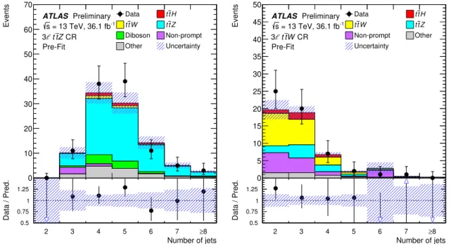
The Higgs boson signal (m H = 125 GeV) is shown as filled histograms on top of the fitted backgrounds both after the global fit (indicated as “best fit”) and as expected from the SM

In the 3-lepton analysis the total experimental uncertainty, including the 3.6% contribution from the luminosity determination, is 5% for the signal in both regions, while for

For the backgrounds normalised using CRs (WW for the N jet = 0 and N jet = 1 analyses and top in the N jet = 1 and ≥ 2 analyses), the sources of uncertainty can be grouped into

This analysis also probes the spin and parity (J P ) using the H → ZZ (∗) → 4` decay, through the observed distributions of the two Z (∗) boson masses, one production angle and

The invariant mass distributions and their composition obtained from the high-statistics simulation model based on SHERPA for the diphoton component have been cross checked against

The dashed curves show the median expected local p 0 under the hypothesis of a Standard Model Higgs boson production signal at that mass.. The horizontal dashed lines indicate

● We had already good hints where to expect the Higgs ( according to the SM ) from high precision Z-pole measurements. ● Direct searches @ LEP and @ Tevatron remained inconclusive,

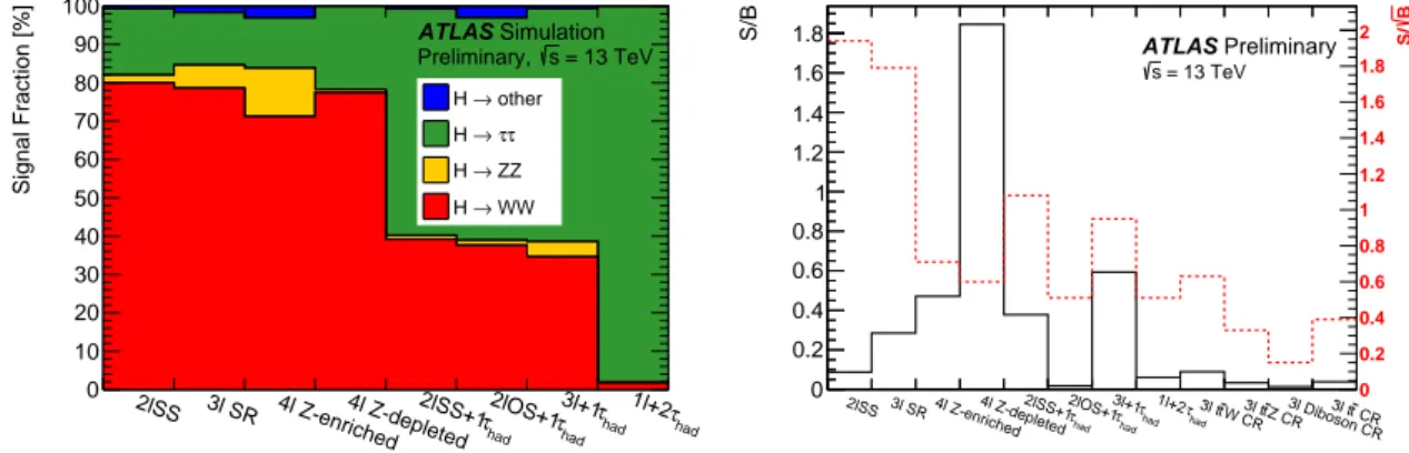
Figure 2: Left: Distribution of signal (red histogram), background (grey histogram) and data events sorted in similar signal-to-background ratio obtained from the fit to