Search for the decay of the Higgs boson to charm quarks with the ATLAS experiment

(1)

ATLAS-CONF-2017-078 07November2017

ATLAS CONF Note

ATLAS-CONF-2017-078

7th November 2017

Search for the decay of the Higgs boson to charm quarks with the ATLAS experiment

The ATLAS Collaboration

A direct search for the Standard Model Higgs boson decaying to a pair of charm quarks is presented. Associated production of the Higgs and Z bosons, in the decay mode Z H →

`

⁺

`

⁻

c c ¯ is studied. A dataset with an integrated luminosity of 36.1 fb

⁻¹

of pp collisions at

√ s = 13 TeV recorded by the ATLAS experiment at the LHC is used. The H → c c ¯ signature is identified using charm tagging algorithms. The observed (expected) upper limit on σ(pp → Z H) × B(H → c c) ¯ is 2.7 (3 . 9

⁺²−1^..¹1

) pb at the 95% confidence level for a Higgs boson mass of 125 GeV, while the Standard Model value is 25.5 fb.

Reproduction of this article or parts of it is allowed as specified in the CC-BY-4.0 license.

(2)

In July 2012, the ATLAS and CMS collaborations discovered a new particle in searches for the Standard Model (SM) Higgs boson with a mass of approximately 125 GeV [1, 2] at the Large Hadron Collider (LHC) [3]. Subsequent measurements have indicated that this particle is consistent with the SM Higgs boson [4–10], denoted by H . Direct evidence for the Yukawa coupling of the Higgs boson to the top [9]

and bottom [11, 12] quarks has recently been obtained. However, measurements of the Yukawa coupling of the Higgs boson to quarks in generations other than the third are very difficult at hadron colliders, due to small branching ratios, large backgrounds, and challenges in jet flavor identification. In this note, the first direct search by the ATLAS experiment for the decay of the Higgs boson to a pair of charm ( c ) quarks is presented. This search targets the production of the Higgs boson in association with a Z boson decaying to charged leptons: Z(`

⁺

`

⁻

)H(c c) ¯ , where ` = e, µ .

In the SM, the branching fraction for a Higgs boson with a mass of 125 GeV to decay to a pair of charm quarks is predicted to be 2.9% [13] and the inclusive cross-section for σ(pp → Z H) × B(H → c c) ¯ is 25.5 fb at

√ s = 13 TeV [14]. Rare exclusive decays of the Higgs boson to a light vector meson or quarkonium state and a photon have been proposed as a way to probe the couplings of the second generation quarks to the Higgs boson [15–18]. Previously, the ATLAS collaboration presented an indirect search for the decay of the Higgs boson to c -quarks via the decay to J/ψγ obtaining a branching ratio limit of 1 . 5 × 10

⁻³

at the 95% confidence level (CL), which approximately corresponds to a limit of 220 times the expectation from the SM [17, 19]. Bounds on Higgs boson branching ratios to unobserved final states and fits to global rates impose B(H → c c) ¯ < 20% at the 95% CL, assuming SM Higgs boson production cross-sections [20]. These limits can still accommodate large modifications to the Higgs boson coupling to charm quarks from new physics [20]. This note aims to characterize sensitivity of the ATLAS experiment to Higgs boson decays to c c ¯ and introduce this particular approach as the most promising way to study the couplings of the Higgs boson to second-generation quarks.

The search is performed using pp collision data recorded with the ATLAS detector [21] in 2015 and 2016 at

√ s = 13 TeV. The ATLAS detector at the LHC covers nearly the entire solid angle around the collision point.

¹

It consists of an inner tracking detector surrounded by a thin superconducting solenoid, electromagnetic and hadronic calorimeters, and a muon spectrometer incorporating three large superconducting toroidal magnets. For the

√ s = 13 TeV running period an additional pixel layer, the Insertable B-Layer [22] was installed. After the application of beam, detector and data quality requirements, the integrated luminosity considered corresponds to 36 . 1 ± 0 . 8 fb

⁻¹

, measured following a methodology similar to that detailed in Ref. [23]. Events are required to contain exactly two same-flavor leptons with an invariant mass consistent with that of the Z boson, and at least two jets of which one or two are required to be identified as charm jets ( c -jets) as described below. The term lepton refers to only electrons or muons in this note. The analysis procedure is validated using a measurement of the yield of ZW and Z Z production, where the sample is enriched in W → cs, cd and Z → c c ¯ decays. Further details of the analysis procedure can be found in Ref. [11].

Monte Carlo (MC) simulated samples are produced for signal and background processes using the full ATLAS detector simulation [24] based on Geant4 [25]. The MC generators used for each signal and background sample, together with the set of tuned parameters used for the modeling of the parton shower, hadronization, and underlying event, as well as the parton distribution functions (PDFs) are listed in

1ATLAS uses a right-handed coordinate system with its origin at the nominal interaction point (IP) in the center of the detector and thez-axis along the beam pipe. The x-axis points from the IP to the center of the LHC ring, and the y-axis points upwards. Cylindrical coordinates(r, φ)are used in the transverse plane, φ being the azimuthal angle around thez-axis.

The pseudorapidity is defined in terms of the polar angleθasη=−ln tan(θ/2). Angular distance is measured in units of

∆R≡p

(∆η)2+(∆φ)2.

(3)

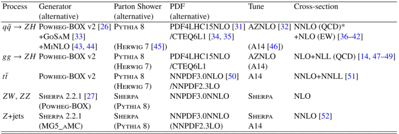
Table 1: The configurations used for event generation of the signal and background processes. If two PDFs are shown, the first is used for the matrix element calculation and the second for the parton shower, otherwise the same is used for both. Alternative generators and configurations used to estimate systematic uncertainties are indicated in parenthesis. “Tune” refers to the underlying-event tuned parameters of the parton shower generator. “MG5_aMC”

refers to MadGraph5_aMC@NLO 2.2.1 [28]; “Pythia 8” refers to version 8.212 [29]. Heavy-flavor hadron decays modeled by EvtGen 1.2.0 [30] are used for all samples except those generated using Sherpa. The precision of the cross-sections used to normalize the predictions of the event generators are indicated. Theqq¯→Z Hcross-section is estimated by subtracting thegg → Z Hcross-section from thepp→ Z Hcross-section. The asterisk (*) in the last column denotes that the indicated precision is for thepp→Z Hcross-section.

Process Generator Parton Shower PDF Tune Cross-section

(alternative) (alternative) (alternative)

qq¯→Z HPowheg-BOX v2 [26] Pythia 8 PDF4LHC15NLO [31] AZNLO [32] NNLO (QCD)*

+GoSaM [33] /CTEQ6L1 [34,35] +NLO (EW) [36–42]

+MiNLO [43,44] (Herwig 7 [45]) (A14 [46])

gg→Z HPowheg-BOX v2 Pythia 8 PDF4LHC15NLO AZNLO NLO+NLL (QCD) [14,47–49]

(Herwig 7) /CTEQ6L1 (A14)

t¯t Powheg-BOX v2 Pythia 8 NNPDF3.0NLO [50] A14 NNLO+NNLL [51]

(Herwig 7) /NNPDF2.3LO

ZW,Z Z Sherpa 2.2.1 [27] Sherpa NNPDF3.0NNLO Sherpa NLO (Powheg-BOX) (Pythia 8)

Z+jets Sherpa 2.2.1 Sherpa NNPDF3.0NNLO Sherpa NNLO [52]

(MG5_aMC) (Pythia 8) (NNPDF2.3LO) A14

Table 1. Signal events are produced at next to leading order (NLO) for the q q ¯ → Z H process and at leading order (LO) for the gg → Z H process with Powheg-BOX v2 [26]. The dominant Z +jets background and the resonant diboson ZW and Z Z processes are generated using Sherpa 2.2.1 [27]. The t¯ t background is generated using the Powheg-BOX v2 MC generator. Backgrounds from single top and multijet production as well as the contribution from Higgs decays other than b b ¯ and c c ¯ are assessed to be negligible and not considered further. The Higgs boson mass is set to m

_H

= 125 GeV and the top-quark mass is set to 172.5 GeV.

Events are required to have at least one reconstructed primary vertex. Electron candidates are reconstructed from energy clusters in the electromagnetic calorimeter that are associated with charged particle tracks reconstructed in the inner detector [53, 54]. Muon candidates are reconstructed by combining inner detector tracks with tracks in the muon spectrometer or isolated energy deposits in the calorimeters consistent with the passage of a minimum-ionising particle [55]. For data recorded in 2015, the single- electron (muon) trigger required a candidate with p

_T

> 24 ( 20 ) GeV; in 2016 the p

_T

threshold was raised to 26 GeV for both electrons and muons. Events are required to contain a pair of same flavor leptons, both satisfying p

_T

> 7 GeV and |η| < 2 . 5. At least one lepton must have p

_T

> 27 GeV and correspond to a lepton which passed the trigger. The two leptons are required to satisfy loose track-isolation criteria with an efficiency greater than 99%. They are required to have opposite charge in dimuon events, but not in dielectron events due to the non-negligible charge misidentification rate of electrons. The invariant mass of the dilepton system is required to be consistent with the mass of the Z boson: 81 GeV < m

_``

< 101 GeV.

Jets are reconstructed from topological energy clusters in the calorimeters [56, 57] using the anti- k

_t

algorithm [58] with a radius parameter of 0.4. The jet energy is corrected using a jet-area based

technique [59, 60] and calibrated [61, 62] using p

_T

and η -dependent correction factors determined

from simulation, with residual corrections from internal jet properties. Further corrections from in situ

(4)

jet rejection b

10

light jet rejection

10 102

103

104

jet efficiencyc

0.1 0.15 0.2 0.25 0.3 0.35 0.4 0.45 0.5 ATLAS Simulation Preliminary

t = 13 TeV, t

s c efficiency 41%

efficiency 30%

c efficiency 20%

c

41% efficiency WP

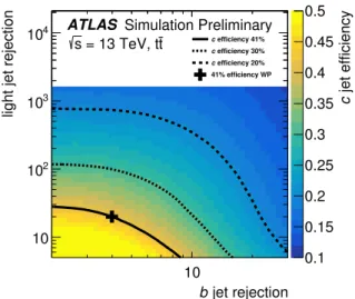
Figure 1: Thec-jet tagging efficiency (coloured scale) as a function of theb-jet (x-axis) andl-jet (y-axis) rejection as obtained from simulatedtt¯events. The cross denotes the choice of the selection criterion used in this analysis.

The solid and dotted black lines indicate the contours in the rejection space for the fixedc-tagging efficiency of the criterion used in this analysis and two alternative fixedc-tagging efficiency criteria respectively.

measurements are applied to data. Selected jets must have p

_T

> 20 GeV and |η| < 2 . 5. Events are required to contain at least two jets. If a muon is found within a jet, its momentum is added to the selected jet. An overlap removal procedure is applied to resolve cases in which the same physical object is reconstructed multiple times, e.g. an electron also reconstructed as a jet.

In simulated events, jets are labelled according to the presence of a heavy-flavor hadron with p

_T

> 5 GeV within a cone around the jet axis of size ∆R = 0 . 3. If a b -hadron is found the jet is labelled as a b -jet.

If no b -hadron is found, but a c -hadron is present, then the jet is labelled as a c -jet. Otherwise the jet is labelled as a light flavor ( u, d, s quarks and gluon) jet ( l -jet).

Flavor tagging algorithms exploit the different lifetimes of b , c and light flavor hadrons. A c -tagging algorithm is used to identify c -jets. These jets are particularly challenging to tag with high efficiency because c -hadrons have shorter lifetimes and decay to a lower number of charged particles than b -hadrons.

Two multivariate discriminants are trained: the first separates c -jets from l -jets, while the second separates c -jets from b -jets. The inputs to these discriminants are the same variables used for b -tagging [63, 64].

Selection criteria are applied in the two-dimensional multivariate discriminant space as shown in Fig. 1, to obtain an efficiency of 41% for c -jets and rejection factors (inverse efficiencies) of 4 and 20 for b -jets and l -jets respectively. The efficiencies are calibrated to data using b -quarks from t → W b and c -quarks from W → cs, cd with identical methods to those used for b -tagging algorithms [63]. To reduce statistical uncertainties in the simulation, rather than imposing a direct requirement on the c -tagging discriminants, the events are weighted according to the tagging efficiencies of their jets, parameterized as a function of jet flavor, p

_T

, η and the angular separation between jets.

Data are analyzed in four categories with different expected signal purities. The invariant mass of the dijet system, m

_c_c_¯

, constructed using the two highest p

_T

jets, is the discriminating variable in each category. These categories are defined based on the transverse momentum of the reconstructed Z boson, p

^Z

T

(75 GeV < p

^Z

T

< 150 GeV and p

^Z

T

> 150 GeV) and the number of c -tags amongst the leading jets (either one or two). The lower requirement on p

^Z

T

exploits the harder p

^Z

T

distribution in Z H production

(5)

than in the main Z + jets background. To reject background events, the angular separation between the two jets constituting the dijet system, ∆R

_c_c_¯

, is required to be less than 2.2. This requirement is tightened to 1.5 (1.3) for events satisfying 150 < p

^Z

T

< 200 GeV ( p

^Z

T

> 200 GeV). The signal acceptance ranges from 0.5% to 3.4% depending on the category. A joint binned maximum profile likelihood fit to m

_c_c_¯

in the four categories is used to extract the signal yield and estimate the normalization of the Z +jets background. The fit is performed using 15 uniform width bins in each category in the range of 50 GeV < m

_c_c_¯

< 200 GeV.

The parameter of interest, µ , common to all categories, is the signal strength, defined as the ratio of the measured signal yield to the prediction from the SM.

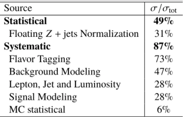
Systematic uncertainties affecting the signal and background predictions include theoretical uncertainties in the signal and background modeling and experimental uncertainties. They are summarized in Table 2, which shows their relative impact on the fitted value of µ . Uncertainties in the m

_c_c_¯

shape of the simulated backgrounds are assessed by comparisons between nominal and alternative MC generators as indicated in Table 1.

The systematic uncertainties are incorporated within the statistical model through nuisance parameters that modify the shape and/or normalization of the expected distributions. The statistical model includes additional terms which parametrize the constraints from auxiliary measurements on the uncertainties of these parameters. The effects of statistical uncertainties in the simulation samples are accounted for by the statistical model. The Z +jets background is normalised from the data through the inclusion of an unconstrained normalization parameter for each analysis category. The normalization parameters range between 1.13 and 1.30. All other background normalization factors are correlated between categories with acceptance uncertainties typically of the order of 10% to account for relative variations between categories.

The dominant contributions to the uncertainty in µ are the efficiency of the tagging algorithms, the jet energy scale and resolution, and the modeling of the backgrounds. The largest uncertainty is due to the normalization of the Z +jets background. The typical size of the relative uncertainty on the tagging efficiency is 20% for c -jets, 5% for b -jets, and 20% for l -jets.

Source σ/σ

_tot

Statistical 49%

Floating Z + jets Normalization 31%

Systematic 87%

Flavor Tagging 73%

Background Modeling 47%

Lepton, Jet and Luminosity 28%

Signal Modeling 28%

MC statistical 6%

Table 2: Breakdown of the relative contributions to the total uncertainty inµ. The statistical uncertainty includes the contribution from the floating Z+jets normalization parameters, the contribution from which is also shown separately. The total systematic uncertainty and its components are shown. The sum in quadrature of the individual components differs from the total uncertainty due to correlations between the components.

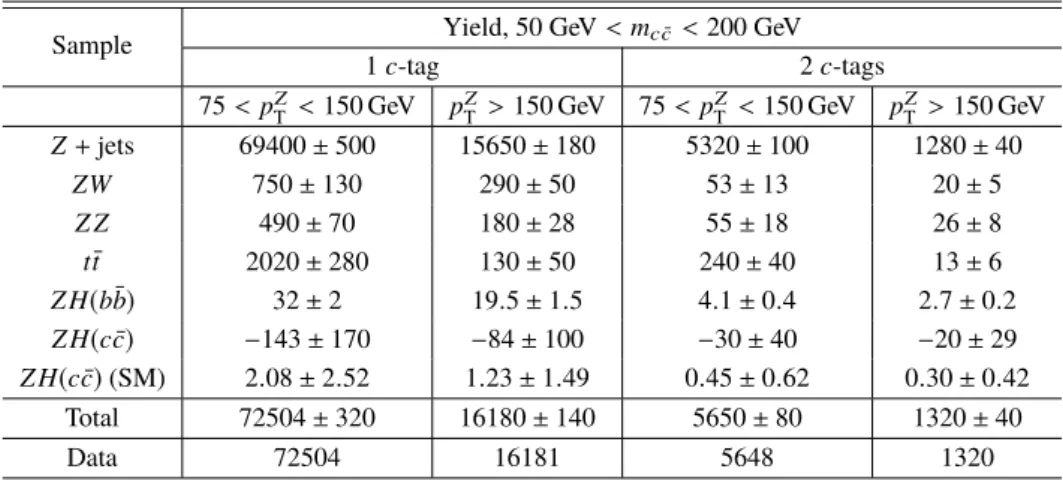
The fitted signal and background yields are listed in Table 3. The most significant background source is

Z +jets production. The m

_c_c_¯

distributions in all signal categories are shown in Fig. 2 with the background

(6)

Sample Yield, 50 GeV<m_c_c_¯ <200 GeV

1c-tag 2c-tags

75<p^Z

T <150 GeV p^Z

T >150 GeV 75<p^Z

T <150 GeV p^Z

T >150 GeV Z+jets 69400±500 15650±180 5320±100 1280±40

ZW 750±130 290±50 53±13 20±5

Z Z 490±70 180±28 55±18 26±8

tt¯ 2020±280 130±50 240±40 13±6

Z H(b¯b) 32±2 19.5±1.5 4.1±0.4 2.7±0.2 Z H(cc)¯ −143±170 −84±100 −30±40 −20±29 Z H(cc¯)(SM) 2.08±2.52 1.23±1.49 0.45±0.62 0.30±0.42

Total 72504±320 16180±140 5650±80 1320±40

Data 72504 16181 5648 1320

Table 3: The post-fit yields for the signal and the post-fit yields for the background processes in each signal region from the profile likelihood fit. The uncertainties include both statistical and systematic contributions. The post-fit Z H(cc)¯ signal yields and associated uncertainties, scaled to the SM expectation (µ=1), are also indicated.

shapes and normalizations according to the result of the fit. The background normalization has been corrected and good agreement is observed between the post-fit shapes of the distributions and the data.

The analysis procedure is validated by measuring the yield of ZV production, where V is taken to indicate W or Z , in the same final states and with the same event selection. The fraction of the Z Z yield that comes from Z → c c ¯ decays is ∼ 55% (20%) in the 2 c -tag (1 c -tag) categories, while the fraction of the ZW yield from W → cs, cd is ∼ 65% for both the 2 and 1 c -tag categories. The contribution of the Higgs boson decay to c c ¯ and b b ¯ is treated as a background and constrained to the expectation from the SM within its theoretical uncertainty. The diboson signal strength is measured to be µ

_ZV

= 0 . 6

⁺⁰₋₀^._.⁵₄

and has an observed (expected) significance of 1.4 (2 . 2) standard deviations.

The best fit value for the Z H(c c) ¯ signal strength is µ

Z H

= − 69 ± 101. By assuming a signal with the kinematics of the SM Higgs boson, model-dependent corrections are made when extrapolating to the inclusive phase space. Hence, an upper limit on σ(pp → Z H) × B(H → c c) ¯ is computed using a modified frequentist CL

s

method [65, 66] with the profile likelihood ratio as the test statistic. The observed upper limit is found to be 2.7 pb at the 95% CL. The expected upper limit is 3 . 9

⁺²₋₁^._.¹₁

pb at the 95% CL. This corresponds to an observed (expected) upper limit on µ at the 95% CL of 110 (150

⁺⁸⁰₋₄₀

). The uncertainties on the expected limits correspond to the ± 1 σ interval of background-only pseudo-experiments. The result depends weakly on the assumption of SM H → b b ¯ . The change in the observed limit remains within 5%

of the nominal value when the assumed value for normalization of the Z H(b b) ¯ background is varied from

zero to twice the SM expectation.

(7)

obs_x_Chan_mi_1t2pj_2L 60 80 100 120 140 160 180 200

Events / ( 10 )

0 2 4 6 8 10

103

×

60 80 100 120 140 160 180 200

Events / 10 GeV

10 102

103

104

105

106 ATLAS Preliminary = 13 TeV, 36.1 fb-1 s

< 150 GeV Z pT -tag, 75 <

1 c

Data Pre-fit Fit Result Z + jets

t t ZZ ZW

) b ZH(b

SM) ) (100× c ZH(c

[GeV]

c

mc

60 80 100 120 140 160 180 200

Data/Bkgd.

0.9 1.0 1.1

(a) 1c-tag 75<p^Z

T <150 GeV

obs_x_Chan_hi_1t2pj_2L 60 80 100 120 140 160 180 200

Events / ( 10 )

0 0.5 1 1.5 2 2.5

103

×

60 80 100 120 140 160 180 200

Events / 10 GeV

10 102

103

104

105

ATLAS Preliminary = 13 TeV, 36.1 fb-1 s

> 150 GeV Z pT -tag, 1 c

t t ZZ ZW

) b ZH(b

SM) ) (100× c ZH(c

[GeV]

c

mc

60 80 100 120 140 160 180 200

Data/Bkgd.

0.9 1.0 1.1

(b) 1c-tagp^Z

T >150 GeV

obs_x_Chan_mi_2t2pj_2L 60 80 100 120 140 160 180 200

Events / ( 10 )

0 100 200 300 400 500 600 700 800

60 80 100 120 140 160 180 200

Events / 10 GeV

1 10 102

103

104

105

< 150 GeV Z pT -tags, 75 <

2 c

t t ZZ ZW

) b ZH(b

×SM) ) (100 c ZH(c

[GeV]

c

mc

60 80 100 120 140 160 180 200

Data/Bkgd.

0.80.9 1.01.1 1.2

(c) 2c-tags 75<p^Z

T <150 GeV

obs_x_Chan_hi_2t2pj_2L 60 80 100 120 140 160 180 200

Events / ( 10 )

0 20 40 60 80 100 120 140 160 180 200 220

60 80 100 120 140 160 180 200

Events / 10 GeV

1 10 102

103

104 ATLAS Preliminary = 13 TeV, 36.1 fb-1 s

> 150 GeV Z pT -tags, 2 c

t t ZZ ZW

) b ZH(b

×SM) ) (100 c ZH(c

[GeV]

c

mc

60 80 100 120 140 160 180 200 Data/Bkgd. 0.60.81.01.21.4

(d) 2c-tagsp^Z

T >150 GeV

Figure 2: Observed and predictedm_c_c_¯distributions in the four analysis categories. The expected signal (pre-fit) is scaled by a factor of 100. The backgrounds are shown corrected to the results of the fit to the data. The predicted background from the simulation is shown as red dashed histograms. The ratios of the data to the fitted background are shown in the lower panels. The error bands indicate the quadratic sum of the statistical and systematic uncertainties in the background prediction. Arrows denote where the central value of a data point lies above or below the visible range.

To conclude, a search for the decay of the Higgs boson to charm quarks has been performed using 36.1 fb

⁻¹

of data collected with the ATLAS detector in pp collisions at

√ s = 13 TeV at the LHC. No significant

excess of Z H(c c) ¯ production is observed with respect to the SM background expectation. The observed

upper limit on σ(pp → Z H) × B(H → c c) ¯ is 2.7 pb at the 95% C.L. The corresponding expected upper

limit is 3 . 9

⁺²₋₁^._.¹₁

pb. This is the most stringent limit to date in direct searches for the decay of the Higgs

boson to charm quarks.

(8)

References

[1] ATLAS Collaboration, Observation of a new particle in the search for the Standard Model Higgs boson with the ATLAS detector at the LHC , Phys. Lett. B 716 (2012) p. 1,

arXiv: 1207.7214 [hep-ex] . [2] CMS Collaboration,

Observation of a new boson with mass near 125 GeV in pp collisions at √

s = 7 and 8 TeV , JHEP 06 (2013) p. 081, arXiv: 1303.4571 [hep-ex] .

[3] L. Evans and P. Bryant, LHC Machine , JINST 3 (2008) S08001.

[4] ATLAS Collaboration, Measurements of the Higgs boson production and decay rates and coupling strengths using pp collision data at √

s = 7 and 8 TeV in the ATLAS experiment , Eur. Phys. J. C76 (2016) p. 6, arXiv: 1507.04548 [hep-ex] .

[5] CMS Collaboration,

Precise determination of the mass of the Higgs boson and tests of compatibility of its couplings with the standard model predictions using proton collisions at 7 and 8 TeV ,

Eur. Phys. J. C 75 (2015) p. 212, arXiv: 1412.8662 [hep-ex] . [6] CMS Collaboration,

Study of the Mass and Spin-Parity of the Higgs Boson Candidate Via Its Decays to Z Boson Pairs , Phys. Rev. Lett. 110 (2013) p. 081803, arXiv: 1212.6639 [hep-ex] .

[7] ATLAS Collaboration, Evidence for the spin-0 nature of the Higgs boson using ATLAS data , Phys. Lett. B 726 (2013) p. 120, arXiv: 1307.1432 [hep-ex] .

[8] CMS Collaboration, Constraints on the spin-parity and anomalous HVV couplings of the Higgs boson in proton collisions at 7 and 8 TeV , Phys. Rev. D 92 (2015) p. 012004,

arXiv: 1411.3441 [hep-ex] . [9] ATLAS and CMS Collaborations,

Measurements of the Higgs boson production and decay rates and constraints on its couplings from a combined ATLAS and CMS analysis of the LHC pp collision data at √

s = 7 and 8 TeV , JHEP 08 (2016) p. 045, arXiv: 1606.02266 [hep-ex] .

[10] ATLAS and CMS Collaborations, Combined Measurement of the Higgs Boson Mass in pp Collisions at √

s = 7 and 8 TeV with the ATLAS and CMS Experiments , Phys. Rev. Lett. 114 (2015) p. 191803, arXiv: 1503.07589 [hep-ex] .

[11] ATLAS Collaboration, Evidence for the H → b b ¯ decay with the ATLAS detector , (2017), arXiv: 1708.03299 [hep-ex] .

[12] CMS Collaboration, Evidence for the Higgs boson decay to a bottom quark-antiquark pair , (2017), arXiv: 1709.07497 [hep-ex] .

[13] A. Djouadi, J. Kalinowski and M. Spira, HDECAY: A program for Higgs boson decays in the Standard Model and its supersymmetric extension , Comput. Phys. Commun. 108 (1998) p. 56, arXiv: hep-ph/9704448 [hep-ph] .

[14] D. de Florian et al.,

Handbook of LHC Higgs Cross Sections: 4. Deciphering the Nature of the Higgs Sector , (2016),

arXiv: 1610.07922 [hep-ph] .

(9)

[15] G. T. Bodwin, F. Petriello, S. Stoynev and M. Velasco,

Higgs boson decays to quarkonia and the H cc ¯ coupling , Phys. Rev. D88 (2013) p. 053003, arXiv: 1306.5770 [hep-ph] .

[16] A. L. Kagan et al., Exclusive Window onto Higgs Yukawa Couplings , Phys. Rev. Lett. 114 (2015) p. 101802, arXiv: 1406.1722 [hep-ph] . [17] ATLAS Collaboration,

Search for Higgs and Z Boson Decays to J/ψγ and Υ(nS)γ with the ATLAS Detector , Phys. Rev. Lett. 114 (2015) p. 121801, arXiv: 1501.03276 [hep-ex] .

[18] ATLAS Collaboration, Search for Higgs and Z Boson Decays to φ γ with the ATLAS Detector , Phys. Rev. Lett. 117 (2016) p. 111802, arXiv: 1607.03400 [hep-ex] .

[19] G. Perez, Y. Soreq, E. Stamou and K. Tobioka,

Constraining the charm Yukawa and Higgs-quark coupling universality , Phys. Rev. D92 (2015) p. 033016, arXiv: 1503.00290 [hep-ph] .

[20] C. Delaunay, T. Golling, G. Perez and Y. Soreq, Enhanced Higgs boson coupling to charm pairs , Phys. Rev. D89 (2014) p. 033014, arXiv: 1310.7029 [hep-ph] .

[21] ATLAS Collaboration, The ATLAS Experiment at the CERN Large Hadron Collider , JINST 3 (2008) S08003.

[22] ATLAS Collaboration, ATLAS Insertable B-Layer Technical Design Report , CERN-LHCC-2010-013. ATLAS-TDR-19, 2010,

url: http://cds.cern.ch/record/1291633 . [23] ATLAS Collaboration,

Luminosity determination in pp collisions at √

s = 8 TeV using the ATLAS detector at the LHC , Eur. Phys. J. C 76 (2016) p. 653, arXiv: 1608.03953 [hep-ex] .

[24] ATLAS Collaboration, The ATLAS Simulation Infrastructure , Eur. Phys. J. C 70 (2010) p. 823, arXiv: 1005.4568 [hep-ex] .

[25] GEANT4 Collaboration, S. Agostinelli et al., GEANT4 - A Simulation toolkit , Nucl. Instrum. Meth. A 506 (2003) p. 250.

[26] S. Alioli, P. Nason, C. Oleari and E. Re, A general framework for implementing NLO calculations in shower Monte Carlo programs: the POWHEG BOX , JHEP 06 (2010) p. 043,

arXiv: 1002.2581 [hep-ph] .

[27] T. Gleisberg et al., Event generation with SHERPA 1.1 , JHEP 0902 (2009) p. 007, arXiv: 0811.4622 [hep-ph] .

[28] J. Alwall et al., The automated computation of tree-level and next-to-leading order differential cross sections, and their matching to parton shower simulations , JHEP 07 (2014) p. 079, arXiv: 1405.0301 [hep-ph] .

[29] T. Sjöstrand, S. Mrenna and P. Z. Skands, A brief introduction to PYTHIA 8.1 , Comput. Phys. Commun. 178 (2008) p. 852, arXiv: 0710.3820 [hep-ph] . [30] D. J. Lange, The EvtGen particle decay simulation package ,

Nucl. Instrum. Meth. Phys. Res. A 462 (2001) p. 152.

[31] J. Butterworth et al., PDF4LHC recommendations for LHC Run II ,

J. Phys. G43 (2016) p. 023001, arXiv: 1510.03865 [hep-ph] .

(10)

[32] ATLAS Collaboration, Measurement of the Z/γ

^∗

boson transverse momentum distribution in pp collisions at √

s = 7 TeV with the ATLAS detector , JHEP 2014 (2014) p. 55, arXiv: 1406.3660 [hep-ex] .

[33] G. Cullen et al., Automated one-loop calculations with GoSam , Eur. Phys. J. C72 (2012) p. 1889, arXiv: 1111.2034 [hep-ph] .

[34] J. Pumplin et al.,

New generation of parton distributions with uncertainties from global QCD analysis , JHEP 07 (2002) p. 012, arXiv: hep-ph/0201195 [hep-ph] .

[35] P. M. Nadolsky, H.-L. Lai, Q.-H. Cao, J. Huston, J. Pumplin et al.,

Implications of CTEQ global analysis for collider observables , Phys. Rev. D 78 (2008) p. 013004, arXiv: 0802.0007 [hep-ph] .

[36] M. Ciccolini, S. Dittmaier and M. Krämer,

Electroweak radiative corrections to associated W H and Z H production at hadron colliders , Phys. Rev. D68 (2003) p. 073003, arXiv: hep-ph/0306234 [hep-ph] .

[37] O. Brein, A. Djouadi and R. Harlander,

NNLO QCD corrections to the Higgs-strahlung processes at hadron colliders , Phys. Lett. B579 (2004) p. 149, arXiv: hep-ph/0307206 [hep-ph] .

[38] G. Ferrera, M. Grazzini and F. Tramontano,

Associated W H production at hadron colliders: a fully exclusive QCD calculation at NNLO , Phys. Rev. Lett. 107 (2011) p. 152003, arXiv: 1107.1164 [hep-ph] .

[39] O. Brein, R. Harlander, M. Wiesemann and T. Zirke,

Top-quark mediated effects in hadronic Higgs-Strahlung , Eur. Phys. J. C72 (2012) p. 1868, arXiv: 1111.0761 [hep-ph] .

[40] G. Ferrera, M. Grazzini and F. Tramontano,

Higher-order QCD effects for associated WH production and decay at the LHC , JHEP 04 (2014) p. 039, arXiv: 1312.1669 [hep-ph] .

[41] G. Ferrera, M. Grazzini and F. Tramontano,

Associated ZH production at hadron colliders: the fully differential NNLO QCD calculation , Phys. Lett. B740 (2015) p. 51, arXiv: 1407.4747 [hep-ph] .

[42] J. M. Campbell, R. K. Ellis and C. Williams, Associated production of a Higgs boson at NNLO , JHEP 06 (2016) p. 179, arXiv: 1601.00658 [hep-ph] .

[43] K. Hamilton, P. Nason and G. Zanderighi, MINLO: multi-scale improved NLO , JHEP 10 (2012) p. 155, arXiv: 1206.3572 [hep-ph] .

[44] G. Luisoni, P. Nason, C. Oleari and F. Tramontano, HW

^±

/HZ + 0 and 1 jet at NLO with the POWHEG BOX interfaced to GoSam and their merging within MiNLO , JHEP 10 (2013) p. 083, arXiv: 1306.2542 [hep-ph] .

[45] J. Bellm et al., Herwig 7.0/Herwig++ 3.0 release note , Eur. Phys. J. C76 (2016) p. 196, arXiv: 1512.01178 [hep-ph] .

[46] ATLAS Collaboration, ATLAS Pythia 8 tunes to 7 TeV data , ATL-PHYS-PUB-2014-021, 2014, url: https://cds.cern.ch/record/1966419 .

[47] L. Altenkamp, S. Dittmaier, R. V. Harlander, H. Rzehak and T. J. E. Zirke,

Gluon-induced Higgs-strahlung at next-to-leading order QCD , JHEP 02 (2013) p. 078,

arXiv: 1211.5015 [hep-ph] .

(11)

[48] B. Hespel, F. Maltoni and E. Vryonidou,

Higgs and Z boson associated production via gluon fusion in the SM and the 2HDM , JHEP 06 (2015) p. 065, arXiv: 1503.01656 [hep-ph] .

[49] L. Altenkamp, S. Dittmaier, R. V. Harlander, H. Rzehak and T. J. Zirke,

Gluon-induced Higgs-strahlung at next-to-leading order QCD , JHEP 02 (2013) p. 078, arXiv: 1211.5015 [hep-ph] .

[50] R. D. Ball et al., Parton distributions with LHC data , Nucl. Phys. B 867 (2013) p. 244, arXiv: 1207.1303 [hep-ph] .

[51] M. Czakon and A. Mitov,

Top++: A program for the calculation of the top-pair cross-Section at hadron colliders , Comput. Phys. Commun. 185 (2014) p. 2930, arXiv: 1112.5675 [hep-ph] .

[52] S. Catani, L. Cieri, G. Ferrera, D. de Florian and M. Grazzini, Vector Boson Production at Hadron Colliders: A Fully Exclusive QCD Calculation at Next-to-Next-to-Leading Order ,

Phys. Rev. Lett. 103 (2009) p. 082001, arXiv: 0903.2120 [hep-ph] .

[53] ATLAS Collaboration, Electron efficiency measurements with the ATLAS detector using 2012 LHC proton-proton collision data , Eur. Phys. J. C77 (2017) p. 195,

arXiv: 1612.01456 [hep-ex] .

[54] ATLAS Collaboration, Electron efficiency measurements with the ATLAS detector using the 2015 LHC proton–proton collision data , ATLAS-CONF-2016-024, 2016,

url: https://cds.cern.ch/record/2157687 .

[55] ATLAS Collaboration, Muon reconstruction performance of the ATLAS detector in proton–proton collision data at √

s = 13 TeV , Eur. Phys. J. C 76 (2016) p. 292, arXiv: 1603.05598 [hep-ex] . [56] ATLAS Collaboration,

Topological cell clustering in the ATLAS calorimeters and its performance in LHC Run 1 , Eur. Phys. J. C 77 (2017) p. 490, arXiv: 1603.02934 [hep-ex] .

[57] ATLAS Collaboration, Properties of jets and inputs to jet reconstruction and calibration with the ATLAS detector using proton–proton collisions at √

s = 13 TeV , ATL-PHYS-PUB-2015-036, 2015, url: https://cds.cern.ch/record/2044564 .

[58] M. Cacciari, G. P. Salam and G. Soyez, The anti-k

_t

jet clustering algorithm , JHEP 04 (2008) p. 063, arXiv: 0802.1189 [hep-ph] .

[59] M. Cacciari and G. P. Salam, Pileup subtraction using jet areas , Phys. Lett. B 659 (2008) p. 119, arXiv: 0707.1378 [hep-ph] .

[60] ATLAS Collaboration, Performance of pile-up mitigation techniques for jets in pp collisions at

√ s = 8 TeV using the ATLAS detector , Eur. Phys. J. C 76 (2016) p. 581, arXiv: 1510.03823 [hep-ex] .

[61] ATLAS Collaboration,

Jet energy measurement with the ATLAS detector in proton–proton collisions at √

s = 7 TeV , Eur. Phys. J. C 73 (2013) p. 2304, arXiv: 1112.6426 [hep-ex] .

[62] ATLAS Collaboration, Jet energy scale measurements and their systematic uncertainties in proton–proton collisions at √

s = 13 TeV with the ATLAS detector ,

Phys. Rev. D96 (2017) p. 072002, arXiv: 1703.09665 [hep-ex] .

(12)

[63] ATLAS Collaboration, Performance of b-jet identification in the ATLAS experiment , JINST 11 (2016) P04008, arXiv: 1512.01094 [hep-ex] .

[64] ATLAS Collaboration, Optimisation of the ATLAS b-tagging performance for the 2016 LHC Run , ATL-PHYS-PUB-2016-012, 2016, url: https://cds.cern.ch/record/2160731 .

[65] G. Cowan, K. Cranmer, E. Gross and O. Vitells,

Asymptotic formulae for likelihood-based tests of new physics ,

Eur. Phys. J. C 71 (2011) p. 1554, [Erratum: Eur. Phys. J. C 73 (2013) 2501], arXiv: 1007.1727 [physics.data-an] .

[66] A. L. Read, Presentation of search results: The C L

_S

technique , J. Phys. G28 (2002) p. 2693.

(13)

Appendix

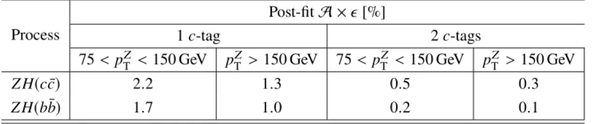
This Appendix includes a collection of supplementary figures and tabulated information. The post-fit product of the acceptance and efficiency, A × , is shown for the Z H(c c) ¯ signal and the Z H(b b) ¯ background in each category in Table 4. Figure 3 shows the m

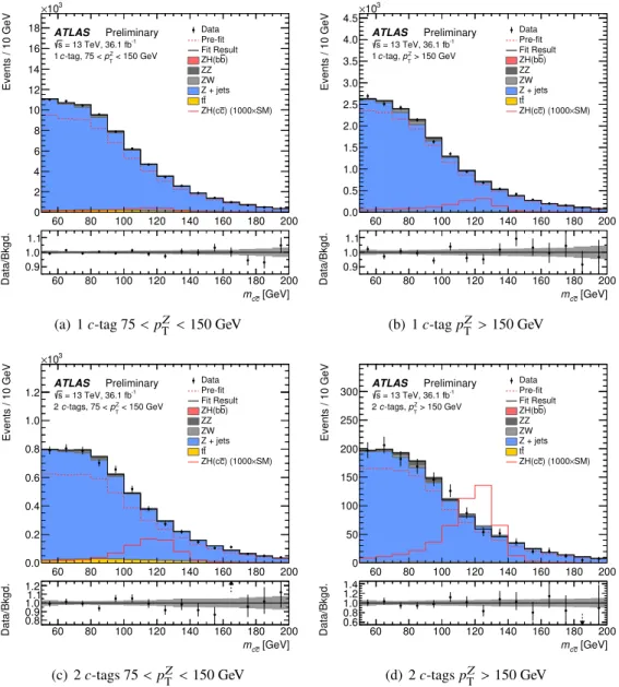
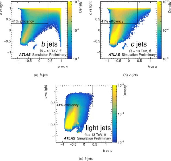
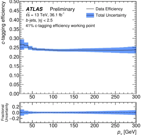
_c_c_¯

distributions corresponding to the result of the fit as shown in Figure 2 with a linear y-axis scale. The two dimensional distributions of the two c -tagging discriminants are shown in Figure 4, while Figures 5 to 7 show the calibrated efficiency of the c -tagging working point for light, c - and b -jets. The flavour composition of the Z + jets and Z (Z /W) backgrounds is shown in Figure 8 and Figure 9, respectively. The p

^Z

T

, ∆R

_{j j}

and leading (sub-leading) jet p

_T

distributions observed in data, compared to the inclusive background simulation normalised to data, are shown in Figures 10 to 13.

Process

Post-fit A × [%]

1 c -tag 2 c -tags

75 < p

^Z

T

< 150 GeV p

^Z

T

> 150 GeV 75 < p

^Z

T

< 150 GeV p

^Z

T

> 150 GeV

Z H(c c) ¯ 2 . 2 1 . 3 0 . 5 0 . 3

Z H(b b) ¯ 1 . 7 1 . 0 0 . 2 0 . 1

Table 4: The post-fit product of the acceptance and efficiency, A ×, for the Z H(cc)¯ signal and the Z H(bb)¯ background consideringZ →e⁺e⁻,Z →µ⁺µ⁻andZ →τ⁺τ⁻decays .

(14)

obs_x_Chan_mi_1t2pj_2L 60 80 100 120 140 160 180 200

Events / ( 10 )

0 2 4 6 8 10

103

×

60 80 100 120 140 160 180 200

Events / 10 GeV

0 2 4 6 8 10 12 14 16 18

103

×

< 150 GeV Z pT -tag, 75 <

1 c

Data Pre-fit Fit Result

) b ZH(b ZZ ZW Z + jets

t t

×SM) ) (1000 c ZH(c

[GeV]

c

mc

60 80 100 120 140 160 180 200

Data/Bkgd.

0.9 1.0 1.1

(a) 1c-tag 75<p^Z

T <150 GeV

obs_x_Chan_hi_1t2pj_2L 60 80 100 120 140 160 180 200

Events / ( 10 )

0 0.5 1 1.5 2 2.5

103

×

60 80 100 120 140 160 180 200

Events / 10 GeV

0.0 0.5 1.0 1.5 2.0 2.5 3.0 3.5 4.0 4.5

103

×

> 150 GeV Z pT -tag, 1 c

t t

×SM) ) (1000 c ZH(c

[GeV]

c

mc

60 80 100 120 140 160 180 200

Data/Bkgd.

0.9 1.0 1.1

(b) 1c-tagp^Z

T >150 GeV

obs_x_Chan_mi_2t2pj_2L 60 80 100 120 140 160 180 200

Events / ( 10 )

0 100 200 300 400 500 600 700 800

60 80 100 120 140 160 180 200

Events / 10 GeV

0.0 0.2 0.4 0.6 0.8 1.0 1.2

103

×

< 150 GeV Z pT -tags, 75 <

2 c

t t

×SM) ) (1000 c ZH(c

[GeV]

c

mc

60 80 100 120 140 160 180 200

Data/Bkgd.

0.80.9 1.01.1 1.2

(c) 2c-tags 75<p^Z

T <150 GeV

obs_x_Chan_hi_2t2pj_2L 60 80 100 120 140 160 180 200

Events / ( 10 )

0 20 40 60 80 100 120 140 160 180 200 220

60 80 100 120 140 160 180 200

Events / 10 GeV

0 50 100 150 200 250 300

> 150 GeV Z pT -tags, 2 c

t t

×SM) ) (1000 c ZH(c

[GeV]

c

mc

60 80 100 120 140 160 180 200

Data/Bkgd.

0.60.8 1.0 1.21.4

(d) 2c-tagsp^Z

T >150 GeV

Figure 3: Observed and predictedmcc¯distributions in the four analysis categories shown with a linear scale. The expected signal (pre-fit) is scaled by a factor of 1000. The backgrounds are shown corrected to the results of the fit to the data. The predicted background from the simulation is shown as red dashed histograms. The ratios of the data to the results of the fit are shown in the lower panel. The error bands indicate the quadratic sum of the statistical and systematic uncertainties in the background prediction. Arrows denote where the central value of a data point lies above or below the visible range.

(15)

1

− −0.5 0 0.5 1 vs c b 1

− 0.5

− 0 0.5 1

vs lightc

5

10− 4

10− 3

10−

Density

jets b

ATLAS Simulation Preliminary t = 13 TeV, t s

41% efficiency

(a)b-jets

1

− −0.5 0 0.5 1 vs c b 1

− 0.5

− 0 0.5 1

vs lightc

5

10− 4

10− 3

10−

Density

jets c

41% efficiency

(b)c-jets

1

− −0.5 0 0.5 1 vs c b 1

− 0.5

− 0 0.5 1

vs lightc

5

10− 4

10− 3

10−

Density

light jets

41% efficiency

(c)l-jets

Figure 4: The two dimensional distribution of the two multivariate discriminants trained to separatec-jets from eitherb-jets orl-jets, forb-jets,c-jets andl-jets. The selection requirement of the 41% efficiencyc-tagging working point is also shown.

(16)

50 100 150 200 250 300

-tagging efficiency c

0.00 0.05 0.10 0.15 0.20 0.25 0.30 0.35 0.40 0.45 0.50

ATLAS Preliminary

= 13 TeV, 36.1 fb-1

s

| < 2.5 -jets, |η b

41% c-tagging efficiency working point

Data Efficiency Total Uncertainty

[GeV]

p

T

50 100 150 200 250 300

Uncertainty Fractional

0.2 −

0.0 0.2

Figure 5: Thec-tagging efficiency of the 41% efficiencyc-tagging working point in data forb-jets as a function of jet transverse momentum. The uncertainty band represents the total uncertainty associated with the calibration of c-tagging efficiency in data.

(17)

50 100 150 200 250 300

-tagging efficiency c

0.0 0.1 0.2 0.3 0.4 0.5 0.6 0.7 0.8 0.9 1.0

ATLAS Preliminary

= 13 TeV, 36.1 fb-1

s

| < 2.5 -jets, |η c

[GeV]

p

T

50 100 150 200 250 300

0.2 −

0.0 0.2

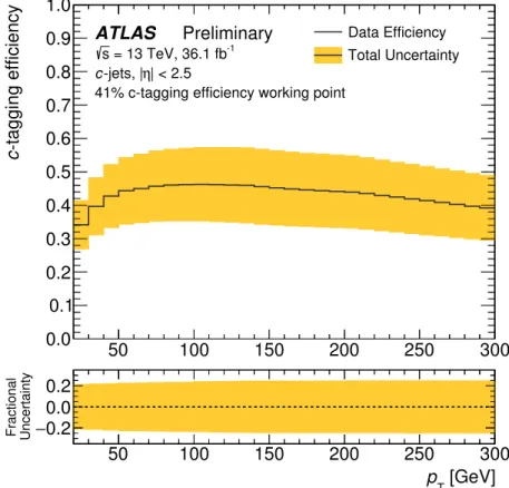
Figure 6: Thec-tagging efficiency of the 41% efficiencyc-tagging working point in data forc-jets as a function of jet transverse momentum. The uncertainty band represents the total uncertainty associated with the calibration of c-tagging efficiency in data.

(18)

50 100 150 200 250 300

-tagging efficiency c

0.00 0.05 0.10 0.15 0.20 0.25 0.30

ATLAS Preliminary

= 13 TeV, 36.1 fb-1

s

| < 2.5 light-jets, |η

[GeV]

p

T

50 100 150 200 250 300

0.2 −

0.0 0.2

Figure 7: Thec-tagging efficiency of the 41% efficiencyc-tagging working point in data for light-jets as a function of jet transverse momentum. The uncertainty band represents the total uncertainty associated with the calibration ofc-tagging efficiency in data.

(19)

[GeV]

c

mc

60 80 100 120 140 160 180 200

Events / 10 GeV

0 2 4 6 8 10 12 14 16

103

×

Z + jets Simulation Dijet Flavour Composition

ll cl cc

bl bc bb

ATLASPreliminary = 13 TeV, 36.1 fb-1 s

< 150 GeV Z pT -tag, 75 <

c 1

(a) 1c-tag 75<p^Z

T <150 GeV

[GeV]

c

mc

60 80 100 120 140 160 180 200

Events / 10 GeV

0.0 0.5 1.0 1.5 2.0 2.5 3.0 3.5 4.0

103

×

ll cl cc

bl bc bb

> 150 GeV Z pT -tag, c 1

(b) 1c-tagp^Z

T >150 GeV

[GeV]

c

mc

60 80 100 120 140 160 180 200

Events / 10 GeV

0.0 0.2 0.4 0.6 0.8 1.0

103

×

ll cl cc

bl bc bb

< 150 GeV Z pT -tags, 75 <

c 2

(c) 2c-tags 75<p^Z

T <150 GeV

[GeV]

c

mc

60 80 100 120 140 160 180 200

Events / 10 GeV

0 50 100 150 200

250 Z + jets Simulation

Dijet Flavour Composition

ll cl cc

bl bc bb

> 150 GeV Z pT -tags, c 2

(d) 2c-tagsp^Z

T >150 GeV

Figure 8: The dijet flavour composition of them_c_c_¯distribution for the simulatedZ+jets background.

(20)

[GeV]

c

mc

60 80 100 120 140 160 180 200

Events / 10 GeV

0 100 200 300 400

500 Z(W/Z) Simulation

ll cl cc

bl bc bb

< 150 GeV Z pT -tag, 75 <

c 1

(a) 1c-tag 75<p^Z

T <150 GeV

[GeV]

c

mc

60 80 100 120 140 160 180 200

Events / 10 GeV

0 20 40 60 80 100 120 140 160 180 200

ll cl cc

bl bc bb

> 150 GeV Z pT -tag, c 1

(b) 1c-tagp^Z

T >150 GeV

[GeV]

c

mc

60 80 100 120 140 160 180 200

Events / 10 GeV

0 10 20 30 40 50

Z(W/Z) Simulation Dijet Flavour Composition

ll cl cc

bl bc bb

< 150 GeV Z pT -tags, 75 <

c 2

(c) 2c-tags 75<p^Z

T <150 GeV

[GeV]

c

mc

60 80 100 120 140 160 180 200

Events / 10 GeV

0 5 10 15 20

ll cl cc

bl bc bb

> 150 GeV Z pT -tags, c 2

(d) 2c-tagsp^Z

T >150 GeV

Figure 9: The dijet flavour composition of them_c_c_¯distribution for the sum of the simulatedZ Z(qq)¯ andZW(qq¯⁰) backgrounds.