• Keine Ergebnisse gefunden

Measurements of the Higgs boson production and decay rates and coupling strengths using pp collision data at √

N/A
N/A
Protected

Academic year: 2021

Aktie "Measurements of the Higgs boson production and decay rates and coupling strengths using pp collision data at √"

Copied!
58
0
0

Wird geladen.... (Jetzt Volltext ansehen)

Volltext

(1)

A TLAS-CONF-2015-007 18 Mar ch 2015

ATLAS NOTE

ATLAS-CONF-2015-007

18th March 2015

Measurements of the Higgs boson production and decay rates and coupling strengths using pp collision data at √

s = 7 and 8 TeV in the ATLAS experiment

The ATLAS Collaboration

Abstract

Combined analyses of the Higgs boson production and decay rates as well as its coupling strengths to vector bosons and fermions are presented. Included in the combinations are the results of the decay modes H → γγ, Z Z , WW , Zγ, b b, ττ ¯ and µµ, and the constraints on the associated production with a pair of top quarks and on the off-shell coupling strengths of the Higgs boson. The results are based on the LHC proton-proton collision datasets, with integrated luminosities of up to 4.7 fb 1 at √

s = 7 TeV and 20.3 fb 1 at √ s = 8 TeV, recorded by the ATLAS detector in 2011 and 2012. Combining all production modes and decay channels, the measured signal yield, normalised to the Standard Model expecta- tion, is 1.18 ± 0.10 ± 0.07 +0.08 0.07 , where the first error reflects the statistical uncertainty and the second and third errors reflect respectively the experimental and theoretical systematic uncertainties. Strong evidence is found for the vector boson fusion process with a signi- ficance of 4.3σ. The observed Higgs boson production and decay rates are interpreted in a leading order coupling framework, exploring a wide range of benchmark coupling mod- els both with and without assumptions on the Higgs boson width and assumption on the SM particle content in loop processes. With the assumption of unified couplings to up-type fermions, down-type fermions and the W /Z boson respectively, strong evidence for Higgs boson couplings to down-type fermions is found with a significance of 4.5σ. Generic Higgs boson coupling models that allow to measure coupling strengths to µ, τ leptons, b, t quarks and W , Z bosons, or ratios of these coupling strengths, are presented. The observed data are found to be compatible with the SM expectations for a Higgs boson at a mass of 125.36 GeV for all models considered.

c

2015 CERN for the benefit of the ATLAS Collaboration.

Reproduction of this article or parts of it is allowed as specified in the CC-BY-3.0 license.

(2)

1. Introduction

In 2012, the ATLAS and CMS Collaborations at the Large Hadron Collider (LHC) reported the observa- tion of a new particle at a mass of approximately 125 GeV [1, 2]. The discovery made in the search of the Standard Model (SM) Higgs boson (H), is a milestone in the quest to understand electroweak symmetry breaking (EWSB). Within the SM, EWSB is achieved through the Brout-Englert-Higgs mechanism [3–8]

which predicts the existence of a neutral scalar particle, commonly known as the Higgs boson [5]. While the SM does not predict the value of its mass (m H ), the production cross sections and decay branching ratios (BR) of the Higgs boson can be precisely calculated once the mass is known. Therefore, preci- sion measurements of the properties of the new particle are critical in ascertaining whether the newly discovered particle is fully responsible for EWSB and whether there are potential deviations from SM predictions.

In the SM, Higgs boson production at the LHC is dominated by the gluon fusion process gg → H (ggF), followed by the vector boson fusion process qq 0 → qq 0 H (VBF). Associated productions with a W boson q q ¯ 0 → W H (W H ), a Z boson q q/gg ¯ → Z H (Z H ) or with a pair of top quarks q q/gg ¯ → t t H ¯ (tt H ) have sizable contributions as well. The W H and Z H productions are collectively referred to as the V H process.

Contributions are also expected from b b ¯ → H (bbH ) and the production in association with a single top quark (t H ). The latter proceeds through either the qb → t Hq 0 or gb → W t H process. With the present dataset, the LHC is expected to be mostly sensitive to Higgs boson decays of H → γγ, Z Z , WW , ττ and b b. Together they account for approximately 88% of all decays of a Higgs boson at ¯ m H ∼ 125 GeV in the SM. The state-of-the-art theoretical calculations of the Higgs boson production cross sections and its decay branching ratios have been compiled in Refs. [9–11] and are summarised in Table 1.

The discovery was made through the analyses of the bosonic decay modes of the Higgs boson in H → γγ, H → Z Z → 4` and H → WW → `ν`ν (` = e, µ) events. Since the discovery, these analyses have been improved and updated with more data [12–14]. The H → WW → `ν`ν analysis has been supplemented with a dedicated V H analysis targeting H → WW [15]. The ATLAS Collaboration has measured the Higgs boson mass from the H → γγ and H → Z Z → 4` decays to be m H = 125.36 ± 0.41 GeV [16], reported results in the H → ττ [17] and H → b b ¯ [18] fermionic decay modes, and published upper limits on the rare decays of H → Zγ [19] and H → µµ [20]. Furthermore, constraints have been set on the tt H production rate [21–23] and on the off-shell coupling strengths of the Higgs boson [24]. These results are based on the full proton-proton collision data with integrated luminosities of up to 4.7 fb −1 at a centre-of-mass energy ( √

s) of 7 TeV recorded in 2011 and 20.3 fb −1 at √

s = 8 TeV recorded in 2012 by the ATLAS detector at the LHC. A detailed description of the ATLAS detector can be found in Ref. [25].

This paper presents the combined results of the analyses mentioned above. These analyses are designed

for maximum sensitivities to the Higgs boson production from di ff erent processes, exploiting in particular

the di ff erences in kinematics through categorisation of the selected events. Thus the yields of di ff erent

Higgs boson production processes and decays can be extracted. The Higgs boson coupling strengths

to SM vector bosons and fermions in di ff erent benchmark models are probed for the measured Higgs

boson mass of m H = 125.36 GeV. The ATLAS Collaboration has previously published combined studies

of Higgs boson production and decay rates [27] and of spin-parity properties [28] using diboson final

states. The results are found to be consistent with expectations from the SM Higgs boson. Compared

with the previous publication, the current results are based on the improved analysis sensitivities and the

addition of information on other decay modes. Similar combination has been published by the CMS

Collaboration [29].

(3)

Table 1: SM predictions of the Higgs boson production cross sections and decay branching ratios and their uncer- tainties for m H = 125.36 GeV, obtained by linear interpolations from those at 125.3 and 125.4 GeV from Ref. [11]

except for the t H production cross section which is obtained from Ref. [26]. The uncertainties on the cross sections are the quadratic sum of the uncertainties on the QCD scales, parton distribution functions and α s . The uncertainty on the t H cross section is calculated following the procedure of Ref. [11].

Production Cross section (pb)

process √

s = 7 TeV √

s = 8 TeV

ggF 15.0 ± 1.6 19.2 ± 2.0

VBF 1.22 ± 0.03 1.57 ± 0.04 W H 0.573 ± 0.016 0.698 ± 0.018 Z H 0.332 ± 0.013 0.412 ± 0.013 bbH 0.155 ± 0.021 0.202 ± 0.028 tt H 0.086 ± 0.009 0.128 ± 0.014 t H 0.012 ± 0.001 0.018 ± 0.001 Total 17.4 ± 1.6 22.3 ± 2.0

Decay channel Branching ratio (%) H → b b ¯ 57.1 ± 1.9 H → WW 22.0 ± 0.9

H → gg 8.53 ± 0.85

H → ττ 6.26 ± 0.35

H → c c ¯ 2.88 ± 0.35 H → Z Z 2.73 ± 0.11

H → γγ 0.228 ± 0.011

H → Zγ 0.157 ± 0.014

H → µµ 0.022 ± 0.001

The paper is organised as follows. Section 2 briefly summarises the individual analyses that are included in the combinations and Section 3 outlines the statistical method and the treatment of systematic uncer- tainties used in the combinations. In Section 4, the measured Higgs boson yields are compared with the SM predictions for different production processes and decay modes. In Section 5, the coupling strengths of the Higgs boson are tested through fits to the observed data. These studies probe possible deviations from the SM predictions under various assumptions, motivated in many cases by beyond the SM (BSM) physics scenarios. An upper limit on the branching ratio to invisible or undetected decay modes of the Higgs boson is also set. Finally, a brief summary is presented in Section 6.

2. Input analyses to the combinations

The combinations take inputs from the analyses of H → γγ, Z Z , WW , ττ, b b, µµ ¯ and Zγ Higgs boson decay modes, and of the constraints on the tt H and o ff -shell Higgs boson productions. These analyses and changes made for the combinations are briefly discussed in this section. Table 2 gives an overview of the analyses and their main results, as published. An essential feature of these analyses is the extensive application of exclusive categorisation, i.e., classifying candidate events based on the expected kinematics of the different Higgs boson production processes. The categorisation not only improves the analysis sensitivity, but also allows for the discrimination among di ff erent production processes. Figure 1 summarises the signal-strength measurements of di ff erent production processes that are used as inputs to the combinations. The ATLAS Collaboration has also performed a search for the rare H → J/ψγ decay [30] which has the potential to constrain the Higgs boson coupling strength to the charm quark.

However, the current result does not add sensitivity and is therefore omitted from the combinations.

Furthermore, the inclusion of the results from direct searches for Higgs boson decays to invisible particles, such as that reported in Ref. [31], is beyond the scope of the combinations presented in this paper.

Throughout this paper, the signal-strength parameter µ is defined as the ratio between the measured Higgs

(4)

Table 2: Overview of the individual analyses that are included in the combinations described in this paper. The signal strengths, the statistical significances of a Higgs boson signal, or the 95% CL upper limits on the Higgs boson production rates or properties are also shown wherever appropriate. A range is quoted for the upper limit on the o ff -shell signal strength, depending on the assumption of the continuum gg → WW /Z Z cross section. These results are taken directly from individual publications. Results of the on-shell analyses are quoted for m H = 125.36 GeV except that m H = 125.5 GeV is assumed for the H → Zγ and H → µµ analyses and that m H = 125 GeV is used for the tt H searches with H → b b ¯ and tt H → multileptons. The luminosity used for the √

s = 7 TeV V H → V b b ¯ analysis di ff ers slightly from the other analyses because a previous version of the luminosity calibration was applied.

The significance is given in units of standard deviations (σ). The numbers in parentheses are the expected values from the SM Higgs boson. The tt H analysis in the H → γγ decay is part of the H → γγ analysis and is also included separately under the tt H production for completeness. The checkmark ( X ) indicates whether the analysis is performed for the respective √

s = 7 and 8 TeV dataset.

Analysis Signal R

L dt (fb −1 ) Categorisation or final states Strength Significance [σ] 7 TeV 8 TeV

H → γγ [12] 1.17 ± 0.27 5.2 (4.6) 4.5 20.3

tt H : leptonic, hadronic X X

V H: one-lepton, dilepton, E miss T , hadronic X X

VBF: tight, loose X X

ggF: 4 p Tt categories X X

H → Z Z → 4` [13] 1.44 +0.40 −0.33 8.1 (6.2) 4.5 20.3

VBF X X

V H: hadronic, leptonic X X

ggF X X

H → WW [14, 15] 1.16 +0.24 −0.21 6.5 (5.9) 4.5 20.3

ggF: (0-jet, 1-jet) ⊗ (ee + µµ, eµ) X X

ggF: ≥ 2-jet and eµ X

VBF: ≥ 2-jet ⊗ (ee + µµ, eµ) X X

V H: opposite-charge dilepton, three-lepton, four-lepton X X

V H: same-charge dilepton X

H → ττ [17] 1.43 +0.43 −0.37 4.5 (3.4) 4.5 20.3

Boosted: τ lep τ lep , τ lep τ had , τ had τ had X X

VBF: τ lep τ lep , τ lep τ had , τ had τ had X X

V H → V b b ¯ [18] 0.52 ± 0.40 1.4 (2.6) 4.7 20.3

0` (Z H → ννbb): N jet = 2, 3, N btag = 1, 2, p V T > and < 120 GeV X X

1` (W H → `νbb): N jet = 2, 3, N btag = 1, 2, p V T > and < 120 GeV X X

2` (Z H → ``bb): N jet = 2, 3, N btag = 1, 2, p V T > and < 120 GeV X X

95% CL limit

H → Zγ [19] µ < 11 (9) 4.5 20.3

10 categories based on ∆η and p Tt X X

H → µµ [20] µ < 7.0 (7.2) 4.5 20.3

VBF and 6 other categories based on η µ and p T µ µ X X

tt H production [21–23] 4.5 20.3

H → b b: single-lepton, dilepton ¯ µ < 3.4 (2.2) X tt H → multileptons: categories on lepton multiplicity µ < 4.7 (2.4) X

H → γγ: leptonic, hadronic µ < 6.7 (4.9) X X

O ff -shell H production [24] µ < 5.1 − 8.6 (6.7 − 11.0) 20.3

H → Z Z → 4` X

H → Z Z → 2`2ν X

∗ eνµν

(5)

µ ) Signal strength (

− 2 0 2 4

ATLAS Preliminary

= 7 TeV, 4.5-4.7 fb -1

s

= 8 TeV, 20.3 fb -1

s

= 125.36 GeV m H

0.27 -

0.27

= 1.17 +

µ Overall:

0.38 -

0.38

= 1.32 +

µ ggF:

0.7 -

0.7

= 0.8 +

µ VBF:

1.6 -

1.6

= 1.0 +

µ WH:

0.1 -

3.7

= 0.1 +

µ ZH:

γ γ

H 125.4

125.4 125.4 125.4 125.4

0.33 -

0.40

= 1.44 +

µ Overall:

0.4 -

0.5

= 1.7 +

µ ggF+ttH:

0.9 -

1.6

= 0.3 +

µ VBF+VH:

ZZ*

H 125.36

125.36 125.36

0.21 -

0.24

= 1.16 +

µ Overall:

0.26 -

0.29

= 0.98 +

µ ggF:

0.47 -

0.55

= 1.28 +

µ VBF:

1.3 -

1.6

= 3.0 +

µ VH:

WW*

H 125.36

125.36 125.36 125.36

0.37 -

0.43

= 1.43 +

µ Overall:

1.2 -

1.5

= 2.0 +

µ ggF:

0.54 -

0.59

= 1.24 +

µ VBF+VH:

τ τ

H 125.36

125.36 125.36

0.40 -

0.40

= 0.52 +

µ Overall:

0.6 -

0.7

= 1.1 +

µ WH:

0.49 -

0.52

= 0.05 +

µ ZH:

b

Vb VH

125.36

125 125

3.7 -

3.7

= -0.7 +

µ Overall:

µ µ

H 125.5

4.3 -

4.5

= 2.7 +

µ Overall:

γ

Z

H 125.5

1.1 -

1.1

= 1.5 +

µ : b b

1.2 -

1.4

= 2.1 +

µ Multilepton:

1.8 -

2.6

= 1.3 +

µ γ : γ

ttH 125

125 125.4

(GeV) m H

Input measurements

µ σ on

± 1

Figure 1: Summary of the signal-strength measurements, as published, from individual analyses that are inputs to the combinations. The Higgs boson mass column indicates the m H value at which the result is quoted. The overall signal strength of each analysis (black) is the combined result of the measurements for di ff erent production pro- cesses (blue). The error bars represent ±1σ total uncertainties, combining statistical and systematic contributions.

The green shaded bands indicate the uncertainty of the overall signal strength of its respective analysis. The com- bined signal strength of the H → γγ analysis also includes the tt H contribution which is listed separately under the tt H production.

boson yield and its SM expectation:

µ = σ × BR

(σ × BR) SM . (1)

For a specific production process i and decay channel f , i.e., i → H → f , the signal-strength parameter is labelled as µ i f .

Leptons (`) refer to electrons or muons unless specified otherwise; the symbols τ lep and τ had refer to

tau leptons identified through their decays to leptons or hadrons; and variables p T , E T and E miss T refer

(6)

to transverse momentum, transverse energy and missing transverse momentum, respectively. Notation indicating particle charges or antiparticles are generally omitted.

The ATLAS experiment uses a right-handed coordinate system with its origin at the nominal interaction point (IP) in the centre of the detector and the z -axis along the beam pipe. The x-axis points from the IP to the centre of the LHC ring, and the y-axis points upward. Cylindrical coordinates (r , φ) are used in the transverse plane, φ being the azimuthal angle around the beam pipe. The pseudorapidity is defined in terms of the polar angle θ as η = − ln tan(θ/2).

2.1. H → γγ

In the H → γγ analysis, described in detail in Ref. [12], the Higgs boson signal is measured in events with at least two isolated and well identified photon candidates. The leading and subleading photon candidates are required to have E T /m γγ > 0.35 and 0.25, respectively, where m γγ is the invariant mass of the two selected photons. The diphoton candidate events are grouped into twelve exclusive categories separately for the √

s = 7 and 8 TeV datasets: the order of categorisation is chosen to give precedence to production modes with the most distinct signatures. Each category is optimised by adjusting the event selection criteria to minimise the expected uncertainty on the signal yield of the targeted production mode.

The first two categories are designed for tt H production based on the topology of leptonic and hadronic decays of the associated t t ¯ pair. They are described in Section 2.8 on the tt H production. The next four categories are optimised for V H production, targeting one-lepton, dilepton, E T miss , and hadronic signatures of both W and Z boson decays. Events from VBF production are identified by requiring two well-separated and high p T jets and little hadronic activity between them. A boosted decision tree (BDT) [32,33] is employed to maximise the signal and background separation in this category. Events are sorted into two categories with different VBF purities according to the output value of the BDT. Finally, the remaining events are separated into four categories based on the pseudorapidities of the photons and the p Tt of the diphoton system [12], the diphoton momentum transverse to its thrust axis in the transverse plane.

For most of the categories, the background is composed of a mixture of γγ, γ -jet and jet-jet events where one or two jets are misidentified as photons. In particular the γγ background is dominant and irreducible.

The Higgs boson signal is extracted from maximum likelihood fits of a narrow resonance plus continuum background models to unbinned diphoton invariant mass distributions observed in the different event categories. In the fit, the signal is modelled by the sum of a Crystal Ball function [34] and a smaller but wider Gaussian component while the backgrounds are modelled by category-dependent exponential functions of first- or second-order polynomials.

2.2. H → Z Z → 4`

The H → Z Z → 4` analysis, described in detail in Ref. [13], has a high signal-to-background ratio,

which is about two for each of the four final states considered: 4µ, 2e2µ, 2µ2e, and 4e, where the

first lepton pair has an invariant mass closest to the Z boson mass. The analysis selects Higgs boson

candidates by requiring two pairs of isolated, same flavour and opposite charge leptons with one of the

two pairs having a dilepton invariant mass in the range of 50 and 106 GeV.

(7)

To measure the rates of di ff erent production mechanisms, each H → Z Z → 4` candidate is assigned to one of four categories depending on event characteristics beyond the four lepton selection. The VBF category consists of candidates with two additional jets of dijet mass m j j > 130 GeV. The events failing this selection are considered for the V H-hadronic category, where the dijet mass is required to be 40 <

m j j < 130 GeV. Events failing the V H -hadronic category criteria are considered for the V H-leptonic category with the requirement of an additional lepton. Finally, the remaining events are assigned to the ggF category. The separation of VBF and V H production from the dominant ggF production mode is improved by exploiting two BDT discriminants trained on the jet kinematics, one for the VBF and the other for the V H -hadronic categories. A third BDT discriminant based on the four lepton kinematics is used to improve the separation between the ggF signal and the main background.

The largest background comes from continuum Z Z production and is estimated using simulation nor- malised to the SM next-to-leading-order cross-section calculation. For the four-lepton events with an in- variant mass, m 4` , below about 160 GeV, there are also important background contributions from Z +jets and t t ¯ production with two prompt leptons, where the additional charged lepton candidates arise from decays of hadrons with b- or c-quark content, from photon conversions or from misidentified jets. The Z +jets and t t ¯ backgrounds are reduced by requirements on the lepton identification, isolation in the inner tracking detector and electromagnetic calorimeter, and on the impact parameter in the transverse plane.

The residual Z + jets and t t ¯ background is estimated with data-driven methods.

For each category, the signal is extracted from a maximum likelihood fit to either the 1D m 4` distribu- tion (V H categories) or the combined 2D distributions of m 4` and a BDT discriminant (ggF and VBF categories). The four-lepton mass range of 110 < m 4` < 140 GeV is included in the fits.

2.3. H → WW

Analyses targeting the ggF, VBF, and V H production modes [14, 15] are performed for the H → WW decay channel. The ggF and VBF production processes are explored through the H → WW → `ν`ν decay while the V H process is studied in final states with two or more leptons.

The analysis of the ggF and VBF production processes [14] selects the signal candidate events by requir- ing two oppositely charged leptons. Candidates are categorised according to the number of jets (N jet ) and lepton flavours. The N jet categorisation separates the large background of the top-quark production from the ggF signal while the categorisation by lepton flavours isolates the most challenging Drell-Yan back- ground in the same flavour categories. The categories targeting the ggF production include N jet = 0, 1 and ≥ 2 and are further divided into the same- and different-flavour leptons for N jet = 0, 1. Only the different-flavour leptons are considered for N jet ≥ 2. The category targeting the VBF analysis requires N jet ≥ 2 with same- or di ff erent-flavour leptons. The primary background processes are WW, top quark (t t ¯ and W t ), W +jets, Drell-Yan, and diboson (W Z, Wγ , Wγ , and Z Z ) production. Most of the back- ground contributions are estimated using data. For the ggF categories, the final signal region is selected by m `` < 55 GeV and ∆ φ `` < 1.8 and the signal is extracted through a combined fit to the transverse mass distributions of the dilepton plus E miss T system. For the VBF categories, a BDT combining inform- ation such as rapidity separation and mass of the two leading jets and the dilepton angular separation, is used as the final discriminant, from which the signal is extracted.

The V H analysis [15] is optimised for four final states of different lepton multiplicities: opposite-charge

dileptons, same-charge dileptons, three- and four-leptons. Most final states are required to have E T miss

and events with a b-tagged jet are vetoed. Dilepton final states target V H → VWW production with

(8)

two bosons decaying leptonically and the other hadronically. The opposite-charge dilepton final state selects events with two or more jets, with the value of m j j required to be close to the W and Z boson masses. Similar to the ggF N jet ≥ 2 category, the dominant background is from top quark production.

The same-charge dilepton category accepts events with either one or two jets. The dominant backgrounds are from W Z , Wγ (∗) , and W+jets production. The three-lepton final state targets W H → WWW and has the highest sensitivity of the four final states. The three leptons are required to have a net charge of ±1 and the event can have at most one jet. The dominant background process is the W Z production and is reduced with a Z → `` veto. The four-lepton category is designed to accept events from Z H production.

The net charge of the leptons is required to be zero and at least one pair of leptons is required to have the same flavour, opposite sign, and an invariant mass close to m Z . The dominant background is SM Z Z production. In the three-lepton category, the signal yield is extracted through fits to distributions of a BDT or the minimum ∆ R between opposite-charged leptons depending on lepton flavours. For other categories, the event yields are used, without exploiting information on the shapes of distributions.

2.4. H → ττ

In the H → ττ analysis [17] both leptonic (τ lep ) and hadronic (τ had ) decays of the tau lepton are con- sidered. Three sub-channels (τ lep τ lep , τ lep τ had and τ had τ had ) are defined by orthogonal requirements on the number of reconstructed hadronic tau decays and leptons (electrons or muons) in the event 1 .

Candidate events are divided into two categories, for a total of six signal regions for √

s = 7 and 8 TeV data separately. The boosted category targets signal events where the Higgs boson has been produced with a large boost, primarily from the gluon fusion process, and requires the transverse momentum of the reconstructed Higgs boson candidate to be greater than 100 GeV. The VBF category contains events with two jets separated in pseudorapidity and targets signal events produced through the vector boson fusion process. A separate BDT is then employed in each category and sub-channel to discriminate signal from background, utilising between five and nine input variables, chosen in order to exploit discriminating features such as Higgs boson decay properties, event activity, and the VBF topology in the corresponding category. One of the most important input variables is the mass of the ditau system, which is quite challenging to reconstruct due to the presence of at least two neutrinos in the final state; the Missing Mass Calculator [35] is used for this purpose.

In all three sub-channels, the most important backgrounds are irreducible Z → ττ events, and events with one or two jets misidentified as tau lepton decay products (primarily from multijet and W + jets production). To estimate the former, the embedding technique [17] is used, where Z → µµ events are selected in data and the reconstructed muons are replaced by simulated tau lepton decays. Fully data- driven techniques are used for the estimation of backgrounds from misidentified tau decay products, while Monte Carlo corrected to data is used for other backgrounds, such as the top quark and Z → ``

production.

The signal is extracted by fitting the shape of the BDT discriminant with signal and background templates simultaneously in all signal regions. The fit also includes dedicated control regions enriched with top quark, Z → `` and multijet events. These control regions are used to constrain normalisations of the corresponding backgrounds.

1 For events with two leptons, a requirement on the invariant mass of the ditau system reconstructed via the collinear approx-

imation also ensures orthogonality with the H → WW → `ν`ν analysis.

(9)

2.5. V H with H → b b ¯

The H → b b ¯ decay mode is predicted in the SM to have the largest branching ratio (see Table 1). In spite of this large branching ratio, an inclusive search for H → b b ¯ is not feasible because of the overwhelming background from multijet production. Associated production of a Higgs boson with a vector boson V (W or Z ), offers a viable alternative because leptonic decays of the vector boson, W → `ν, Z → ``, and Z → νν, can be e ffi ciently used for triggering and background reduction.

The search for associated V H production with H → b b ¯ [18] is performed for events containing zero, one, or two charged leptons. Contributions from W → τν and Z → ττ decays are also included. A b-tagging algorithm is used to identify jets from H → b b ¯ decays. To improve the sensitivity, the three channels are each split according to the vector-boson transverse momentum, p V T , the number of jets, and the number and quality of b-tagged jets. Topological and kinematic selection criteria are applied within each of the resulting categories. The categories providing most of the sensitivity are those requiring two jets b-tagged at the 50% efficiency operating point, and large p V T . The categories with low sensitivity are used to constrain the contributions of the dominant background processes.

A binned profile maximum likelihood fit to all categories simultaneously is used to extract the signal yield and the background normalisations. The most significant background sources are V +heavy-flavour- jet production and t t ¯ production. The normalisations of these backgrounds are fully determined by the likelihood fit. Other significant background sources are single-top-quark and diboson (W Z and Z Z) production, with normalisations from theory, as well as multijet events. The shapes of all backgrounds are estimated from simulation, except for the multijet background for which the shape and normalisation are obtained using multijet-enriched control samples.

Two versions of the analysis are performed. In the dijet-mass analysis, the mass of the dijet system of b- tagged jets is the final discriminating variable used in the statistical analysis. In the multivariate analysis (MVA), which incorporates various kinematic variables in addition to the dijet mass as well as b-tagging information, the outputs of boosted decision trees provide the final discriminating variable. Since the MVA has higher expected sensitivity, it is chosen as the nominal analysis for the √

s = 8 TeV dataset to extract the final results. For the √

s = 7 TeV dataset, only a dijet-mass analysis is performed.

2.6. H → Zγ

The H → Zγ analysis [19] with Z → `` searches for a narrow peak in the reconstructed ``γ invariant- mass distribution around 125 GeV over a smooth background. The Z + γ production, Z → ``γ radiative decays and Z+jets events where a jet is misidentified as a photon dominate the background contribu- tions.

The analysis selects two isolated leptons of same flavour and opposite charge and one isolated photon.

Due to the kinematics of the decay, low-p T thresholds are applied to the leptons and the photon. The

invariant mass of the dilepton system should satisfy m `` > m Z −10 GeV and the three-body invariant mass

should be consistent with the mass of the Higgs boson. To enhance the sensitivity of the analysis, events

are classified into categories with different signal-to-background ratios and invariant-mass resolutions,

based on the pseudorapidity di ff erence ∆ η Zγ between the photon and the Z boson and p Tt , the component

of the Higgs boson candidate p T that is orthogonal to the Zγ thrust axis in the transverse plane.

(10)

The final discrimination between signal and background events is based on a simultaneous likelihood fit to the m ``γ spectra in each category, separately for the √

s = 7 and 8 TeV datasets. Similar to the H → γγ analysis (Section 2.1), the signal is modelled with the sum of a Crystal Ball function and a smaller but wider Gaussian component while the backgrounds are modelled with polynomials, or exponentiated polynomials depending on categories.

2.7. H → µµ

The H → µµ analysis [20] searches for a narrow peak in the dimuon invariant mass m µ µ distribution over a smooth background, where the width of the signal is dominated by the experimental resolution. The mass spectrum is dominated by the continuously falling background due to the Z/γ production, with smaller contributions from top quark and diboson production.

The selected events containing a pair of oppositely charged muons are separated into seven mutually exclusive categories based on the VBF dijet signature, the muon pseudorapidity η µ , and the transverse momentum of the dimuon system p T µ µ . The events with two or more jets that match selections designed for the VBF process are accepted in the VBF signal region. All other selected events are split up into six categories based on η µ and p T µ µ . This categorisation takes advantage of the higher momentum resolution of muons reconstructed in the central part of the detector, and high p T µ µ for the expected SM signal.

The m µ µ distribution in the 110 − 160 GeV region is fitted with an analytic signal plus background model separately for the √

s = 7 and 8 TeV datasets, setting a limit on the dimuon decay of the SM Higgs boson with a mass of 125.5 GeV. In the fit, the signal is modelled as the sum of a Crystal Ball and a Gaussian function in all regions while the backgrounds are modelled using exponentials or polynomials.

2.8. tt H production

Searches for q q/gg ¯ → t¯ t H production have been performed with three analyses targeting the Higgs boson decays of H → b b; ¯ H → (WW , ττ, Z Z ) → leptons; and H → γγ. The search in the H → γγ decay mode uses both √

s = 7 and 8 TeV data, while the other two use only the √

s = 8 TeV data.

The search for tt H production with H → b b ¯ [21] considers two separate selections optimised for single- lepton and dilepton final states of t ¯ t decays. In the single-lepton channel, events are required to have one isolated electron or muon and at least four jets. In the dilepton channel, events are required to have two opposite-charged leptons (ee, µµ or eµ) and at least two jets; events consistent with originating from a Z → `` decay are rejected. In both cases at least two b-tagged jets are required. Candidate events are categorised according to the jet and b-jet multiplicities with a total of 9 (6) categories for the single- lepton (dilepton) final states. The background is dominated by t¯ t + jets events, with increasing fractions of t ¯ tb b ¯ and t tc ¯ c ¯ at the higher b-jet multiplicities characteristic of signal events. The analysis uses a neural network to discriminate signal from background in the most signal-like categories. Simpler kinematic discriminants are used in background-like categories.

The tt H search with H → WW , ττ and Z Z decays [22] exploits several multilepton signatures result-

ing from leptonic decays of vector bosons and / or the presence of tau leptons. The events are categorised

by the number of reconstructed electrons or muons and hadronic tau candidates. The five channels used in

this combination are: one lepton with two hadronic tau candidates, two same-charge leptons with zero or

one hadronic tau candidates, three leptons, and four leptons. The largest backgrounds to the analysis are

(11)

non-prompt leptons, primarily arising from semileptonic B-hadron decays in t t ¯ events; electron charge misreconstruction in events where opposite-sign leptons are produced and the production of ttW and tt Z (ttV ). The potential signal is determined from the numbers of observed events in data and of the estimated background events.

The tt H search in the H → γγ channel [23] is part of the H → γγ analysis (see Section 2.1) and employs the same diphoton selection. The leptonic as well as fully-hadronic decay signatures of the t t ¯ system are considered. The leptonic selection requires at least one lepton and one b-tagged jet as well as E T miss . In the hadronic selection, different combinations of jet and b-tagging multiplicities are applied to improve the signal sensitivity. The small contribution from ggF, VBF and V H productions is estimated from Monte Carlo simulation. The tt H signal is extracted from a fit to the observed diphoton mass distribution.

2.9. O ff -shell Higgs boson production

Measurements of the H → Z Z and H → WW final states in the mass range above the 2m Z and 2m W

thresholds (o ff -shell region) provide a unique opportunity to measure the o ff -shell coupling strengths of the observed Higgs boson, as discussed in Refs. [36–39]. The Z Z → 4`, Z Z → 2`2ν and WW → eνµν final states of the √

s = 8 TeV dataset are used in these measurements, detailed in Ref. [24]. Assuming the relevant Higgs boson coupling strengths are independent of the energy scale of the Higgs boson production, a combination with the on-shell measurements can be interpreted as a constraint on the total width of the Higgs boson.

The analysis in the Z Z → 4` final state follows closely the Higgs boson measurements in the same final state, described in Section 2.2, with the same object definitions, event selections and background estimation methods. The o ff -peak region is defined to include the range 220 < m 4` < 1000 GeV. Like the H → Z Z → 4` analysis, the background is dominated by the q q/gg ¯ → Z Z production. A matrix element based discriminant [24] is constructed to enhance the gg → H → Z Z signal and is used in a binned maximum likelihood fit for the final result.

The analysis in the Z Z → 2`2ν channel follows closely the invisible Higgs boson search in the Z H channel [31], with the same object definitions. As the analysis is performed inclusively in the number of jets in the final states, kinematic cuts are optimised accordingly. SM Z Z and W Z productions are the major backgrounds. The transverse mass (m T Z Z ) [24], reconstructed from the momentum of the dilepton system and the missing transverse momentum, is chosen as the discriminating variable. Events in the range of 380 < m T Z Z < 1000 GeV are used in a binned maximum likelihood fit for the final result.

The analysis in the WW → eνµν channel follows closely the Higgs boson measurements in the oppos- itely charged electron-muon pair final state, described in Section 2.3, with the same object definitions.

The analysis is performed inclusively in the number of jets in the final state, and selections are optimised

for the off-shell region with revised background estimation methods. Top quark pairs and WW events

constitute the major backgrounds. In order to isolate the o ff -shell Higgs boson production while minim-

ising sensitivity to higher-order QCD e ff ects on gg → WW kinematics, a new variable R 8 [15], defined

as the weighted combination of the dilepton mass and the transverse mass of the dilepton and E T miss sys-

tem, is constructed to select the signal region. Events in the signal region, R 8 > 450 GeV, are used in a

counting experiment for the final results.

(12)

2.10. Modifications of analyses

To ensure a consistent interpretation of all inputs in terms of Higgs boson coupling strengths, several minor modifications were made to the inputs of these combinations with respect to their previously pub- lished versions:

• The upper limits on the H → Zγ and H → µµ decays and the results of the tt H searches in H → b b ¯ and tt H → multileptons have been updated to assume a Higgs boson mass of 125.36 GeV.

• In some individual analyses, cross-feed of other Higgs boson decays occurs: in the V H → WW selection cross-feed of H → ττ and H → Z Z occurs (whereas this cross-feed is negligible in the ggF and VBF H → WW analyses where a veto on the reconstructed ττ mass has been applied). Similarly, there is cross-feed from H → WW in the H → ττ analysis. In such cases, this cross-feed was treated as background in the relevant individual channel analyses. For the coupling strength combination, such events are interpreted as signal from the corresponding Higgs boson decay.

• The rate of gg → Z H events in the V H channels has been parameterised in terms of Higgs boson coupling strengths to Z bosons and top quarks, following the calculations of Ref. [40] for √

s = 7 and 8 TeV.

• The rate of t H events in all the tt H channels has been parameterised in terms of Higgs boson coupling strengths to W bosons and top quarks.

• Theoretical uncertainties on QCD scales in Higgs boson signal processes have consistently been updated to the latest recommendations [11] for H → WW , b b, ττ ¯ and Zγ. No modifications were needed for the H→ γγ and H → Z Z channels.

• In channels where bbH production was not explicitly modelled, the signal strength of ggF is re- defined to include this process. In channels where bbH was modelled explicitly (H → γγ, Z Z ), ggF and bbH production are correlated with their ratio fixed to the SM value, allowing a consistent treatment of bbH production across all channels. The impact of this average scaling on the results is negligible since, as can be seen in Table 2, the bbH production process has a cross section which is only 1% of the ggF production in the SM.

• The o ff -shell analysis depends on the unknown K-factor, R B H ∗ , for the gg → H → VV background process. In the case of the very similar Higgs boson signal production process, a K-factor between 0.5 and 2 is expected, as discussed in Ref. [24], and the full range from these calculations is used as a systematic uncertainty on R B H ∗ .

3. Statistical procedure

The statistical treatment of the data is described in Refs. [41–45]. Hypothesis testing and confidence

intervals are based on the Λ (α) profile likelihood ratio [46] test statistic. The test statistic depends on

one or more parameters of interest α, such as the Higgs boson signal strength µ normalised to the SM

(13)

expectation (Eq. 1), Higgs boson mass m H , coupling strength scale factors κ and their ratios λ , as well as on additional parameters θ that are not of interest,

Λ(α) = L α , θ(α) ˆˆ

L( ˆ α, θ) ˆ . (2)

The likelihood functions in the numerator and denominator of the above equation are built using sums of signal and background probability density functions (pdfs) of the discriminating variables, introduced in Section 2. The pdfs are derived from MC simulation for the signal and from both data and simulation for the background. Likelihood fits to the observed data are done for the parameters of interest. The single circumflex in Eq. 2 denotes the unconditional maximum likelihood estimate of a parameter, i.e. both the parameters of interest and the nuisance parameters are jointly minimised. The double circumflex denotes a conditional maximum likelihood estimate, i.e. an estimate for given fixed values of the parameters of interest α.

Systematic uncertainties and their correlations [41] are modelled by introducing nuisance parameters θ described by likelihood functions associated with the estimate of the corresponding e ff ect. System- atic uncertainties that affect multiple measurements are modeled with common nuisance parameters to propagate the e ff ect of these uncertainties coherently to all measurement. Most experimental systematic uncertainties are modeled independently for the √

s = 7 and 8 TeV data samples, reflecting independent assessments of these uncertainties, but a subset of these uncertainties, e.g. material effects and some components of the jet energy scale, are considered common between the two data taking periods and are correspondingly described by a common set of nuisance parameters. Components of theoretical uncer- tainties, scale uncertainties on Higgs boson production as well as PDF induced uncertainties, that affect inclusive signal rates are described with common nuisance parameters in all channels, whereas compon- ents of theory uncertainties that a ff ect the acceptance of individual channels can be modeled with separate nuisance parameters for each decay channel.

The choice of the parameters of interest depends on the test under consideration, with the remaining parameters being “profiled", i.e., similarly to nuisance parameters they are set to the values that maximise the likelihood function for the given fixed values of the parameters of interest.

Asymptotically, a test statistic −2 ln Λ (α) of several parameters of interest α is distributed as a χ 2 distribution with n degrees of freedom, where n is the dimensionality of the vector α. In particu- lar, the 100(1 − β)% confidence level (CL) contours are defined by −2 ln Λ (α) < k β , where k β sat- isfies P( χ 2 n > k β ) = β. For one degree of freedom the 68% and 95% CL intervals are given by

− 2 ln Λ (α) = 1.0 and 4.0, respectively. For two degrees of freedom the 68% and 95% CL contours are given by −2 ln Λ (α) = 2.3 and 6.0, respectively. All results presented in the following sections are based on likelihood evaluations and therefore give only approximate CL intervals. 2

For the measurements in the following sections the compatibility with the Standard Model, p SM , is quan- tified using the p-value 3 obtained from the profile likelihood ratio Λ (α = α S M ), where α is the set of parameters of interest and α S M are their Standard Model values. For a given coupling benchmark model, α is the set of Higgs boson coupling scale factors κ i and ratios of coupling scale factors λ i j probed by that model, where the indices i, j refer to the parameters of interest of the model (see Section 5). All other parameters are treated as independent nuisance parameters.

2 Whenever probabilities are translated into the number of Gaussian standard deviations the two-sided convention is chosen.

3 The p-value is defined as the probability to obtain a value of the test statistic that is at least as high as the observed value,

under the hypothesis that is being tested.

(14)

4. Signal strength measurements

This section discusses the measurements of the signal-strength parameter µ of different production modes and decay channels as well as their ratios for a fixed Higgs boson mass hypothesis of m H = 125.36 GeV [27].

The signal-strength parameter is a measure of potential deviations from the SM prediction under the as- sumption that the Higgs boson production and decay kinematics do not change appreciably from the SM expectations. In particular, the transverse momentum and rapidity distributions of the Higgs boson are assumed to be those predicted for the SM Higgs boson by state-of-the-art event generators and calcula- tions of each production process. This assumption is corroborated by studies such as the measurements of di ff erential production cross sections [47, 48] and tests of spin and CP properties of the Higgs bo- son [28, 49].

For the signal-strength discussion below, bbH is included in ggF, t H in tt H and gg → Z H in V H unless noted otherwise. The ggF and bbH processes lead to similar event signatures and no attempt is made to separate them in the analyses. The tt H and t H events have similar topologies. The gg → Z H process leads to the same final state as the q q ¯ → Z H process via V H production.

4.1. Global signal strength

In Section 2, the published ATLAS measurements on Higgs boson production and decay modes as well as the changes since their publications are summarised. Figure 2 shows the updated measurements of the signal-strength parameter µ from a simultaneous fit to all decay channels analysed. Most of these results are similar to the separate measurements shown in Fig. 1. A few noticeable changes can be attributed to the assignment of the Higgs boson yield of the tt H searches to appropriate Higgs boson decay channels.

For example, the result of the tt H search in H → b b ¯ is combined with that of the V H analysis of the H → b b ¯ decay. The measurements are consistent and compatible with a single value with a p-value of 76%. Assuming a common multiplier to all signal yields, they can be combined to result in a global, more precise measurement of the signal-strength parameter, providing the simplest consistency test with the SM expectation. Combining all measurements using the profile likelihood ratio Λ(µ) results in a global signal-strength value of

µ = 1.18 +0.15 0.14 = 1.18 ± 0.10 (stat.) ± 0.07 (expt.) +0.08 0.07 (theo.) 4 ,

consistent with the SM expectation of µ = 1 with a p-value of 18%. The uncertainty of the combination has comparable statistical and systematic components and is notably reduced compared with individual measurements as illustrated in Fig. 2. Here the theoretical uncertainty includes contributions from those on SM cross sections and branching ratios as well as on the modellings of the production and decays of the Higgs boson. The theoretical uncertainties on background processes are included in the uncertainty labelled as experimental systematic uncertainty. The relative theoretical uncertainty of the measured µ value is smaller than that of the total SM cross section (Table 1) as µ is e ff ectively a weighted average of the signal strength measurements in all categories: the contributions from VBF and V H production, which have comparatively small theoretical uncertainties, have a larger weight in this average than in the total cross section. Combinations of measurements at √

s = 7 and 8 TeV independently lead to signal-strength

4 In this paper, stat., expt. and theo. refer to statistical, experimental and theoretical systematic uncertainties.

(15)

values of

µ(7 TeV) = 0.75 + −0.29 0.32 = 0.75 + −0.26 0.28 (stat.) + −0.11 0.13 (expt.) + −0.05 0.08 (theo.), and µ(8 TeV) = 1.28 +0.17 −0.15 = 1.28 ± 0.11 (stat.) +0.08 −0.07 (expt.) +0.10 −0.08 (theo.) at these two energies.

A significant component of the theoretical uncertainty is associated with the SM predictions of the Higgs boson production cross sections and decay branching ratios. Advances in theoretical calculations are required to improve the precision of future measurements.

µ ) Signal strength (

− 1 0 1 2 3

ATLAS Preliminary

= 7 TeV, 4.5-4.7 fb -1

s

= 8 TeV, 20.3 fb -1

s

= 125.36 GeV m H

0.26 -

0.28

= 1.17 +

µ γ γ

H

0.08 -

0.12 +

0.11 -

0.16 +

0.23 -

0.23 +

0.34 -

0.40

= 1.46 +

µ

ZZ*

H

0.11 -

0.18 +

0.13 -

0.19 +

0.31 -

0.35 +

0.21 -

0.24

= 1.18 +

µ

WW*

H

0.09 -

0.13 +

0.14 -

0.17 +

0.16 -

0.16 +

0.37 -

0.39

= 0.63 +

µ b

b H

0.07 -

0.09 +

0.23 -

0.24 +

0.30 -

0.31 +

0.37 -

0.42

= 1.44 +

µ τ τ

H

0.10 -

0.16 +

0.23 -

0.29 +

0.29 -

0.30 +

3.7 -

3.7

= -0.7 +

µ µ µ

H

0.4 -

0.4 +

0.7 -

0.5 +

3.6 -

3.6 +

4.5 -

4.6

= 2.7 +

µ γ

Z H

0.3 -

1.1 +

1.3 -

1.7 +

4.2 -

4.3 +

0.14 -

0.15

= 1.18 +

µ Combined

0.07 -

0.08 +

0.10 -

0.11 +

0.10 -

0.10 +

Total uncertainty µ σ on

± 1

(stat.) σ

theory )

sys inc.

(

σ (theory) σ

Figure 2: The observed signal strengths and uncertainties for di ff erent Higgs boson decay channels and their com-

bination for m H = 125.36 GeV. Higgs boson signals corresponding to the same decay channel are combined

together for all analyses. The best-fit values are shown by the solid vertical lines. The total ±1σ uncertainties are

indicated by green shaded bands, with the individual contributions from the statistical uncertainty (top), the total

(experimental and theoretical) systematic uncertainty (middle), and the theory systematic uncertainty (bottom) on

the signal strength shown as horizontal error bars.

(16)

4.2. Boson and fermion-mediated production processes

The measurements of the signal strengths described above assume the SM predictions of the relative con- tributions of di ff erent Higgs boson production processes and / or decay channels. Thus they may conceal differences between data and theoretical predictions. Therefore, in addition to the signal strengths of dif- ferent decay channels, the signal strengths of different production modes are determined, exploiting the sensitivity o ff ered by the use of event categories in the analyses of all channels.

The Higgs boson production processes can be categorised into two groups according to the Higgs bo- son couplings to fermions (ggF and tt H) or vector bosons (VBF and V H ). Potential deviations from the SM can be tested with two signal-strength parameters, µ ggF f + tt H ≡ (µ ggF f = µ tt H f ) and µ VBF f + VH ≡ (µ VBF f = µ VH f ) for each decay channel f . The 68% and 95% CL two-dimensional contours of µ ggF+tt H f and µ VBF f + VH of the five main decay channels are shown in Fig. 3. The cuto ff in the contours of the H →γγ and H → Z Z decays is caused by the expected sum of signal and backgrounds yield in one of the contributing measurements going below zero in selected regions of the parameter space shown in Fig. 3. The SM expectation of µ ggF f + tt H = 1 and µ VBF f + VH = 1 is within the 68% CL contour of most of these measurements.

ggF+ttH

µ f

− 2 − 1 0 1 2 3 4 5 6 7

VBF+VH f µ

− 2

− 1 0

1 2 3 4 5 6 7

ATLAS Preliminary

= 7 TeV, 4.5-4.7 fb -1

s

= 8 TeV, 20.3 fb -1

s

= 125.36 GeV m H

WW *

→ H

ZZ *

→ H

→ bb H

γ γ

→ H

τ τ

→ H Standard Model

Best fit 68% CL 95% CL

Figure 3: Likelihood contours in the (µ ggF+tt H f , µ VBF+VH f ) plane for a Higgs boson mass m H = 125.36 GeV measured separately for H → WW , Z Z , b b ¯ , γγ and ττ decays. The sharp lower edges of the H → γγ and H → Z Z → 4` contours are due to the small numbers of events in these channels and the requirement of a positive probability density function. The best-fit values to the data ( + ) and the 68% (full) and 95% (dashed) CL contours are indicated, as well as the SM expectation (?).

The relative production cross sections of the vector boson and fermion-mediated processes can be tested

using the ratio of µ VBF f + VHggF f + tt H . When measured separately for each decay channel, this ratio

(shown in Fig. 4) reduces to the ratio of production cross sections as the Higgs boson decay branching

(17)

ratios cancel, i.e.,

µ VBF f + VHggF f + tt H = σ VBF + VH /σ ggF + tt H

h σ VBF + VHggF + tt H i

SM

≡ R f f .

The combination of these measurements yields an overall value of the cross-section ratio between the boson- and fermion-mediated processes (relative to its SM prediction):

R Combined = 0.96 +0.43 0.31 = 0.96 +0.34 0.26 (stat.) +0.19 −0.13 (expt.) +0.18 0.10 (theo.).

consistent with the SM expectation of one.

− 1 − 0.5 0 0.5 1 1.5 2 2.5 3 3.5 R Combined = 0.96 +0.43 −0.31

R bb = 0.33 +1.03 −0.25 R ττ = 0.81 +2.19 −0.49 R WW = 1.47 +0.80 −0.54 R ZZ = 0.18 + 1.20 − 0.52 R γγ = 0.56 +0.66 −0.45

VBF+VH ggF+ttH ] SM σ VBF+VH ggF+ttH

ATLAS Preliminary

√ = 7 Te V, 4.5 − 4.7 fb − 1 √ = 8 Te V, 20.3 fb −1

m H = 125 .36 GeV 68% C L:

95% C L:

Figure 4: The cross-section ratios between vector boson and fermion-mediated processes relative to their SM values at m H = 125.36 GeV, measured in the individual Higgs boson decay final states and their combination, R Combined (see text). The inner and outer error bars represent 68% CL and 95% CL intervals, combining statistical and systematic uncertainties. These measurements are independent on the assumptions of Higgs boson decays.

4.3. Individual production processes

The Higgs boson production modes can be probed with four signal-strength parameters: µ ggF , µ VBF , µ VH and µ tt H , one for each main production mode, assuming the SM values of the Higgs boson decay branching ratios. The SM predictions of the signal yields are scaled by these four production-dependent parameters. The best-fit values of these parameters for the √

s = 8 TeV data separately and the combin- ation with the √

s = 7 TeV data are shown in Table 3. Uncertainties are broken down into statistical,

(18)

experimental and theoretical systematic components. The theoretical components include both theory uncertainties on the SM cross sections and branching ratios and on the signal modelling. The √

s = 7 and 8 TeV combined values with their total uncertainties are also illustrated in Fig. 5. The √

s = 7 TeV data are included in the combinations only as they have limited statistical power to distinguish between different production modes. The signal-strength measurements are in reasonable agreement with the SM predictions of unity. Though the results indicates evidence for tt H production (see Section 4.4), this pro- duction process remains to be firmly established in future LHC runs. Thus, a 95% upper limit on its signal strengths is also derived. Combining the results from various analyses with sensitivity to tt H production, the observed and expected limits are µ tt H < 3.2 and 1.4, respectively.

Table 3: Measured signal strengths µ at m H = 125.36 GeV and their total ±1σ uncertainties for di ff erent production modes for the √

s = 8 TeV data and the combination with the √

s = 7 TeV data. The √

s = 7 TeV data do not have su ffi cient statistical power to yield meaningful measurements for individual production modes, but are included in the combination. Shown in the square brackets are uncertainty components: statistical (first), experimental (second) and theoretical (third) systematic uncertainties. These results are derived using the SM values of the Higgs boson decay branching ratios.

Production Signal strength µ at m H = 125.36 GeV

process √

s = 8 TeV Combined √

s = 7 and 8 TeV ggF 1.23 + −0.21 0.25 h + 0.16

−0.16 + 0.10

−0.08 + 0.16

−0.11

i 1.23 + −0.20 0.23 h + 0.14

−0.14 + 0.09

−0.08 + 0.16

−0.12

i

VBF 1.55 + −0.35 0.39 h + 0.32

−0.31 + 0.17

−0.13 + 0.13

−0.11

i 1.23 ± 0.32 h + 0.28

−0.27 + 0.13

−0.12 + 0.11

−0.09

i

V H 0.93 ± 0.39 h + 0.37

−0.33 + 0.20

−0.18 + 0.12

−0.06

i 0.80 ± 0.36 h + 0.31

−0.30 + 0.17

−0.17 + 0.10

−0.05

i

tt H 1.62 ± 0.78 h +0.51

−0.50 +0.58

−0.54 +0.28

−0.10

i 1.81 ± 0.80 h +0.52

−0.50 +0.58

−0.55 +0.31

−0.12

i

Table 4: Measured cross sections of different Higgs boson production modes at √

s = 8 TeV for m H = 125.36 GeV obtained from the signal-strength values of Table 3. Uncertainty breakdowns are shown in the square brackets.

These results are derived using the SM values of the Higgs boson decay branching ratios.

Production process Cross section (pb) at √

s = 8 TeV ggF 23.9 ± 3.6 h + 3.1

−3.1 (stat.) + −1.6 1.9 (expt.) + −1.0 1.0 (theo.) i VBF 2.43 ± 0.58 h + 0.50

−0.49 (stat.) + −0.20 0.27 (expt.) + −0.16 0.19 (theo.) i V H 1.03 ± 0.53 h + 0.37

−0.36 (stat.) + −0.20 0.22 (expt.) + −0.06 0.13 (theo.) i tt H 0.24 ± 0.11 h + 0.07

−0.07 (stat.) + −0.08 0.08 (expt.) + −0.01 0.01 (theo.) i

The signal-strength measurements shown in Table 3 are extrapolated to total cross-section measurements for each production process, as shown in Table 4 for √

s = 8 TeV. The theoretical uncertainties on the SM Higgs production cross sections are thereby removed, but significant theoretical uncertainties remain, related in particular to the modelling of the Higgs boson production and of the limited acceptance of the event selection in some analyses. One can sum the different cross sections to obtain an overall extrapolated cross section for Higgs boson production. Despite its limited statistical power, the √

s = 7 TeV data

(19)

− 0.5 0 0.5 1 1.5 2 2.5 3 μ ttH = 1.81 ± 0.8 0

μ VH = 0.80 ± 0.3 6 μ VBF = 1 .2 3 ± 0 .3 2 μ ggF = 1.2 3 +0 .23 −0 .20

Pa ra meter valu e

ATLAS Preliminary

√s = 7 T eV, 4. 5 − 4.7 f b −1 √s = 8 TeV, 20 .3 fb − 1

m H = 125 .36 Ge V 68% CL:

95% CL:

Figure 5: The best-fit signal-strength values of di ff erent production modes determined from the combined fit to the √

s = 7 and 8 TeV data. The inner and outer error bars correspond to 68% CL and 95% CL intervals. Total uncertainties combining statistical, experimental and theoretical systematic uncertainties are shown. The fit assumes the SM values of the Higgs boson decay branching ratios for m H = 125.36 GeV.

nevertheless yield a reasonable measurement for the total cross section. The resulting total Higgs boson production cross sections at the two energies are

σ H (7 TeV) = 22.1 +7.4 6.0 pb = 22.1 + −5.3 6.7 (stat) + −2.3 2.7 (expt.) + −1.4 1.9 (theo.) pb and σ H (8 TeV) = 27.7 ± 3.7 pb = 27.7 ± 3.0 (stat.) + −1.7 2.0 (expt.) + −0.9 1.2 (theo.) pb , to be compared with the theoretical predictions of (17.4 ± 1.6) pb at √

s = 7 TeV and (22.3 ± 2.0) pb at

√ s = 8 TeV, as shown in Table 1.

These cross sections are different from what one would naively expect from the global signal-strength val- ues discussed in Section 4.1, particularly for √

s = 7 TeV. The differences are largely the result of analysis

categorisation. Categories often explore production processes or phase space regions with distinct signal-

event topologies. The resulting good signal-to-background ratios can significantly improve the precision

of the signal-strength measurements. However, these categories often account for small fractions of the

production cross section and thus have limited impact on the total cross-section measurement which is

dominated by processes with larger expected cross sections. One good example is the VBF category. It

contributes significantly to the global signal-strength measurement, but has a relatively minor impact on

the total cross-section measurement.

Abbildung

Figure 2: The observed signal strengths and uncertainties for di ff erent Higgs boson decay channels and their com- com-bination for m H = 125.36 GeV
Figure 3: Likelihood contours in the (µ ggF+tt H f , µ VBF+VH f ) plane for a Higgs boson mass m H = 125.36 GeV measured separately for H → WW ∗ , Z Z ∗ , b b ¯ , γγ and ττ decays
Figure 4: The cross-section ratios between vector boson and fermion-mediated processes relative to their SM values at m H = 125.36 GeV, measured in the individual Higgs boson decay final states and their combination, R Combined (see text)
Table 3: Measured signal strengths µ at m H = 125.36 GeV and their total ±1σ uncertainties for di ff erent production modes for the √
+7

Referenzen

ÄHNLICHE DOKUMENTE

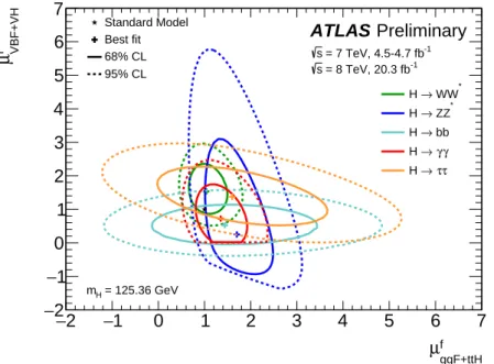
The measurement of the total cross section, extrapolated to the full phase space, based on the fiducial cross section measurements in H → γγ and H → ZZ ∗ → 4` follows a di ff

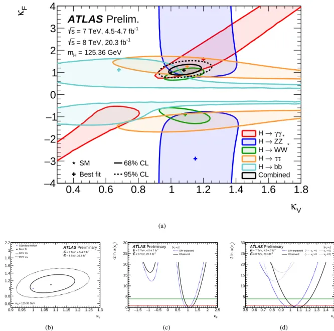
Here the ratio λ lq between leptons and quarks is probed, while vector boson couplings are taken unified as κ V. The indices l, q stand for all leptons and quarks, respectively.

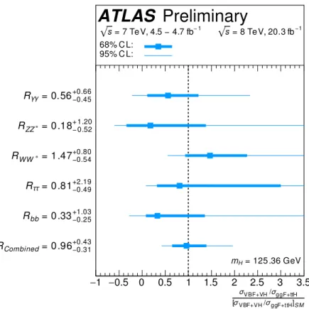
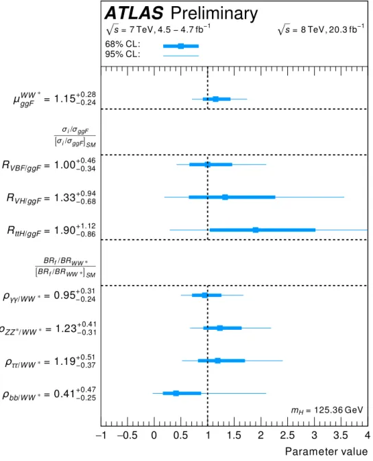
Measurements of relative branching fraction ratios between the H → γγ , H → ZZ (∗) → 4 ` and H → WW (∗) → `ν`ν channels, as well as combined fits testing the fermion

● Incorporation of spontaneous symmetry breaking in gauge field theory = Higgs mechanism:.. ● Leads to prediction of new particle: →

The results of the four problem subscales of the SDQ (emotional symptoms, conduct problems, hyperactivity-inattention, and peer problems), the combined total difficulties score,

The main reason we state this and the next example is to show that Proposition 5 can be used both in a positive sense (if some CSC-compliant normalizer exists, then the

Regional climate model (HIRHAM) | Land surface model (SWET) | Hydrology model (MIKE

Fourier  Transform  Ion  Cyclotron Resonance  Mass