Lattice artefacts and the running of the coupling constant.

arXiv:hep-lat/0009005v2 3 Nov 2000

Lattice artefacts and the running of the coupling constant.

Adrian Patrascioiu

Physics Department, University of Arizona, Tucson, AZ 85721, U.S.A.

Erhard Seiler

Max-Planck-Institut f¨ ur Physik (Werner-Heisenberg-Institut) F¨ ohringer Ring 6, 80805 Munich, Germany (Dated: November 6, 2018)

We study the running of the L¨ uscher-Weisz-Wolff (LWW) coupling constant in the two dimensional O(3) nonlinear σ model. To investigate the continuum limit we refine the lattice spacing from the

1

16

value used by LWW up to

. We find much larger lattice artefacts than those estimated by LWW and that most likely the coupling constant runs slower than predicted by perturbation theory.

A precise determination of the running in the continuum limit would require a controlled ansatz of extrapolation, which, we argue, is not presently available.

PACS numbers: 64.60.Cn, 05.50.+q, 75.10.Hk

The hallmark of QCD is its alleged asymptotic free- dom (AF), that property which expresses the fact that at shorter distances the interactions between quarks and gluons are becoming weaker. This fact however has been established only in perturbation theory (PT), an approx- imation scheme without a mathematical basis and which, moreover, has been shown to be plagued by ambiguities (expectation values of variables of compact support de- pend upon the boundary conditions (b.c.) used to reach the thermodynamic limit) [1].

It is therefore most important to establish whether AF is really a property of QCD in a nonperturbative frame- work. The first step in this direction was taken in 1991 by L¨ uscher, Weisz and Wolff (LWW) [2], who proposed a method to investigate the presnce of AF in the two dimensional (2D) O(N ) nonlinear σ models, which, per- turbatively, are also AF for N ≥ 3. As a coupling con- stant they proposed the following renormalization group invariant:

˜

g ² (β, L) = 2L

(N − 1)ξ(L) (1)

Here ξ(L) is the correlation length of the O(N ) model in an infinite strip of width L with periodic b.c.. It is defined by the following double limit: consider a finite strip of size L × T with periodic b.c. in the direction of size L and arbitrary b.c. in the direction of size T . Then

ξ(L) = −lim x →∞ lim T →∞

x

ln(< s(0) · s(x) >) . (2) For the standard O(N ) action

H i,j = −s(i) · s(j) (3) at inverse coupling constant β, if in eqn.(1) one ex- pressed L in units of the thermodynamic correlation length ξ ∞ (β), then in the limit L → ∞ and β → β crt , holding z = L/ξ ∞ fixed, one would obtain a unique func- tion ¯ g ² (z) describing the running of ¯ g ² with the physical distance z.

As we pointed out in 1992 [3], the interpretation of ¯ g ² as a coupling constant is somewhat misleading since it does not measure the strength of the interaction. Indeed in the the massive continuum limit of a free field theory

¯

g ² (z) is a nontrivial function, running linearly with z.

LWW argued in favour of their choice by pointing out that in PT, to lowest order in the bare (lattice) coupling constant ¯ g ² (L) ∼ _β ¹ . This argument is also problematic since even if β crt = ∞, to construct the continuum limit one would have to let L → ∞ and thus reach a regime where PT in the bare coupling would clearly not be ap- plicable.

Nevertheless ¯ g ² (L, β) is a renormalization group invari- ant and if one would discover that for some β < ∞, ¯ g ² (L) became independent of L for large L, that would mean that at that β the model is critical, which, as we will explain below, would rule out the existence of AF in the massive continuum limit.

In 1991, for the O(3) model, LWW claimed to be able to establish the continuum running of ¯ g ² (L/ξ ∞ (β)) up to physical distances as small as 0.03304(4) and to verify that it approached the perturbative (AF) predic- tion. To achieve this they employed a finite size scal- ing (FSS) technique: one measures ξ(L) at some β and L, then leaving β unchanged, one doubles L and mea- sures ξ(2L). One thus obtains a scaling curve giving

¯

g ² (2L)/¯ g ² (L) versus ¯ g ² (L). This step scaling curve, as LWW called it, allows one to connect small physical dis- tances to large ones (L/ξ ∞ (β) > 7), where the continuum limit of ¯ g ² (L/ξ ∞ (β)) could be reached.

Similar FSS approaches were used in 1993 by Kim [4]

and in 1994 by Caracciolo et al [5] to predict the value

of ξ(β) up to ξ ∼ 10 ⁵ , even though the largest lattices

involved did not exceed L = 512. However whereas these

authors produced their scaling curves simply by observ-

ing that the Monte Carlo (MC) data coming from differ-

ent values of β seemed to fall on the same curve, which

they took as their step scaling curve, the LWW paper

claimed to have really controlled lattice artefacts (the

aproach to the continuum). More precisely the problem

is this: of course if one knew the continuum value of the

2 step scaling curve one could connect small physical dis-

tances to large ones. But in an MC investigation, by ne- cessity, one can only gather data at finite cutoff (1/ξ ∞ (β ) or alternatively 1/L). However the continuum limit re- quires letting ξ ∞ (β) → ∞ and L → ∞. Therefore one must in principle worry about extrapolating the results obtained for the step scaling function at finite cutoff to the continuum limit.

This feat, which the other above quoted authors did not even attempt, was achieved by LWW by assuming a Symanzik type of approach to the continuum limit.

Namely at fixed ¯ g ² they assumed that the step scaling function approaches its continuum limit value as 1/L ² (strictly speaking, inspired by PT, the Symanzik fit in- volves log(L)/L ² , however for 6 ≤ L ≤ 16 the log can be approximated by a constant). They backed this assump- tion with their MC data. However the values of L they used ranged only from 6 ≤ L ≤ 16. The main point of our paper is to show numerical evidence that if one goes to much larger L values, the Symanzik fit does not work and an entirely new picture for the running of ¯ g ² with the physical distance emerges.

Before showing our data, we would like to elaborate on a subtlety having to do with the numerical determi- nation of the correlation length ξ(L). Namely while the definition in eq.(1) is mathematically well defined, one must adopt a computational procedure for implement- ing it. LWW used an L × T lattice with free b.c. in the T -direction, took T = 5L and assumed a pure ex- ponential decay for L < x < T − L (see Appendix B of ref.[2]). We used instead the following numerical esti- mate of the correlation length ξ: let P = (p, 0), p = ^2nπ _T , n = 0, 1, 2, ..., T − 1, T = 10L. Then

ξ = 1

2 sin(π/T )

p G(0)/G(1) − 1 (4) where

G(p) = 1

LT h|ˆ s(P)| ² i; ˆ s(P ) = X

x

e ^{iP x} s(x) (5) It is not clear whether the LWW prescription or the one adopted by us provides an estimate closer to the true ex- ponential correlation length. For finite T the LWW pro- cedure, employing free b.c., is likely to produce a value smaller than the true ξ(L). In the procedure adopted by us, there are two effects of opposite sign, which could bring the result closer to the true exponential correlation length:

1. The periodic b.c. in the T -direction increases the or- der in the system compared to an infinite strip.

2. Since our definition is sensitive to the multiparticle states, for T → ∞ it would produce a value smaller than the true ξ(L). This effect was studied by Campostrini et al [6] using the high temperature expansion and found to be less than 0.2%.

Since we want to compare our data with those of LWW, we show in Fig.1 the resulting step scaling functions com- puted with the two procedures at the same β and L. As

can be seen, within numerical accuracy, at these values of ¯ g ² the two procedures produce similar results.

FIG. 1: Step scaling function ¯ g

(2L)/¯ g

(L) versus g ¯

(L) for L = 20, 40, 80 computed with our method of estimating ξ(L) (solid lines) and with the LWW method (dotted line).

FIG. 2: Step scaling function ¯ g

(2L)/¯ g

(L) versus g ¯

(L) for L = 20. Our MC data are connected by a spline.

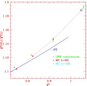
Our results for the step scaling function are shown in Fig.2, Fig.3 and Fig.4 for L = 20, 40 and 80 respectively.

The values were obtained by measuring the correlation

length at given β first on a lattice of size L×10L, then on

2L × 20L. The values of β used (1.815, 1.94, 2.05, 2.16,

3

FIG. 3: Step scaling function ¯ g

(2L)/¯ g

(L) versus ¯ g

(L) for L = 40. Our MC data arew connected by a spline.

FIG. 4: Step scaling function ¯ g

(2L)/¯ g

(L) versus ¯ g

(L) for L = 80 and 160. Our MC data for L = 80 are connected by a spline.

2.27, 2.38 and 2.49) were chosen so that ¯ g ² took values in the range covered by LWW. The figures contain also two benchmarks taken from LWW [2]:

- The 3-loop PT curve.

- The LWW estimated continuum values.

Fig.4 contains also our value for the step scaling func- tion obtained by doubling L from 160 to 320 at ¯ g ² = 1.05397(81). The error bars were estimated as follows:

for each value of β and L we started from a randomly

chosen configuration and ran the improved cluster algo- rithm [7] using 100,000 clusters for thermalization and 1,000,000 clusters for measurements. We then repeated this procedure a minimum of 157 times, except for the value at L = 320 which contains only 74 runs. We com- puted the average value over these samples of G(0) and G(1) and from them ξ(L). Since ξ(L) is a nonlinear func- tion of G(0) and G(1), we estimated the error for ξ(L) and ¯ g ² (L) from our sample of independent values by the jack-knife method. The data for ˜ g ² (L) that were used in the figures are given in Tab.1.

Our data do not agree with the LWW prediction [2]

for the step scaling function. The latter were obtained by extrapolating the MC values obtained by taking L between L = 6 and L = 16 via a second order polynomial in _L ¹

. We did not display the LWW values for 6 ≤ L ≤ 16 because of lack of space. However when combined with our values, they reveal a rather complicated approach to the continuum. This is not an unexpected fact. Indeed if L is sufficiently small at given β, the (asymmetric) lattice is strongly ordered in the transverse (shorter) direction.

On the other hand, as we emphasized several years ago [8], since in the continuum limit one must let L → ∞ and the Mermin-Wagner theorem guarantees the restoration of the O(N) symmetry in that limit for any finite β, clearly for L sufficiently large this ‘perturbative’ regime, of spins highly ordered in the transverse direction, cannot persist.

In fact we showed in [8] that even if β crt = ∞, as predicted by PT, the spins would cease to be highly or- dered in the transverse direction for L sufficiently large.

Indeed bare PT itself provides a clue as to the distance over which the spins remain well ordered since to lowest order one has

hs(0) · s(x)i = 1 − N − 1

β D(x) (6)

and to a good approximation D(x) = ¹ ₄ + _2π ¹ ln(x). Thus bare PT suggests that spins are well ordered over dis- tances O(exp([2πβ/(N − 1)]). On the other hand the AF formula predicts ξ = O(exp[2πβ/(N − 2)]). Thus at fixed physical distance ( _ξ(L) ^L ), in taking the continuum limit one would surely leave the regime in which PT in the bare coupling is applicable.

Returning now to the pattern of lattice artefacts, ini-

tially, if β is large enough, at small enough L, they should

follow the Symanzik pattern used by LWW because the

system is essentially in a PT regime. This regime has

nothing to do with the true approach to the continuum,

which occurs only when L is sufficiently large (for given

β) so that the O(N ) symmetry becomes approximately

true. How the true continuum limit is approached can

be model dependent. For instance in the Ising model

there are good reasons to expect a 1/L ² leading behavior

[9]. On the other hand in the O(2) model there are both

theoretical [10] and numerical reasons [11] to expect a

1/ ln(L) approach.

4 It is reasonable to expect that the O(3) model, enjoy-

ing a continuous symmetry, behaves as the O(2), not as the Ising model. We have attempted a _ln(L) ¹ fit to our data but could not obtain a reliable continuum value.

(We encountered a similar situation in investigating the renormalized coupling g R in the O(3) model [12]. The case of the O(2) model is simpler to handle because the theory predicts both the continuum value and the leading correction [11].) Even though we do not have a predic- tion for the continuum step scaling function, our results do not corroborate the original prediction of LWW and suggest that most likely the nonperturbative running of

¯

g ² is slower than predicted by PT. This situation is con- sistent with, though in no way proving, the existence of a transition to a massless phase at finite β crt , as argued by us recently [13]. In that paper we also proved rigor- ously that for the standard action, the massive contin- uum limit cannot be AF if β crt < ∞. The result follows from a Ward identity and the reflection positivity of the standard action.

Finally, regarding the running of α s (Q) in QCD 4 , all we can say is that the Symanzik type of fit for the ap-

proach to the continuum has no justification there ei- ther. Indeed, that fit is inspired by PT. If in fact lat- tice QCD 4 does undergo a deconfining zero temperature transition at nonzero (bare) coupling, so that the run- ning of α s (Q) does not follow PT, there is no reason to expect the lattice artefacts to follow the Symanzik ansatz.

Therefore it would be very useful if the lattice community employed its resources to establish first the true cutoff ef- fects and the true running of α s in the pure Yang-Mills theory by going to larger L, before attempting to handle dynamical fermions; the latter unavoidably can only be done on minuscule lattices, and using the Symanzik fit to extrapolate to the continuum can be misleading, as we have found. As we said many years ago [14], we expect that in the four dimensional Yang-Mills theory as well as in QCD 4 there exists a nontrivial fixed point and that α s (Q) runs slower than predicted by PT, with the effect becoming pronounced by 1 TeV or less.

Acknowledgement: We benefitted from numerous dis- cussions with Peter Weisz regarding the LWW paper.

AP is grateful to the Werner-Heisenberg-Institut for its hospitality.

Tab.1: Monte Carlo data for g ˜ ² (β, L)

β 1.815 1.94 2.05 2.16 2.27 2.38

L = 20 1.06185(78) .91115(67) .81616(70) .74170(56)

L = 40 1.27230(85) 1.04334(76) .91530(68) .81901(63) .74419(57)

L = 80 1.24174(85) 1.04778(72) .91907(70) .82404(60) .74811(53) L = 160 1.24497(100) 1.05398(81) .92457(69) .82564(58)

L = 320 1.2530(15)

[1] A. Patrascioiu and E. Seiler, Phys.Rev.Lett. 74 (1995) 1924.

[2] M. L¨ uscher, P. Weisz and U. Wolff, Nucl.Phys. B359 (1991) 221.

[3] A. Patrascioiu and E. Seiler, Nuovo Cim. 107A (1994) 765.

[4] J.-K. Kim, Phys.Rev.Lett. 70 (1993) 1735.

[5] S. Caracciolo, R. G. Edwards, A. Pelissetto and A. Sokal, Phys.Rev.Lett. 75 (1995) 1891.

[6] M. Campostrini, A. Pelissetto, P. Rossi and E. Vicari,, Phys.Lett. B402 (1997) 141.

[7] U. Wolff, Nucl.Phys. B334 (1990) 581.

[8] A. Patrascioiu and E. Seiler , J. Stat. Phys. 89 (1997) 947.

[9] M. N. Barber, in Phase Transitions and Critical Phenom-

ena vol.8 ed. C. Domb and J. L. Lebowitz (1983).

[10] J. M. Kosterlitz, J.Phys. C7 (1974) 1046.

[11] M. Hasenbusch, An Improved Estimator for the Cor- relation Function of 2D Nonlinear Sigma Models hep- lat/9408019 (1994).

[12] J. Balog, M. Niedermaier, F. Niedermayer, A. Pa- trascioiu, E. Seiler and P. Weisz, Nucl. Phys. B576 (2000) 517.

[13] A. Patrascioiu and E. Seiler, Absence of asymptotic free- dom in nonabelian models hep-th/0002153 (2000).

[14] A. Patrascioiu and E. Seiler, in Rencontres de Physique

de la Vall´ ee d’Aoste ed. M.Greco, Editions Fronti`eres

(1992) p.125.