Updated coupling measurements of the Higgs boson with the ATLAS detector using up to 25 fb − 1 of proton-proton collision data

A TLAS-CONF-2014-009 17/05/2014

ATLAS NOTE

ATLAS-CONF-2014-009

March 20, 2014 Revision: May 5, 2014

Updated coupling measurements of the Higgs boson with the ATLAS detector using up to 25 fb ^{− 1} of proton-proton collision data

The ATLAS Collaboration

Abstract

This note is a presentation of an update of the measurements of the signal strengths and couplings of the Higgs boson using the full 2011 and 2012 pp collision data sample recorded by the ATLAS experiment at the LHC at √

s = 7 TeV, respectively √

s = 8 TeV, for the channels H→ γγ, H→ ZZ

→ 4`, H→ WW

→ `ν`ν and H → b b, and the full 2012 ¯ pp collision data sample at √

s = 8 TeV for the H → ττ channel. The combined signal strength is determined to be µ = 1.30 ± 0.12 (stat)

(sys) at a Higgs boson mass of 125.5 GeV. Ev- idence for direct decay into fermions is found at the 3.7σ level from the combination of the H → b b ¯ and H → ττ channels with a signal strength of µ

= 1.09 ± 0.24 (stat)

(sys).

Measurements of production and decay mode specific signal strengths and Higgs boson cou- pling determinations in various benchmark models show good agreement with the Standard Model Higgs boson hypothesis.

The coloring scheme of the likelihood contour plot of Figure 5(b) for the VH(bb) channel has been corrected.

c

Copyright 2014 CERN for the benefit of the ATLAS Collaboration.

Reproduction of this article or parts of it is allowed as specified in the CC-BY-3.0 license.

1 Introduction

The observation of a new particle in the search for the Standard Model (SM) Higgs boson at the LHC, reported by the ATLAS [1] and CMS [2] Collaborations, is a milestone in the quest to understand elec- troweak symmetry breaking. Precision measurements of the properties of the new boson are of critical importance. Among its key properties are the couplings to each of the SM fermions and bosons. In Ref. [3] the ATLAS Collaboration reported first measurements of the mass of the particle and its cou- pling properties using the diboson decay modes to γγ, ZZ

and WW

. In Ref. [4] the CMS Collaboration reported on the first evidence for the direct decay of the Higgs boson to fermions. Since the publication on the diboson channels, the ATLAS Collaboration has made available important results on fermionic channels, namely H → b b ¯ [5] and H → ττ [6]. An update of the measurements of the coupling properties of the Higgs boson including the new fermionic modes is presented in this document. The analysis uses the full 2011 and 2012 pp collision data sample recorded by the ATLAS experiment at

√ s = 7 TeV and √

s = 8 TeV, respectively, for the channels H→ γγ, H→ ZZ

→ 4`, H→ WW

→ `ν`ν [3] and H → b b ¯ [5], and the full 2012 pp collision data sample at √

s = 8 TeV for the H → ττ chan- nel [6].

The results are based on the same statistical model as defined in Refs. [1, 3]. The aspects of the individual channels relevant for these measurements are briefly summarised in Section 2. The statisti- cal procedure and the treatment of systematic uncertainties are outlined in Section 3. In Section 4 the measured yields are analysed in terms of the signal strengths, for different production and decay modes and their combinations. Finally, in Section 5 the couplings of the newly discovered boson are tested through fits to the observed data. These studies aim to probe, under the assumptions described in the text, the Lagrangian structure in the vector boson and fermion sectors, specifically couplings to fermions and bosons, the ratio of couplings to the W and Z bosons, to up- and down-type fermions, to leptons and quarks, and the e ff ective couplings to photons and gluons. A limit is set on the branching ratio to invisible or undetected decay modes. In addition, generic coupling models are explored.

2 Input Channels

The determination of the integrated luminosity for the 2012 dataset has been improved with respect to that of Ref. [3], with a new value of 20.3 fb

with an uncertainty of 2.8%. This uncertainty is derived, following the same methodology as that detailed in Ref. [7], from a preliminary calibration of the luminosity scale derived from beam-separation scans performed in November 2012. The H→ ZZ

→ 4`, H→ γγ and H→ WW

→ `ν`ν results are taken from the analysis in Ref. [3], using the full 2011 and 2012 datasets, and taking into account the new luminosity measurement for 2012. The H → b b ¯ and H → ττ results, documented in Ref. [5] and Ref. [6], respectively, have been evaluated at the measured mass of 125.5 GeV as obtained from the H→ ZZ

→ 4` and H→ γγ [3] channels, resulting in a change of the extracted signal strengths of 2 − 3% caused by the change in the cross sections and branching ratios with respect to the reference mass of 125 GeV used in Refs. [5, 6].

The event selections of the vector boson fusion (VBF) category of the H→ WW

→ `ν`ν analysis in

Ref. [3] and the dilepton final state of the H → ττ analysis in Ref. [6] have a small overlap. In order

to render the two signal selections mutually exclusive for this combination, a cut on the reconstructed

ditau invariant mass m

< m

− 25 GeV is added to the H→ WW

→ `ν`ν VBF selection and a cut on

m

> m

− 25 GeV is added to the dilepton H → ττ selection. For this purpose, m

is calculated

from the lepton momenta and E

in the collinear approximation [6]. Application of this cut has no

impact on the events in the bins with the best signal-to-background ratio (highest score of the multivariate

discriminant) in the H → ττ analysis. In the VBF H→ WW

→ `ν`ν analysis the cut removes most of

the H → ττ signal contamination, but also removes ∼10% of the expected VBF H→ WW

→ `ν`ν signal

events. However, these removed H→ WW

→ `ν`ν signal events are mostly retained within the H → ττ analysis selection.

The H→ WW

→ `ν`ν channel also contaminates the H → ττ selection. In Ref. [6] this was treated as a background, with SM signal strength. In the present study, this contamination is rescaled by the measured H→ WW

→ `ν`ν signal strength.

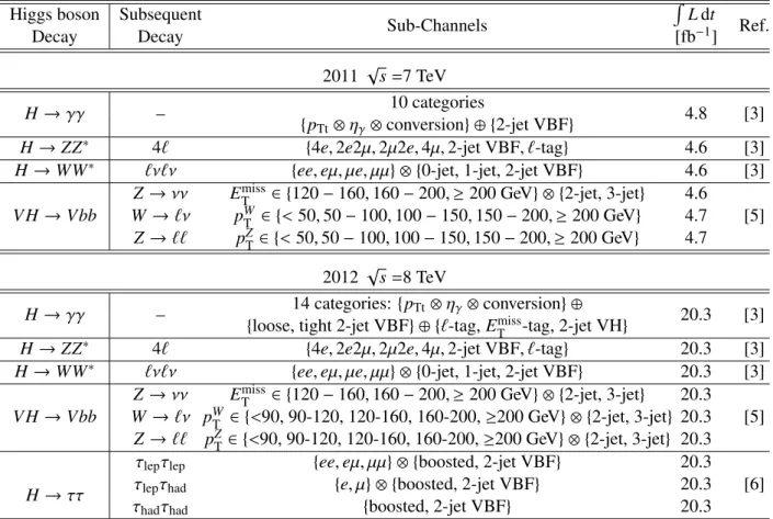
The final states and channel categories considered in this analysis are summarised in Table 1.

3 Statistical Procedure

The statistical treatment of the data is described in Refs. [8–12]. Hypothesis testing and confidence in- tervals are based on the Λ(α) profile likelihood ratio [13] test statistic. The latter depends on one or more parameters of interest α, such as the Higgs boson signal strength µ normalised to the SM expectation (so that µ = 1 corresponds to the SM Higgs boson hypothesis and µ = 0 to the background-only hypothe- sis), Higgs boson mass m

, coupling strength scale factors κ and their ratios λ , as well as on nuisance

Table 1: Summary of the individual channels entering the combined results presented here. In channels sensitive to associated production of the Higgs boson, V indicates a W or Z boson. The symbols ⊗ and ⊕ represent direct products and sums over sets of selection requirements, respectively. The abbreviations listed here are described in the corresponding references indicated in the last column. For the H→ γγ channel the variables p

and η

are defined in Ref. [3].

Higgs boson Subsequent

Sub-Channels

R L dt

Decay Decay [fb

] Ref.

2011 √

s =7 TeV

H → γγ – 10 categories

4.8 [3]

{ p

⊗ η

⊗ conversion} ⊕ {2-jet VBF}

H → ZZ

4` {4e, 2e2µ, 2µ2e, 4µ, 2-jet VBF, `-tag} 4.6 [3]

H → WW

`ν`ν {ee, eµ, µe, µµ} ⊗ {0-jet, 1-jet, 2-jet VBF} 4.6 [3]

V H → Vbb

Z → νν E

∈ {120 − 160, 160 − 200, ≥ 200 GeV} ⊗ {2-jet, 3-jet} 4.6

W → `ν p

∈ {< 50, 50 − 100, 100 − 150, 150 − 200, ≥ 200 GeV} 4.7 [5]

Z → `` p

∈ {< 50, 50 − 100, 100 − 150, 150 − 200, ≥ 200 GeV } 4.7 2012 √

s =8 TeV

H → γγ – 14 categories: {p

⊗ η

⊗ conversion } ⊕

20.3 [3]

{loose, tight 2-jet VBF} ⊕ {`-tag, E

-tag, 2-jet VH}

H → ZZ

4` {4e, 2e2µ, 2µ2e, 4µ, 2-jet VBF, `-tag} 20.3 [3]

H → WW

`ν`ν {ee, eµ, µe, µµ} ⊗ {0-jet, 1-jet, 2-jet VBF} 20.3 [3]

V H → Vbb

Z → νν E

∈ { 120 − 160, 160 − 200, ≥ 200 GeV } ⊗ { 2-jet, 3-jet } 20.3 W → `ν p

∈ {<90, 90-120, 120-160, 160-200, ≥200 GeV} ⊗ {2-jet, 3-jet} 20.3 [5]

Z → `` p

∈ {<90, 90-120, 120-160, 160-200, ≥200 GeV} ⊗ {2-jet, 3-jet} 20.3 H → ττ

τ

τ

{ee, eµ, µµ} ⊗ {boosted, 2-jet VBF} 20.3 τ

τ

{e, µ} ⊗ { boosted, 2-jet VBF } 20.3 [6]

τ

τ

{boosted, 2-jet VBF} 20.3

parameters θ,

Λ(α) = L α , θ(α) ˆˆ

L( ˆ α, θ) ˆ . (1)

The likelihood functions in the numerator and denominator of the above equation are built using sums of signal and background probability density functions (pdfs) in the discriminating variables. These variables are the γγ, 4` and 2b-jet masses for H→ γγ, H→ ZZ

→ 4` and H → b b, respectively, the ¯ transverse mass m

(defined in Ref. [3]) for the H→ WW

→ `ν`ν channel and a multivariate discriminant output distribution for H → ττ. The pdfs are derived from MC simulation for the signal and from both data and simulation for the background. Likelihood fits to the observed data are done for the parameters of interest. The single circumflex in Eq. 1 denotes the unconditional maximum likelihood estimate of a parameter and the double circumflex denotes the conditional maximum likelihood estimate for given fixed values of the parameters of interest α.

Systematic uncertainties and their correlations [8] are modelled by introducing nuisance parameters θ described by likelihood functions associated with the estimate of the corresponding effect. The choice of the parameters of interest depends on the test under consideration, with the remaining parameters being

“profiled”, i.e., similarly to nuisance parameters they are set to the values that maximise the likelihood function for the given fixed values of the parameters of interest.

Asymptotically, a test statistic −2 ln Λ (α) of several parameters of interest α is distributed as a χ

distribution with n degrees of freedom, where n is the dimensionality of the vector α. In particular, the 100(1 − β)% confidence level (CL) contours are defined by − 2 ln Λ(α) < k

, where k

satisfies P(χ

> k

) = β. For two degrees of freedom the 68% and 95% CL contours are given by −2 ln Λ(α) = 2.3 and 6.0, respectively. All results presented in the following sections are based on likelihood evaluations and therefore give only approximate CL intervals.

For the measurements in the following sections the compatibility with the Standard Model, p

, is quantified using the p-value obtained from the profile likelihood ratio Λ (α = α

), where α is the set of parameters of interest and α

are their Standard Model values. For a given coupling benchmark model, α is the set of κ

and λ

parameters of that model, where the indices i, j refer to the parameters of interest of the model. All other parameters are treated as independent nuisance parameters.

4 Signal Strength in Production and Decay Modes

This section focuses on the measurement of the global signal strength parameter µ and the individual signal strength parameters µ

which depend upon the Higgs boson production mode i and the decay channel f , for a fixed mass hypothesis corresponding to the measured value m

= 125.5 GeV [3]. The parameters µ and µ

are determined from a fit to the data using the profile likelihood ratio Λ (µ) (see Eq. 1).

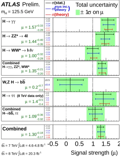
The results are shown in Fig. 1, where the signal strengths measured in the five individual channels are presented

. The signal strength normalised to the SM expectation, obtained by combining the three diboson channels, was published in Ref. [3] as µ

= 1.33 ± 0.14 (stat) ± 0.15 (sys). With the changes described in Section 2, this value is updated to µ

= 1.35 ± 0.14 (stat)

(sys). The combination of the two fermion channels H → b b ¯ and H → ττ yields a signal strength

µ

= 1.09 ± 0.24 (stat)

(sys),

1

Whenever probabilities are translated into the number of Gaussian standard deviations the two-sided convention is chosen.

2

The results for H→ γγ, H→ ZZ

→ 4` and H → b b ¯ are taken from the individual analyses, while the results for

H → WW

→ `ν`ν and H → ττ are taken from the combination of these two channels with independent signal strengths for

the two final states in order to take the signal cross contamination into account (see Section 2).

corresponding to 3.7σ evidence for the direct decay of the Higgs boson into fermions.

Finally, the signal strength, obtained by combining all five channels, is:

µ = 1.30 ± 0.12 (stat)

(sys).

A significant component of the systematic uncertainty is associated to the theoretical values of the cross sections and branching ratios. The uncertainty on the cross section amounts to ± 7%, dominated by uncertainties on the QCD renormalisation and factorisation scales and the parton distribution function (PDF) for the gluon-gluon fusion process (ggF). The uncertainty on the mass measurement of ±0.6 GeV reported in Ref. [3] leads to a ± 3% uncertainty on µ.

The compatibility between this measurement and the SM Higgs boson expectation (µ = 1) is about 7%; the use of a flat likelihood for the ggF QCD scale systematic uncertainty in the quoted ±1σ interval yields a similar level of compatibility (8%) with the µ = 1 hypothesis. The overall compatibility between the signal strengths measured in the five final states and the SM predictions is about 11%. Both the central value of µ and the SM compatibility have changed little with respect to the diboson measurements of Ref. [3]. The contribution of the diboson channels still dominates the measurement, and the combination of the H → b b ¯ and H → ττ modes has a compatible measured value of µ .

The measurements of the signal strengths described above do not give direct information on the rel- ative contributions of the different production mechanisms. Furthermore, fixing the ratios of the produc- tion cross sections for the various processes to the values predicted by the Standard Model may conceal di ff erences between data and theoretical predictions. Therefore, in addition to the signal strengths of di ff erent decay channels, the signal strengths of di ff erent production processes contributing to the same decay channel

are determined, exploiting the sensitivity offered by the use of event categories in the analyses of all the channels.

The data are fitted separating the VBF and VH processes, which involve the Higgs boson coupling to vector bosons, from the ggF and ttH processes, which involve the Higgs boson coupling to fermions (mainly the top-quark).

Two signal strength parameters, µ

= µ

= µ

and µ

= µ

= µ

, which scale the SM-predicted rates to those observed, are introduced for the channels H→ γγ, H→ ZZ

→ 4`, H→ WW

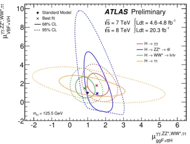
→ `ν`ν and H → ττ indexed by the parameter f . The H → b b ¯ final state is not included, as the current analysis is only sensitive to the V H production mode, and not to the VBF or ggF production modes. The results are shown in Fig. 2. The 95% CL contours of the measurements are consistent with the SM expectation.

A combination of all four channels provides a higher-sensitivity test of the theory. This can be done in a model-independent way (i.e. without assumptions on the Higgs boson branching ratios) by measuring the ratios µ

/µ

for the individual final states and their combination. The result of the fit to the data with the likelihood Λ(µ

/µ

) is

µ

/µ

= 1.4

(stat)

(sys).

The results for individual channels and their combination are shown in Fig. 3. Good agreement with the SM expectation is observed. The main components of the systematic uncertainty

come from the theoretical predictions for the ggF contributions to the various categories and jet multiplicities.

The changes in the results of the H→ WW

→ `ν`ν and H → ττ channels, respectively from Ref. [3]

and Ref. [6], are mainly due to the separation of their VBF signal regions by the cut on m

described in

3

Such an approach avoids model assumptions needed for a consistent parameterisation of production and decay channels in terms of Higgs boson couplings.

4

Such a separation is possible under the assumption that the kinematic properties of these production modes agree with the SM predictions within uncertainties.

5

A component of the statistical uncertainty in the results for µ

/µ

in Ref. [3] was incorrectly counted as sys-

tematic error there. It is corrected here.

µ ) Signal strength ( -0.5 0 0.5 1 1.5 2 ATLAS Prelim.

Ldt = 4.6-4.8 fb-1

∫

= 7 TeV s

Ldt = 20.3 fb-1

∫

= 8 TeV s

= 125.5 GeV m

0.28 -

0.33

= 1.57

µ γ γ

→ H

0.12 -

0.17 +

0.18 -

0.24 +

0.22 -

0.23 +

0.35 -

0.40

= 1.44

µ

→ 4l ZZ*

→ H

0.10 -

0.17 +

0.13 -

0.20 +

0.32 -

0.35 +

0.29 -

0.32

= 1.00

µ ν ν l

→ l WW*

→ H

0.08 -

0.16 +

0.19 -

0.24 +

0.21 -

0.21 +

0.20 -

0.21

= 1.35

, ZZ*, WW*

µ

γ

→ H Combined

0.11 -

0.13 +

0.14 -

0.16 +

0.14 -

0.14 +

0.6 -

0.7

= 0.2

µ b

→ b W,Z H

<0.1

±0.4

±0.5

0.4 -

0.5

= 1.4

µ

(8 TeV data only)

τ τ

→ H

0.1 -

0.2 +

0.3 -

0.4 +

0.3 -

0.3 +

0.32 -

0.36

= 1.09

τ

µ

→b H

Combined

0.04 -

0.08 +

0.21 -

0.27 +

0.24 -

0.24 +

0.17 -

0.18

= 1.30

µ

Combined

0.08 -

0.10 +

0.11 -

0.14 +

0.12 -

0.12 +

Total uncertainty µ σ on

± 1

(stat.) σ

theory

)

sys inc.

σ (

(theory) σ

Figure 1: The measured signal strengths for a Higgs boson of mass m

= 125.5 GeV, normalised to the SM expectations, for the individual final states and various combinations. The best-fit values are shown by the solid vertical lines. The total ±1σ uncertainties are indicated by green shaded bands, with the individual contributions from the statistical uncertainty (top), the total (experimental and theoretical) systematic uncertainty (middle), and the theory uncertainty (bottom) on the signal strength (from QCD scale, PDF, and branching ratios) shown as superimposed error bars. The measurements are based on Refs. [3, 5, 6], with the changes mentioned in the text.

Section 2. In the H → ττ channel, the ratio µ

/µ

has an infinite 1σ upper bound, because the signal is almost only observed in the VBF mode, hence the ggF denominator can be arbitrarily small.

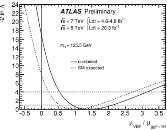
To test the sensitivity to VBF production alone, the data are also fitted with the ratio µ

/µ

. In order not to influence the VBF measurement through the VH categories, the parameter µ

/µ

is treated independently and profiled. A value of

µ

/µ

= 1.4

(stat)

(sys)

is obtained from the combination of the four channels (Fig. 4). This result provides evidence at the 4.1σ

level that a fraction of Higgs boson production occurs through VBF.

τ τ ,ZZ*,WW*, γ γ ggF+ttH

µ

-2 -1 0 1 2 3 4 5 6

ττ,ZZ*,WW*,γγ VBF+VH

µ

-2 0 2 4 6 8

10

Best fit 68% CL 95% CL

γ γ

→ H

→ 4l ZZ*

H →

ν νl

→ l WW*

→ H

τ τ

→ H

Preliminary ATLAS

Ldt = 4.6-4.8 fb-1

∫

= 7 TeV s

Ldt = 20.3 fb-1

∫

= 8 TeV s

= 125.5 GeV mH

Figure 2: Likelihood contours in the (µ

, µ

) plane for the channels f = H→ γγ, H→ ZZ

→ 4`, H→ WW

→ `ν`ν, H → ττ and a Higgs boson mass m

= 125.5 GeV. The sharp lower edge of the H→ ZZ

→ 4` contours is due to the small number of events in this channel and the require- ment of a positive pdf. The best-fit values to the data (×) and the 68% (full) and 95% (dashed) CL contours are indicated, as well as the SM expectations ( + ).

5 Coupling fits

In the previous section signal strength scale factors µ

for given Higgs boson production or decay modes are discussed. However, for a measurement of Higgs boson couplings, production and decay modes cannot be treated independently. Scenarios with a consistent treatment of Higgs boson couplings in production and decay modes are studied in this section. All uncertainties on the best-fit values shown in this Section take into account both experimental and theoretical systematic values.

5.1 Framework for coupling scale factor measurements

Following the leading order (LO) tree level motivated framework and benchmarks recommended in Ref. [14], measurements of coupling scale factors are implemented for the combination of all analyses and channels summarised in Table 1. This framework is based on the following assumptions:

• The signals observed in the di ff erent search channels originate from a single narrow resonance with a mass near 125.5 GeV. The case of several, possibly overlapping, resonances in this mass region is not considered.

• The width of the assumed Higgs boson near 125.5 GeV is neglected, i.e. the zero-width approxi- mation is used. Hence the product σ × BR(i → H → f ) can be decomposed in the following way for all channels:

σ × BR(i → H → f ) = σ

· Γ

Γ

,

where σ

is the production cross section through the initial state i, Γ

the partial decay width into the final state f and Γ

the total width of the Higgs boson.

• Only modifications of couplings strengths, i.e. of absolute values of couplings, are taken into

account, while the tensor structure of the couplings is assumed to be the same as in the SM. This

ggF+ttH

µ

VBF+VH / µ

0 1 2 3 4 5

ATLAS Prelim.

Ldt = 4.6-4.8 fb-1

∫

= 7 TeV s

Ldt = 20.3 fb-1

∫

= 8 TeV s

= 125.5 GeV m

0.6 -

0.8

= 1.2

ggF+ttH

µ^VBF+VH µ

γ γ

→ H

σ 1

σ 2

0.2 -

0.2 +

0.2 -

0.4 +

0.5 -

0.7 +

0.9 -

2.4

= 0.6

ggF+ttH

µ^VBF+VH µ

→ 4l ZZ*

→ H

σ 0.2 1

- 0.3 +

0.2 -

0.6 +

0.9 -

2.3 +

1.0 -

1.9

= 1.8

ggF+ttH

µ^VBF+VH

µ

WW* → l ν l ν

→ H

σ 0.2 1

- 0.5 +

0.4 -

1.3 +

0.9 -

1.4 +

1.2 -

∞

= 1.7

ggF+ttH

µ^VBF+VH µ

τ τ

→ H

0.3 -

∞ +

0.6 -

∞ +

1.0 -

5.3 +

0.5 -

0.7

= 1.4

ggF+ttH

µ^VBF+VH µ

Combined

σ 1

σ 2

0.1 -

0.2 +

0.2 -

0.4 +

0.4 -

0.5 +

Total uncertainty σ

± 1 ± 2 σ

(stat.) σ

theory

)

sys inc.

σ (

(theory) σ

Figure 3: Measurements of the µ

/µ

ratios for the individual final states and their combi- nation, for a Higgs boson mass m

=125.5 GeV. The best-fit values are represented by the solid vertical lines, with the total ±1σ and ±2σ uncertainties indicated by the green and yellow shaded bands, re- spectively, and the statistical uncertainties by the superimposed horizontal error bars. The numbers in the second column specify the contributions of the statistical uncertainty (top), the total (experimental and theoretical) systematic uncertainty (middle), and the theoretical uncertainty (bottom) on the signal cross section (from QCD scale, PDF, and branching ratios) alone. For a more complete illustration, the likelihood curves from which the total uncertainties are extracted are overlaid. The measurements are based on Refs. [3, 6], with the changes mentioned in the text.

means in particular that the observed state is assumed to be a CP-even scalar as in the SM (this assumption was tested by both the ATLAS [15] and CMS [16] Collaborations).

The LO-motivated coupling scale factors κ

are defined in such a way that the cross section σ

and the partial decay width Γ

associated with the SM particle j scale with the factor κ

when compared to the corresponding SM prediction. Details can be found in Refs. [14, 17].

In some of the fits the effective scale factors ^κ

and κ

for the processes H → γ γ and gg → H, which

are loop-induced in the SM, are treated as a function of the more fundamental coupling scale factors κ

,

κ

, κ

, and similarly for all other particles that contribute to these SM loop processes. In these cases

the scaled fundamental couplings are propagated through the loop calculations, including all interference

e ff ects, using the functional form derived from the SM. Similarly the scaling of the VBF cross section

ggF+ttH

µ

VBF / µ

-0.5 0 0.5 1 1.5 2 2.5 3 3.5

Λ-2 ln

0 2 4 6 8 10 12 14 16 18 20 22 24

combined SM expected

Preliminary ATLAS

Ldt = 4.6-4.8 fb-1

∫ = 7 TeV s

Ldt = 20.3 fb-1

∫ = 8 TeV s

= 125.5 GeV mH

Figure 4: Likelihood curve for the ratio µ

/µ

for the combination of the H → γγ, H→ ZZ

→ 4`, H→ WW

→ `ν`ν and H → ττ channels and a Higgs boson mass m

= 125.5 GeV. The parameter µ

/µ

is profiled in the fit. The dashed curve shows the SM expectation. The horizontal dashed lines indicate the 68% and 95% CL.

and the total width scale factor κ

are expressed as functions of the more fundamental coupling scale factors in some fits. To a very good approximation, the relevant expressions for m

= 125.5 GeV are:

κ

∼ 1.59 · κ

− 0.66 · κ

κ

+ 0.07 · κ

(2) κ

∼ 1.06 · κ

− 0.07 · κ

κ

+ 0.01 · κ

(3)

κ

∼ 0.74 · κ

+ 0.26 · κ

(4)

κ

∼ 0.57 · κ

+ 0.22 · κ

+ 0.09 · κ

+ 0.06 · κ

+ 0.03 · κ

+ 0.03 · κ

. (5) For details and the exact expressions used, see Appendix A and Ref. [14].

The assumptions made for the various measurements are summarised in Table 2 and discussed in the next sections together with the results. The functional dependence of the signal strengths on the effective scale factors κ

is explicated for each benchmark model considered and for the most important Higgs boson production and decay modes in Appendix A.

5.2 Fermion versus vector (gauge) couplings

This benchmark is an extension of the fit to the single parameter µ, where different strengths for the fermion and vector couplings are probed. It assumes that only SM particles contribute to the H→ γγ and gg → H vertex loops, and modifications of the coupling strength factors for fermions and vector bosons are propagated through the loop calculations. The fit is performed in two variants, with and without the assumption that the total width of the Higgs boson is given by the sum of the known SM Higgs boson decay modes (modified in strength by the appropriate fermion and vector coupling scale factors).

5.2.1 Only SM contributions to the total width

The fit parameters are the coupling scale factors κ

for all fermions and κ

for all vector couplings:

κ

= ^κ

= ^κ

κ

= ^κ

= ^κ

= ^κ

= ^κ

.

As only SM particles are assumed to contribute to the gg → H vertex loop in this benchmark, the gluon

fusion process depends directly on the fermion scale factor κ

. The relevant scaling formulae can be

found in Appendix A.1.1.

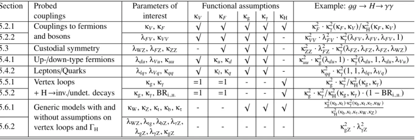
Table 2: Summary of the coupling benchmark models discussed in this note, where λ

= ^κ

/ κ

, κ

= κ

κ

/ κ

, and the functional dependence assumptions are: κ

= κ

= κ

, κ

= κ

= κ

= κ

(and similarly for the other fermions), κ

= ^κ

( κ

, κ

), κ

= ^κ

( κ

, κ

, κ

, κ

), and κ

= ^κ

( κ

). The tick marks indicate which assumptions are made in each case. The last column shows, as an example, the relative couplings involved in the gg → H→ γγ process (see Appendix A for more details).

Section Probed Parameters of Functional assumptions Example: gg → H→ γγ

couplings interest

5.2.1 Couplings to fermions and bosons

κV

,

√ √ √ √ √

κ²_F

·

(

,

)/

(

,

)

5.2.2

,

√ √ √ √

-

·

·

(

,

,

, 1)

5.3 Custodial symmetry

,

,

- √ √ √

-

·

·

(

,

,

,

) 5.4.1 Up-/down-type fermions

,

,

√

κu

,

√ √

-

·

(

, 1) ·

(

, 1,

,

) 5.4.2 Leptons / Quarks

,

,

√

,

√ √

-

·

(1, 1,

,

)

5.5.1 Vertex loops

,

=1 =1 - - √

κ²_g

·

/

(

,

) 5.5.2 + H → inv./undet. decays

,

, BR

=1 =1 - - √

κ²_g

·

γ

/

(

,

) · (1 − BR

) 5.6.1 Generic models with and

without assumptions on vertex loops and Γ

κW

,

,

,

,

- - √ √ √

5.6.2

,

,

,

,

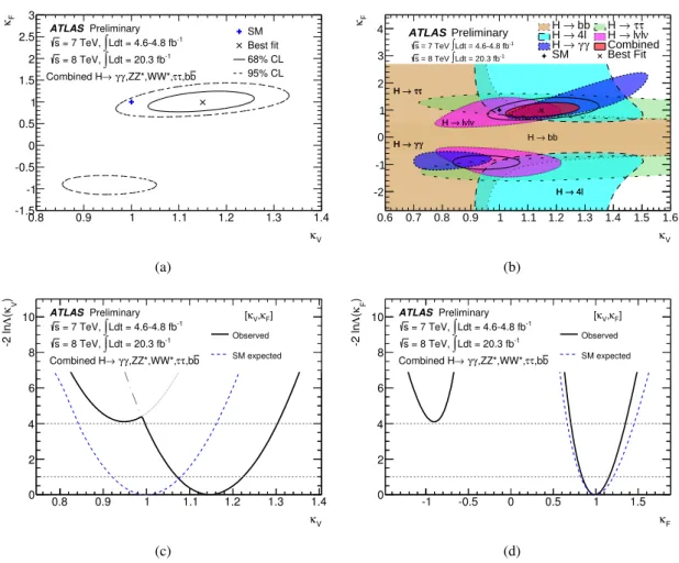
λgZ

,

,

- - - - -

·

Figure 5 shows the results for this benchmark. Only the relative sign between κ

and κ

is physical and hence in the following only κ

> 0 is considered, without loss of generality. Sensitivity to this relative sign is gained from the negative interference between the loop contributions of the W boson and the t quark in the H→ γγ decay (see Eq. 2). As can be seen in Fig. 5(a) the fit prefers the SM-like minimum with a positive relative sign, while the local minimum with negative relative sign is disfavoured at the ∼ 2σ level. Figure 5(b) illustrates how the H→ γγ, H → ZZ

, H → WW

, H → ττ and H → b b ¯ channels contribute to the combined measurement. The likelihoods are given in Figs. 5(c) and 5(d), as a function of κ

when κ

is profiled, and as a function of κ

when κ

is profiled. Figure 5(d) shows in particular to what extent the sign degeneracy is resolved.

The best-fit values and uncertainties, when the other parameter is profiled, are:

κ

= 1.15 ± 0.08 κ

= 0.99

.

The two-dimensional compatibility of the SM hypothesis with the best-fit point is 10%. With respect to the diboson final state combination in Ref. [3], by coincidence the central value is almost unchanged, while the uncertainty on κ

is reduced substantially.

5.2.2 No assumption on the total width

The assumption on the total width gives a strong constraint on the fermion coupling scale factor κ

in the previous benchmark model, as the total width is dominated in the SM by the sum of the fermion-induced b, τ and gluon-decay widths. The fit is therefore repeated without the assumption on the total width.

In this case only ratios of coupling scale factors can be measured. Hence there are the following free parameters:

λ

= ^κ

/ κ

κ

= ^κ

· κ

/ κ

,

where λ

is the ratio of the fermion and vector boson coupling scale factors, and κ

an overall scale

that includes the total width and applies to all rates. The relevant scaling formulae can be found in

Appendix A.1.2.

κV

0.8 0.9 1 1.1 1.2 1.3 1.4

Fκ

-1.5 -1 -0.5 0 0.5 1 1.5 2 2.5 3

SM Best fit 68% CL 95% CL ATLAS Preliminary

Ldt = 4.6-4.8 fb-1

∫

= 7 TeV, s

Ldt = 20.3 fb-1

∫

= 8 TeV, s

b τ,b τ ,ZZ*,WW*, γ γ

→ Combined H

(a)

κV

0.6 0.7 0.8 0.9 1 1.1 1.2 1.3 1.4 1.5 1.6

Fκ

-2 -1 0 1 2 3 4

→ bb H → bb H τ

τ

→ H →ττ H

→ 4l H → 4l H ν

νl

→ l H → lνlν H γ γ

→ H →γγ H

→ bb

H H →ττ

→ 4l

H H → lνlν γ

γ

→

H Combined

SM Best Fit

Ldt = 20.3 fb-1

∫

= 8 TeV s

Ldt = 4.6-4.8 fb-1

∫

= 7 TeV s

ATLAS Preliminary

(b)

κV

0.8 0.9 1 1.1 1.2 1.3 1.4

) Vκ(Λ-2 ln

0 2 4 6 8

10 ^ATLAS Preliminary Ldt = 4.6-4.8 fb-1

∫

= 7 TeV, s

Ldt = 20.3 fb-1

∫

= 8 TeV, s

b τ,b τ ,ZZ*,WW*, γ γ

→ Combined H

F] ,κ κV

[

Observed SM expected

(c)

κF

-1 -0.5 0 0.5 1 1.5

)Fκ(Λ-2 ln

0 2 4 6 8

10 ^ATLAS Preliminary Ldt = 4.6-4.8 fb-1

∫

= 7 TeV, s

Ldt = 20.3 fb-1

∫

= 8 TeV, s

b τ,b τ ,ZZ*,WW*, γ γ

→ Combined H

F] ,κ κV

[

Observed SM expected

(d)

Figure 5: Results of fits for the 2-parameter benchmark model defined in Section 5.2.1 that probe different

coupling strength scale factors for fermions and vector bosons, assuming only SM contributions to the

total width: (a) Correlation of the coupling scale factors κ

and κ

; (b) the same correlation, overlaying

the 68% CL contours derived from the individual channels and their combination; (c) coupling scale

factor κ

( κ

is profiled); (d) coupling scale factor κ

( κ

is profiled). The dashed curves in (c) and (d)

show the SM expectations. The thin dotted and dash-dotted lines in (c) indicate the continuations of the

likelihood curves when restricting the parameters to either the positive or negative sector of κ

.

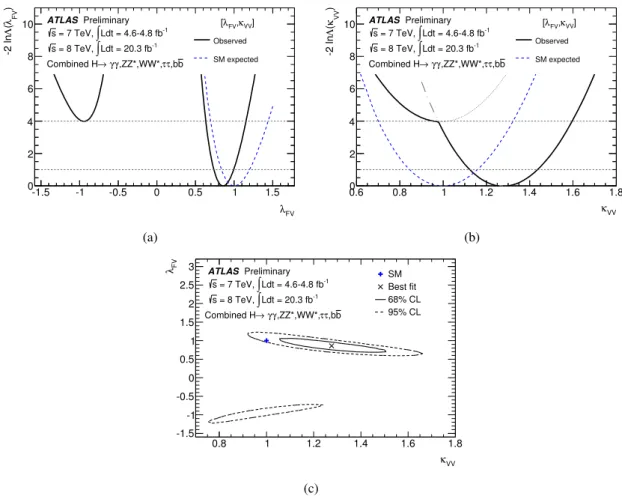
Figure 6 shows the results of this fit. The best-fit values and uncertainties, when profiling the other parameter, are:

λ

= 0.86

κ

= 1.28

.

Similarly to the above case, Figure 6(a) shows the determination of the sign of λ

. Figure 6(c) shows the two-dimensional likelihood contours. The two variables are anticorrelated because only their product appears in the model. The two-dimensional compatibility of the SM hypothesis with the best-fit point is 10%.

λFV

-1.5 -1 -0.5 0 0.5 1 1.5

) FVλ(Λ-2 ln

0 2 4 6 8

10 ^ATLASPreliminary Ldt = 4.6-4.8 fb-1

∫

= 7 TeV, s

Ldt = 20.3 fb-1

∫

= 8 TeV, s

b τ,b τ ,ZZ*,WW*, γ γ

→ Combined H

VV] ,κ λFV

[

Observed SM expected

(a)

κVV

0.6 0.8 1 1.2 1.4 1.6 1.8

)VVκ(Λ-2 ln

0 2 4 6 8

10 ^ATLAS Preliminary Ldt = 4.6-4.8 fb-1

∫

= 7 TeV, s

Ldt = 20.3 fb-1

∫

= 8 TeV, s

b τ,b τ ,ZZ*,WW*, γ γ

→ Combined H

VV] ,κ λFV

[

Observed SM expected

(b)

κVV

0.8 1 1.2 1.4 1.6 1.8

FVλ

-1.5 -1 -0.5 0 0.5 1 1.5 2 2.5

3 SM

Best fit 68% CL 95% CL ATLAS Preliminary

Ldt = 4.6-4.8 fb-1

∫

= 7 TeV, s

Ldt = 20.3 fb-1

∫

= 8 TeV, s

b τ,b ,ZZ*,WW*,τ γ γ Combined H→

(c)

Figure 6: Results of fits for the 2-parameter benchmark model defined in Section 5.2.2 that probe different coupling strength scale factors for fermions and vector bosons without assumptions on the total width:

(a) coupling scale factor ratio λ

( κ

is profiled); (b) coupling scale factor ratio κ

( λ

is profiled).

The dashed curves show the SM expectations. The thin dotted and dashed-dotted lines in (b) indicate the continuations of the likelihood curves when restricting the parameters to either the positive or negative sector of λ

; (c) correlation contours of the same variables.

5.2.3 Summary

The coupling of the new particle to fermions is observed directly in the H → ττ channel at more than 4σ [6], while the H → b b ¯ channel is compatible both with the SM Higgs boson and SM background.

This coupling is also observed indirectly through the constraints from the channels which are dominated

by the main production process gg → H, assumed to be fermion-mediated in this benchmark model.

The relatively large values of κ

in the first model and κ

in the second model reflect the large µ values measured for the bosonic modes.

5.3 Probing the custodial symmetry of the W and Z couplings

Identical coupling scale factors for the W and Z boson are required within tight bounds by the SU(2) custodial symmetry and the ρ parameter measurements at LEP and at the Tevatron [18]. To test this constraint directly in the Higgs sector, the ratio λ

= ^κ

/ κ

is probed. For the other parameters the same assumptions as in Section 5.2.1 on κ

are made ( κ

= ^κ

= ^κ

= ^κ

). The free parameters are:

λ

= ^κ

/ κ

λ

= ^κ

/ κ

κ

= ^κ

· κ

/ κ

. The relevant scaling formulae can be found in Appendix A.2.

The ratio λ

is in part directly constrained by the decays in the H→ WW

→ `ν`ν and H→ ZZ

→ 4`

channels and the W H and ZH production processes. It is also indirectly constrained by the VBF pro- duction process, which in the SM is 74% W fusion and 26% Z fusion-mediated (see Eq. 4). The scale factor κ

is also constrained by the H→ γγ channel since the decay branching ratio receives a dominant contribution from the W loop.

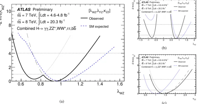
Figure 7 shows the likelihood functions for this benchmark scenario. There is a relative sign ambi- guity between the W and Z boson couplings. However, this relative sign is not accessible at the LHC

. The sign of λ

can be chosen positive without loss of generality.

The fit prefers the SM-like local minimum with a positive sign for λ

, implying a positive relative sign between the fermion and Z couplings, while the negative sign is still compatible at the ∼ 1σ level.

The minimum corresponding to negative λ

values is seen in Fig. 7(a) as the left branch of the observed and expected curves, and in Fig. 7(b).

The fit results for the parameters of interest, when profiling the other parameters, are:

λ

= 0.94

λ

∈ [−0.91, −0.63] ∪ [0.65, 1.00]

κ

= 1.41

.

The three-dimensional compatibility of the SM hypothesis with the best-fit point is 19%. In the diboson final state combination of Ref. [3], the minimum at negative λ

was disfavoured for the expectation, but the minima of the two branches were found to be similar for the data, due to the high value of the signal strength in the H→ γγ channel. With the addition of the direct fermion decay channels, the non-SM-like minimum is now also slightly disfavoured in the data.

In order to be independent of possible new physics contributions to the H→ γγ channel, the same analysis can be performed with an e ff ective coupling scale factor ratio λ

which is profiled in the mea- surement of λ

(see Ref. [3]). The measured value of λ

is in agreement with the expectation of custodial symmetry λ

= 1, regardless of the inclusion of the H→ γγ channel as an indirect constraint on κ

. With the availability of the direct fermion channels, this case is now covered by the generic model in Section 5.6.2, which yields consistent results.

6

In principle the VBF process has some sensitivity to the W and Z interference, but the interference term is << 1% and

hence too small to have any discriminating power.

λ

0.6 0.8 1 1.2 1.4 1.6

)

λ ( Λ -2 ln

0 2 4 6 8

10 ^ATLAS Preliminary Ldt = 4.6-4.8 fb

∫

= 7 TeV, s

Ldt = 20.3 fb

∫

= 8 TeV, s

b τ ,b τ ,ZZ*,WW*, γ

γ

→ Combined H

ZZ

] κ

FZ

, λ

WZ

, λ [

Observed SM expected

(a)

λFZ

-1.5 -1 -0.5 0 0.5 1 1.5 2

)FZλ(Λ-2 ln

0 2 4 6 8

10 ^ATLASPreliminary Ldt = 4.6-4.8 fb-1

∫

= 7 TeV, s

Ldt = 20.3 fb-1

∫

= 8 TeV, s

b τ,b τ ,ZZ*,WW*, γ γ

→ Combined H

ZZ] κ FZ, λ WZ, λ [ Observed SM expected

(b)

κZZ

0.5 1 1.5 2 2.5 3

)ZZκ(Λ-2 ln

0 2 4 6 8

10 ^ATLASPreliminary Ldt = 4.6-4.8 fb-1

∫

= 7 TeV, s

Ldt = 20.3 fb-1

∫

= 8 TeV, s

b τ,b τ ,ZZ*,WW*, γ γ

→ Combined H

ZZ] κ FZ, λ WZ, λ [ Observed SM expected

(c)

Figure 7: Results of fits for the benchmark model defined in Section 5.3 that probe the custodial sym- metry through the ratio λ

= ^κ

/ κ

: (a) coupling scale factor ratio λ

( λ

and κ

are profiled);

(b) coupling scale factor ratio λ

( λ

and κ

are profiled); (c) overall scale factor κ

( λ

and λ

are profiled). The dashed curves show the SM expectations. The thin dotted/dashed-dotted lines indi- cate the continuations of the likelihood curves when restricting the parameters to either the positive or negative sector of λ

.

5.4 Probing relations within the fermion coupling sector

The previous sections assumed universal coupling scale factors for all fermions, while many extensions of the SM predict deviations within the fermion sector. The currently accessible channels, in particular with the addition of H → b b ¯ and H → ττ, allow the relations between the up- and down-type fermion sector and between the lepton and quark sector to be probed.

5.4.1 Probing the up- and down-type fermion symmetry

Many extensions of the SM contain di ff erent couplings of the Higgs boson to up-type and down-type fermions. This is for instance the case for certain Two-Higgs-Doublet Models [14, 19–21], among which the MSSM is the most prominent example. In this model the ratio λ

between down- and up-type fermions is probed, while vector boson couplings are taken unified as κ

. The indices u, d stand for all up- and down-type fermions, respectively. The free parameters are:

λ

= ^κ

/ κ

λ

= κ

/ κ

κ

= ^κ

· κ

/ κ

. The relevant scaling formulae can be found in Appendix A.3.1.

The up-type quark coupling scale factor is mostly indirectly constrained through the gg → H pro-

duction channel, from the Higgs boson to top-quark coupling, while the down-type coupling strength is

constrained through the H → b b ¯ and H → ττ decays. Figure 8 shows the results for this benchmark

scenario. The likelihood curve is nearly symmetric about λ

= 0 as the model is almost insensitive to

the relative sign of κ

and κ

. The interference of contributions from the b and t loops in the gg → H production induces an asymmetry, much smaller than the present sensitivity (see Eq. 3). The fit results for the parameters of interest are:

λ

∈ [−1.24, −0.81] ∪ [0.78, 1.15]

λ

= 1.21

κ

= 0.86

.

The value of λ

around the SM-like minimum at 1 is λ

= 0.95

. This fit provides a ∼ 3.6σ level evidence of the coupling of the Higgs boson to down-type fermions, mostly coming from the H → ττ measurement. The three-dimensional compatibility of the SM hypothesis with the best-fit point is 20%.

λ

-2 -1.5 -1 -0.5 0 0.5 1 1.5 2

)

λ ( Λ -2 ln

0 2 4 6 8

10 ^ATLAS Preliminary Ldt = 4.6-4.8 fb

∫

= 7 TeV, s

Ldt = 20.3 fb

∫

= 8 TeV, s

b τ ,b τ ,ZZ*,WW*, γ

γ

→ Combined H

uu

] , κ λ

, [ λ

Observed SM expected

(a)

λVu

-2 -1.5 -1 -0.5 0 0.5 1 1.5 2

)Vuλ(Λ-2 ln

0 2 4 6 8

10 ^ATLASPreliminary Ldt = 4.6-4.8 fb-1

∫

= 7 TeV, s

Ldt = 20.3 fb-1

∫

= 8 TeV, s

b τ,b τ ,ZZ*,WW*, γ γ

→ Combined H

uu] κ du, λ Vu, λ [

Observed SM expected

(b)

κuu 0.4 0.6 0.8 1 1.2 1.4 1.6 1.8 2 )uuκ(Λ-2 ln

0 2 4 6 8

10 ^ATLASPreliminary Ldt = 4.6-4.8 fb-1

∫

= 7 TeV, s

Ldt = 20.3 fb-1

∫

= 8 TeV, s

b τ,b τ ,ZZ*,WW*, γ γ

→ Combined H

uu] κ du, λ Vu, λ [

Observed SM expected

(c)

Figure 8: Results of fits for the benchmark model described in Section 5.4.1 that probe the symmetry between down- and up-type fermions: (a) coupling scale factor ratio λ

( λ

and κ

are profiled);

(b) coupling scale factor ratio λ

( λ

and κ

are profiled); (c) overall scale factor κ

( λ

and λ

are profiled). The dashed curves show the SM expectations. The thin dotted / dashed-dotted lines indicate the continuations of the likelihood curves when restricting the parameters to either the positive or negative sector of λ

and λ

, respectively.

5.4.2 Probing the quark and lepton symmetry

Here the ratio λ

between leptons and quarks is probed, while vector boson couplings are taken unified as κ

. The indices l, q stand for all leptons and quarks, respectively. The free parameters are:

λ

= ^κ

/ κ

λ

= ^κ

/ κ

κ

= κ

· κ

/ κ

.

The relevant scaling formulae can be found in Appendix A.3.2. The lepton coupling strength is currently

only constrained through the H → ττ decay.

Figure 9 shows the results for this benchmark. Similar to the case above, the likelihood curve is nearly symmetric about λ

= 0 . The fit results for the parameters of interest are:

λ

∈ [−1.48, −0.99] ∪ [0.99, 1.50]

λ

= 1.27

κ

= 0.82

.

The value of λ

around the SM-like minimum at 1 is λ

= 1.22

. A vanishing coupling of the Higgs boson to leptons is excluded at the ∼ 4.0σ level due to the H → ττ measurement. The three-dimensional compatibility of the SM hypothesis with the best-fit point is 15%.

λ

-2 -1 0 1 2

)

λ ( Λ -2 ln

0 2 4 6 8

10 ^ATLAS Preliminary Ldt = 4.6-4.8 fb

∫

= 7 TeV, s

Ldt = 20.3 fb

∫

= 8 TeV, s

b τ ,b τ ,ZZ*,WW*, γ

γ

→ Combined H

qq

] κ

lq

, λ

Vq

, λ [

Observed SM expected

(a)

λVq

-2 -1.5 -1 -0.5 0 0.5 1 1.5 2

)Vqλ(Λ-2 ln

0 2 4 6 8

10 ^ATLASPreliminary Ldt = 4.6-4.8 fb-1

∫

= 7 TeV, s

Ldt = 20.3 fb-1

∫

= 8 TeV, s

b τ,b τ ,ZZ*,WW*, γ γ

→ Combined H

qq] κ lq, λ Vq, λ [ Observed SM expected

(b)

κqq 0.4 0.6 0.8 1 1.2 1.4 1.6 1.8 2 )qqκ(Λ-2 ln

0 2 4 6 8

10 ^ATLASPreliminary Ldt = 4.6-4.8 fb-1

∫

= 7 TeV, s

Ldt = 20.3 fb-1

∫

= 8 TeV, s

b τ,b τ ,ZZ*,WW*, γ γ

→ Combined H

qq] κ lq, λ Vq, λ [ Observed SM expected

(c)

Figure 9: Results of fits for the benchmark model described in Section 5.4.2 that probe the symmetry between quarks and leptons: (a) coupling scale factor ratio λ

( λ

and κ

are profiled); (b) coupling scale factor ratio λ

( λ

and κ

are profiled); (c) overall scale factor κ

( λ

and λ

are profiled). The dashed curves show the SM expectations. The thin dotted/dashed-dotted lines indicate the continuations of the likelihood curves when restricting the parameters to either the positive or negative sector of λ

and λ

, respectively.

5.5 Probing beyond the SM contributions

In this section contributions from new particles either in loops or in new final states are considered. All coupling scale factors of known SM particles are assumed to be as predicted by the SM, i.e. κ

= 1. For the H→ γγ and gg → H vertices, effective scale factors κ

and κ

are introduced that allow for extra contributions from new particles. The potential new particles contributing to the H→ γγ and gg → H loops may or may not contribute to the total width of the observed state through direct invisible decays or decays into final states that cannot be distinguished from the background. In these cases the resulting variation in the total width is parameterised in terms of the additional branching ratio into invisible or undetected particles BR

. Both aforementioned scenarios are addressed in this section.

7

Invisible final states can be directly searched for through the E

signature [22]. An example of an undetected mode

would be a decay mode to multiple light jets, which presently cannot be distinguished from multi-jet backgrounds.