Coupling properties of the new Higgs-like boson observed with the ATLAS detector at the LHC

ATLAS-CONF-2012-127 10/09/2012

ATLAS NOTE

ATLAS-CONF-2012-127

September 10, 2012

Coupling properties of the new Higgs-like boson observed with the ATLAS detector at the LHC

The ATLAS Collaboration

Abstract

Details of the production and decay of the new particle discovered in the mass region of 126 GeV in the search for the Standard Model Higgs boson at

s=

7 TeV and

s=

8 TeV are presented. The searches in the

4ℓ,

and

¯ channels include several exclusive final states, which provide sensitivity to the coupling properties of the observed particle through the various production and decay modes. Several benchmarks are considered that are designed to probe different aspects of the SM Higgs boson couplings. No significant deviation from the prediction for a SM Higgs boson is found.

c Copyright 2012 CERN for the benefit of the ATLAS Collaboration.

Reproduction of this article or parts of it is allowed as specified in the CC-BY-3.0 license.

1 Introduction

The observation of a new particle in the search for the Standard Model (SM) Higgs boson at the LHC reported by the ATLAS [1] and CMS [2] collaborations, is a milestone in the quest to understand electroweak symmetry breaking. In Ref. [1] the ATLAS collaboration reported the initial estimate for the mass of the particle to be

126.0

0.4 (stat)

0.4 (syst) GeV

obtained from the H

and H

ZZ

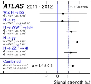
4ℓ channels. Figure 1 illustrates how this observation was made simultaneously in various SM Higgs boson search channels by showing the best fit value for the global signal strength

for a Higgs boson mass hypothesis of m

number of events from all combinations of production and decay modes relative to their SM values, for the individual channels and the combination. The signal strength parameter is a convenient observable to test the background-only hypothesis (µ

0) and the SM Higgs hypothesis (µ

1). However the detailed consistency of the production and decays of this new particle with the expectation for the SM Higgs boson still needed to be assessed.

µ) Signal strength ( -1 0 1 Combined

→ 4l ZZ(*)

→ H

γ γ

→ H

ν νl

→ l WW(*)

→ H

τ τ

→ H

→ bb W,Z H

Ldt = 4.6 - 4.8 fb-1

∫ = 7 TeV:

s

Ldt = 5.8 - 5.9 fb-1

∫ = 8 TeV:

s

Ldt = 4.8 fb-1

∫

= 7 TeV:

s

Ldt = 5.8 fb-1

∫

= 8 TeV:

s

Ldt = 4.8 fb-1

∫

= 7 TeV:

s

Ldt = 5.9 fb-1

∫

= 8 TeV:

s

Ldt = 4.7 fb-1

∫

= 7 TeV:

s

Ldt = 5.8 fb-1

∫

= 8 TeV:

s

Ldt = 4.7 fb-1

∫

= 7 TeV:

s

Ldt = 4.6-4.7 fb-1

∫

= 7 TeV:

s

= 126.0 GeV mH

± 0.3 = 1.4 µ

ATLAS

Figure 1: Measurements of the signal strength parameter

for m

and their combination.

This document presents the measurements of coupling properties of the observed new particle under several benchmark scenarios. The measured observables are deviations of the couplings from those predicted for a SM Higgs boson. The observed state is assumed to be a

-even scalar as the Higgs boson of the SM. The results are based on the same analyses and data sets as in Ref. [1] with the same statistical model describing the experimental and theoretical systematic uncertainties. The aspects of the individual channels relevant for these measurements are summarized in Section 2. Section 3 outlines the statistical procedures used for considering multi-parameter likelihood functions. The systematic uncertainties that contribute to the measurements are listed in Section 4. Model-independent contours in terms of production cross-sections and branching ratios are presented in Section 5. Finally, the results of fits to specific benchmarks designed to probe Higgs boson couplings are presented in Section 6.

The benchmarks follow the recommendations of the LHC Higgs Cross Section Working Group [3] and

references therein, in particular the approach adopted in this note was initiated in Refs. [4, 5, 6, 7, 8, 9] .

2 Individual Channels

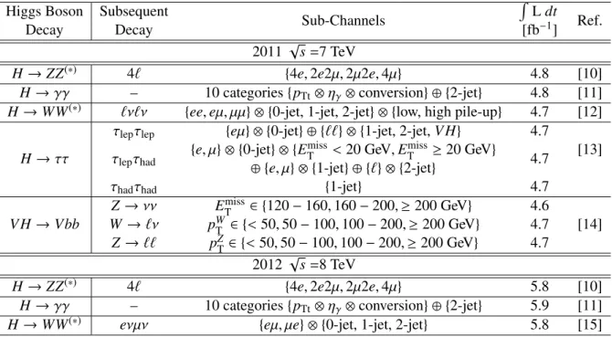
The different channel categories considered in this analysis are summarized in Table 1. Many of the sub-channels are introduced to enhance sensitivity to the SM Higgs boson (e.g., the categorization of events according to lepton flavor or low/high pile-up) but do not provide any discrimination between different production modes. In contrast, requirements on lepton and jet multiplicities, on low/high-p

(a variable related to the transverse momentum of the Higgs boson) in the H

channel, and on E

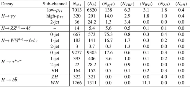
(the transverse missing momentum) provide discrimination between different production modes. Table 2 summarizes the primary sources of discrimination between the different production modes and provides representative numbers of events satisfying the selection requirements from the various SM production modes for a 126 GeV Higgs boson. These numbers refer to mass windows that contain about 90% of the signal and to the combination of the luminosities and centre-of-mass energies reported in Table 1.

Table 1: Summary of the individual channels entering the combination. The transition points between separately optimized m

regions are indicated where applicable. In channels sensitive to associated production of the Higgs boson, V indicates a W or Z boson. The symbols

and

represent direct products and sums over sets of selection requirements, respectively.

Higgs Boson Subsequent

Sub-Channels

R

L dt

Decay Decay [fb

] Ref.

2011

s

H

ZZ

4ℓ

4e, 2e2µ, 2µ2e, 4µ

4.8 [10]

H

– 10 categories

p

conversion

2-jet

4.8 [11]

H

WW

ee, eµ, µµ

0-jet, 1-jet, 2-jet

low, high pile-up

4.7 [12]

H

τ_lepτ_lep {

eµ

0-jet

1-jet, 2-jet, V H

4.7

τ_lepτ_had {

e, µ

0-jet

E

20 GeV, E

20 GeV

4.7 [13]

⊕ {

e, µ

1-jet

2-jet

τ_hadτ_had {

1-jet

4.7

V H

Vbb

Z

E

120

160, 160

200,

200 GeV

4.6

W

p

50, 50

100, 100

200,

200 GeV

4.7 [14]

Z

p

50, 50

100, 100

200,

200 GeV

4.7 2012

s

H

ZZ

4ℓ

4e, 2e2µ, 2µ2e, 4µ

5.8 [10]

H

– 10 categories

p

conversion

2-jet

5.9 [11]

H

WW

eνµν

eµ, µe

0-jet, 1-jet, 2-jet

5.8 [15]

3 Statistical Procedure

The statistical modeling of the data is described in Refs. [16, 17, 18, 19, 20]. For each production mode i, a signal strength factor

defined by

is introduced. Similarly, for each decay final state, f , a factor

B

is introduced. For each analysis category (k) the number of signal events (n

) is parametrized as:

n







 X

i

µ_iσ_i,SM×

A







×µ_f ×

B

(1)

Table 2: Summary of the number of selected events, background and expected SM signal contributions for a 126 GeV Higgs boson, estimated in invariant or transverse mass intervals containing

90% of the signal around the most probable value of the invariant or transverse mass distributions, from various production modes satisfying all selection requirements. These numbers refer to the combination of the luminosities and centre-of-mass energies reported in Table 1. Categories that do not provide significant discrimination between production modes are merged.

Decay Sub-channel N

N

N

N

N

N

N

H

low-p

7013 6820 138 6.3 3.1 1.8 0.4

high-p

320 291 14.0 2.9 1.8 1.0 0.4

2-jet 36 24.2 1.3 3.4 0.0 0.0 0.0

H

ZZ

4ℓ – 14 5.4 5.6 0.5 0.1 0.1 0.0

H

WW

0-jet 667 573 75.3 0.8 0.3 0.4 0.0

1-jet 183 141 16.7 1.7 0.3 0.2 0.0

2-jet 3 3.7 0.3 1.3 0.0 0.0 0.0

H

0-jet 9277 9305 17.6 0.6 0.1 0.3 0.0

1-jet 393 406 3.6 1.0 0.1 0.2 0.0

2-jet 22 28.2 0.3 0.9 0.0 0.0 0.0

VH 164 152 0.7 0.1 0.2 0.3 0.0

H

b b ¯ ZH 322 321 0.0 0.0 0.0 4.0 0.0

W H 1266 1311 0.0 0.0 11.1 0.0 0.0

where A represents the detector acceptance,

the reconstruction efficiency and

the integrated luminos- ity. The number of signal events expected from each combination of production and decay is scaled by the corresponding product of

, with no change to the distribution of kinematic or other properties

. This parametrization generalizes the dependency of the signal yields on the production cross sections and decay branching fractions, allowing for a coherent variation across several channels. This approach is also general in the sense that it is not restricted by any relationship between production cross sections and branching ratios. For instance, it is possible to force the production cross section

0 while maintaining a positive branching ratio B

. The relationship between production and decay in the con- text of a specific theory or benchmark is achieved via a parametrization of

f (κ), where the

are the parameters of the theory or benchmark under consideration as defined in Section 6.

Given the observed data, the resulting likelihood function is a function of a vector of signal strength factors

are tested with a statistic

the profile likelihood ratio [21].

Λ(µ)=

L

ˆˆ

L( ˆ

ˆ (2)

where the single circumflex denotes the unconditional maximum likelihood estimate of a parameter and the double circumflex (e.g.

ˆˆ of

given fixed values of

the full likelihood function. When the signal strength parameters

are reparametrized in terms of

1Occasionally the productµiµfis also represented by a single signal strength parameterµj, where jis an index representing both the production and decay indicesiandf. For example, the global signal strengthµin Figure 1 is used for all combinations of production and decay.

2HereΛis used for the profile likelihood ratio to avoid confusion with the parameterλused in the benchmarks.

the same equation is used for

with a Higgs boson mass hypothesis fixed to its measured value of m

Higgs boson mass hypothesis to float, using it as an additional nuisance parameter, and thus taking into account the experimental uncertainty on its estimate, were performed and no significant deviations from the results presented herein were observed.

Given the achieved experimental precision on the mass determination from the H

and H

ZZ

4ℓ channels, that is at the 4 per mil level, its value has been fixed to the measured value of m

126 GeV in all coupling measurements reported in Section 6.

Asymptotically, the test statistic

2 ln

) is distributed as a

distribution with n degrees of free- dom, where n is the dimensionality of the vector

. In particular, the 100(1

contours are defined by

2 ln

)

k

, where k

satisfies P(χ

k

)

the 68% and 95% CL contours are given by

2 ln

)

2.3 and 6.0, respectively.

4 Systematic Uncertainties

The treatment of systematic uncertainties and their correlations is described in detail in Ref. [22]. Sys- tematic uncertainties on observables are handled by introducing nuisance parameters with a probability density function (pdf) associated with the estimate of the correspondent systematic. These nuisance parameters, in particular those representing instrumental uncertainties or background estimates, are of- ten assessed from auxiliary measurements, such as control regions, sidebands, or dedicated calibration measurements. Their pdf is then well described either by a Gaussian or alternatively by a log-normal distribution to avoid the truncation of a pdf bounded to a restricted range. In cases where the uncertainty is related to a number of events (e.g. from Monte Carlo or data control samples) the gamma function can be used. However, for nuisance parameters unconstrained by considerations or measurements, a pdf is not a priori defined. This is typically the case for theory uncertainties on the prediction of produc- tion cross sections or branching ratios. The natural choice for such uncertainties is a rectangular pdf.

However, due to the discontinuities in its definition, this choice also causes unwanted fit instabilities. In this note, theory systematic uncertainties are treated using the less conceptually appropriate but better behaved log-normal pdf. For these specific theory uncertainties, the difference with respect to simple variations have shown that the effect of this choice does not alter the conclusions of this note. Alternative choices are currently under study.

Theoretical uncertainties are important to quantify the consistency of the observation with the SM expectation, and are therefore included. Particularly relevant in the measurement of coupling proper- ties of the observed state are the theoretical uncertainties on the signal cross sections and exclusive jet multiplicity requirements. The prescription used follows the recommendations of Refs. [23, 24], treat- ing these systematic uncertainties as fully correlated across channels. Similarly, the H

channel takes into account migration between the categories due to uncertainty in the p

distribution from the gluon-fusion and vector boson fusion processes. Theoretical uncertainties associated with the branching ratios are small in comparison to both experimental uncertainties and the uncertainty in the production cross sections. Uncertainties in the acceptance due to parton density functions and renormalization and factorization scale choices are included.

5 Production Signal Strength in Individual Decay Modes

Before fits to Higgs boson coupling parameters are presented in the next section, this section focuses on

the measured signal strength in different final states: the signal strengths of different Higgs production

processes contributing to the same final state are separated. This avoids the complications of a consis-

tent parametrization of both production and decay mode modifications caused by potential beyond-SM effects.

In the SM, the production cross sections are completely fixed once m

is specified. However, the best fit value for the global signal strength factor

does not give any direct information on the relative contributions from different production modes. Furthermore, fixing the ratios of the production cross sections to the ratios predicted by the SM may conceal tension between the data and the SM.

In order to address any tension between the data and the ratios of production cross sections predicted in the SM, the individual channels must separate the signal contribution from various production modes.

A test of the SM combining multiple decay modes is complicated by the fact that the underlying cou- plings between the Higgs and other particles affect both the production and the decay. Furthermore, parametrization of these effects is subject to a number of assumptions on the presence or absence of new particle states in loop-induced couplings and unobserved decay modes affecting the total width of the Higgs boson.

Since several Higgs boson production modes are available at the LHC, results shown in two dimen- sional plots require either some

to be fixed or several

to be related. No direct ttH production has been observed yet, hence

and the very small contribution of

have been grouped together as they scale dominantly with the ttH coupling in the SM and are denoted by the common parameter

. Similarly,

and

have been grouped together as they scale with the W H/ZH gauge coupling in the SM and are denoted by the common parameter

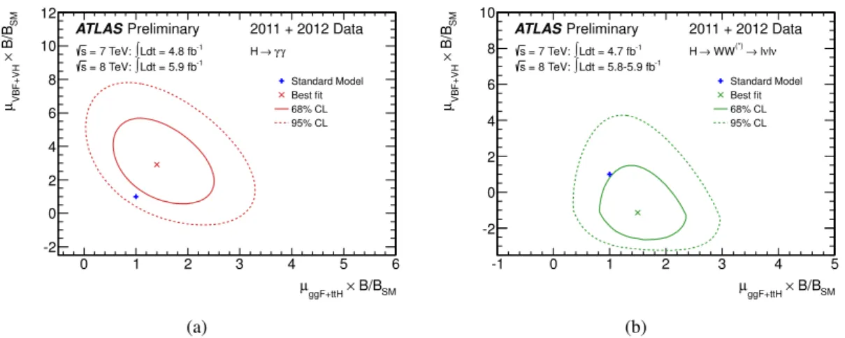
. The resulting contours for the H

and H

WW

channels at m

derived varying only the

parameters of Equation 1 and the

parameters are fixed to unity. These factors are not constrained to positive values only, in order to accomodate downward fluctuations of the background; similarly to the procedure of Ref. [16] where the global strength parameter is allowed to be negative. For the H

ZZ

4ℓ channel only the inclusive analysis has been performed due to the lim- ited statistical power of this channel. It should be noted that the factors

in different decay modes could have different values, hence a direct comparison of the results among different final states is not possible.

Such comparisons need consistent coupling modifications in the initial state the and final state, as dis- cussed in the next section. It is nevertheless possible using their ratio to eliminate the dependence on the branching fraction and illustrate the relative discriminating power between

ttH and V BF

V H , as well as the compatibility of the measurements in each channel. The likelihood as a function of the ratio

for the H

and H

WW

channels and their combination is shown in Fig. 3.

6 Coupling Properties Measurements

Following the framework and benchmarks as recommended by Ref. [25], measurements of coupling scale factors are implemented using a lowest-order-motivated framework. This framework makes the following assumptions:

•

Only modifications of couplings strengths, i.e. of absolute values of couplings, are taken into account: the observed state is assumed to be a

-even scalar as in the SM.

•

The signals observed in the different search channels originate from a single narrow resonance with a mass of 126 GeV. The case of several, possibly overlapping, resonances in this mass region is not considered.

•

The width of the Higgs boson with a mass of 126 GeV is assumed to be negligible. Hence the

B/BSM ggF+ttH× µ

0 1 2 3 4 5 6

SM B/B×VBF+VHµ

-2 0 2 4 6 8 10 12

γ γ

→ H

Standard Model Best fit 68% CL 95% CL

Preliminary ATLAS

Ldt = 4.8 fb-1

∫ = 7 TeV:

s

Ldt = 5.9 fb-1

∫ = 8 TeV:

s

2011 + 2012 Data

(a)

B/BSM ggF+ttH× µ

-1 0 1 2 3 4 5

SM B/B×VBF+VHµ

-2 0 2 4 6 8 10

ν νl

→ l WW(*)

→ H

Standard Model Best fit 68% CL 95% CL

Preliminary ATLAS

Ldt = 4.7 fb-1

∫ = 7 TeV:

s

Ldt = 5.8-5.9 fb-1

∫ = 8 TeV:

s

2011 + 2012 Data

(b)

Figure 2: Likelihood contours for the H

and H

WW

channels in the (µ

) plane including the branching ratio factor B/B

. The quantity

(µ

) is a common scale factor for the ggF and t¯ tH (VBF and V H) production cross sections (the

parameters in Equation 1 are fixed). The best fit to the data (

) and 68% (full) and 95% (dashed) CL contours are also indicated, as well as the SM expectation (+).

ggF+ttH

µ

VBF+VH / µ

-3 -2 -1 0 1 2 3 4 5 6

Λ-2 ln

0 1 2 3 4 5 6 7 8 9

ν νl

→ l WW(*)

→ and H γ γ

→ H

γ γ

→ H

ν νl

→ l WW(*)

→ H

Preliminary ATLAS

Ldt = 4.7-4.8 fb-1

∫ = 7 TeV:

s

Ldt = 5.8-5.9 fb-1

∫ = 8 TeV:

s

2011 + 2012 Data

Figure 3: Likelihood curves for

from the H

and H

WW

channels and their combination. The branching ratios cancel in this ratio so that the curves can be compared.

product

BR(ii

H

) can be decomposed in the following way for all channels:

σ×

BR(ii

H

)

Γ_H

(3)

where

is the production cross section through the initial state ii,

the partial decay width into the final state

and

the total width of the Higgs boson.

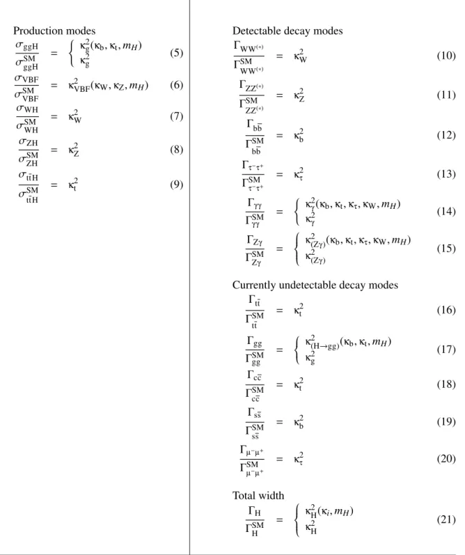
The leading order (LO) motivated scale factors

are defined in such a way that the cross sections

and the partial decay widths

associated with the SM particle i scale with the factor

when compared to the corresponding SM prediction. Table 3 lists all relevant cases. Taking the process gg

H

as an example, one would use as cross section:

(σ

BR) (gg

H

)

(gg

H)

BR

(H

)

2g·^κ2γ

κ_H²

(4)

where the values and uncertainties for both

(gg

H) and BR

(H

) are taken from Refs. [23, 24, 26] for a given Higgs boson mass hypothesis.

The simplest model assumes that all couplings are modified by a single scaling parameter

. In this case the fit to the data yields a value of

κ=

1.19

0.11 (stat)

0.03 (syst)

0.06 (theory) corresponding to the square root of the global signal strength

shown in Figure 1.

More refined benchmark models to probe the couplings of the observed Higgs-like particle have been elaborated in Ref. [3], and references therein, to address specific questions on its nature, under various assumptions. These assumptions will change depending on the question being discussed.

In the forthcoming subsections the following fundamental questions related to the coupling properties are addressed. The relative couplings to fermions and bosons are tested in Section 6.1, assuming two common scale factor for these two sectors. The ratio of couplings to W and Z bosons, related to the custodial symmetry, is discussed in Section 6.2.1 . The ratio of down to up quark type couplings, that is very interesting for several extensions of the SM, is discussed in Section 6.2.2. The ratio of couplings to the lepton and quark sectors is given in Section 6.2.3. The possible effect of beyond SM particles on the indirect coupling to gluons and photons, that in the SM proceeds via loops and therefore is particularly sensitive the new physics, is given in Section 6.3.

The main results discussed herein are compared with the results expected from the presence of a m

6.1 Couplings to Fermions and Vector Gauge Bosons

This benchmark is an extension of the single parameter

fit, where a different strength for the fermion and vector coupling is probed. It assumes that only SM particles contribute to the H

and

H vertex loops. The fit is performed in two variants, with and without the assumption that the total width of the Higgs boson is given by the sum of the known SM Higgs boson decay modes (modified in strength by the appropriate fermion and vector coupling scale factors).

6.1.1 Assuming only SM particles contribute to the total width

The fit parameters are the coupling scale factors

for all fermions and

for all vector couplings:

κ_F = κ_t =κ_b =κτ

(22)

κ_V = κW =κZ

(23)

Figure 4(a) shows the result of the fit to this benchmark. Only the relative sign between

and

is physical and some sensitivity to this sign is gained from the negative interference between the W-loop and t-loop in the H

decay. The fit gives a small preference to the local minimum close the SM point. The likelihood as a function of

when

is profiled and as a function of

when

is profiled is illustrated in Figure 5(a) and Figure 5(b) respectively. Figure 5(a) shows in particular to what extent the sign degeneracy is resolved.

The 68% CL intervals of

and

when profiling over all other parameters are:

κ_F ∈

[

1.0,

0.7]

[0.7, 1.3] (24)

κ_V ∈

[0.9, 1.0]

[1.1, 1.3] (25)

These intervals combine all experimental and theoretical systematic uncertainties. The 95% confidence intervals are

κ_F ∈

[

1.5,

0.5]

[0.5, 1.7] (26)

κV ∈

[0.7, 1.4] (27)

Production modes

σ^SM_ggH = ( _κ2

g

(

m

)

κ²_g

(5)

σ_VBF

σ^SM_VBF = κ²_VBF

(

m

) (6)

σ^SM_WH = κ²_W

(7)

σ_ZH

σ^SM_ZH = κ²_Z

(8)

σ_{tt H} σ^SM

tt H

= κ²_t

(9)

Detectable decay modes

Γ^SM

WW^(∗)

= κ²_W

(10)

Γ_ZZ(∗)

Γ^SM

ZZ^(∗)

= κ²_Z

(11)

Γ_bb Γ^SM

bb

= κ²_b

(12)

Γτ−τ⁺

Γ^SM_τ−τ+

= κ²_τ

(13)

Γγγ

Γ^SM_γγ = ( _κ2

γ

(

m

)

κ²_γ

(14)

Γ_Zγ Γ^SM_Zγ =











κ²_(Zγ)

(

m

)

κ²_(Zγ)

(15)

Currently undetectable decay modes

Γ^SM

tt

= κ²_t

(16)

Γ_gg Γ^SM_gg =







κ²_(H→gg)

(

m

)

κ²_g

(17)

Γ_cc

Γ^SM_cc = κ²_t

(18)

Γ_ss Γ^SM

ss

= κ²_b

(19)

Γ_µ−µ⁺

Γ^SM_µ−µ+

= κ²_τ

(20)

Total width











κ²_H

(

m

)

κ²_H

(21)

Table 3: Leading order (LO) coupling scale factor relations for Higgs boson cross sections and partial decay widths relative to the SM as defined in Ref. [25]. For a given m

hypothesis, the smallest set of degrees of freedom in this framework comprises

,

,

,

, and

. For partial widths that are not detectable at the LHC, scaling is performed via proxies chosen among the detectable ones. Additionally, the loop-induced vertices can be treated as a function of other

or effectively, through the

and

degrees of freedom which allow probing for BSM contributions in the loops. Finally, to explore invisible

or undetectable decays, the scaling of the total width can also be taken as a separate degree of freedom,

, instead of being rescaled as a function,

(

), of the other scale factors.

κV

0.4 0.6 0.8 1 1.2 1.4 1.6 1.8

Fκ

-2 -1 0 1 2 3 4

SM Best fit

) < 2.3 κF V, κ Λ( -2 ln

) < 6.0 κF V, κ Λ( -2 ln Ldt = 5.8-5.9 fb-1

∫

= 8TeV, s

Ldt = 4.8 fb-1

∫

= 7TeV, s

ATLASPreliminary

(a)

κVV

0 0.5 1 1.5 2 2.5

FVλ

-2 -1 0

1 2 3 4

SM Best fit

) < 2.3 λFV VV, κ Λ( -2 ln

) < 6.0 λFV VV, κ Λ( -2 ln Ldt = 5.8-5.9 fb-1

∫

= 8TeV, s

Ldt = 4.8 fb-1

∫

= 7TeV, s

ATLASPreliminary

(b)

Figure 4: Fits for 2-parameter benchmark models probing different coupling strength scale factors for fermions and vector bosons: (a) Correlation of the coupling scale factors

and

, assuming no non- SM contribution to the total width; (b) Correlation of the coupling scale factors

and

without assumptions on the total width.

The confidence intervals on

and

are reduced by approximately 20% when removing all theoretical systematic uncertainties and further reduced by approximately 5% when removing the experimental systematic uncertainties on the signal. The (2D) compatibility of the SM hypothesis with the best fit point is 21%.

6.1.2 Relaxing the assumption on the total width

Without the assumption on the total width, only ratios of coupling scale factors can be measured. Hence there are now the following free parameters:

λFV = κF/κV

(28)

κVV = κV ·^κV/κH

(29)

λ_FV

is the ratio of the fermion and vector coupling scale factors, and

an overall scale that includes the total width and applies to all rates. Figure 4(b) shows the results of this fit. The 68% confidence interval of

when profiling over

yields:

λFV ∈

[

1.1,

0.7]

[0.6, 1.1] (30)

(31) The 95% confidence intervals are:

λ_FV ∈

[

1.8,

0.5]

[0.5, 1.5] (32)

(33) The confidence interval on

is reduced by approximately 10% when removing all theoretical system- atic uncertainties and further reduced by 10% when removing the experimental systematic uncertainties on the signal. The (2D) compatibility of the SM hypothesis with the best fit point is 21%. It should be noted that the assumption on the total width gives a strong constraint on the fermion coupling scale factor

, since it is dominated in the SM by the b-decay width. The measurement of

, profiling the

parameter yields:

1.2

−0.6

.

κF

-2 -1.5 -1 -0.5 0 0.5 1 1.5 2

)Fκ(Λ-2 ln

0 1 2 3 4 5 6 7 8

F) κ Λ( -2 ln Ldt = 5.8-5.9 fb-1

∫

= 8TeV, s

Ldt = 4.8 fb-1

∫

= 7TeV, s

ATLASPreliminary

(a)

κV

0.6 0.8 1 1.2 1.4 1.6

) Vκ(Λ-2 ln

0 1 2 3 4 5 6

7 )

κV

Λ( -2 ln Ldt = 5.8-5.9 fb-1

∫

= 8TeV, s

Ldt = 4.8 fb-1

∫

= 7TeV, s

ATLASPreliminary

(b)

Figure 5: Fits for benchmark models probing different coupling strength scale factor for fermions and vector bosons, assuming no non-SM contribution to the total width: (a) coupling scale factor for fermions

(the coupling scale factor for gauge bosons

is profiled) and (b) coupling scale factor for gauge bosons

(the coupling scale factor for fermions

is profiled).

6.1.3 Conclusions

The non-vanishing value of the fitted coupling of the new particle to gauge bosons

is both directly and indirectly constrained by several channels. The coupling to fermions is directly observed in the H

and H

b b ¯ channels, the direct constraint is therefore very weak as no significant deviation from SM expectations is observed in these channels. A value of

significantly deviating from zero is indirectly observed through the constraints from both the channels which are dominated by the main production

H process and those aimed at selecting the VBF production process.

6.2 Probing the Structure of Fermion and Vector Couplings

Both previous benchmarks assume that the coupling scale factors for the W- and Z-boson are identical (

) and that the scale factors for all fermions are identical (

). In the following subsections both assumptions are relaxed and tested. Since this test is focused on coupling ratios the assumption on the total width has been relaxed.

6.2.1 Probing the custodial symmetry of the W and Z coupling

Identical coupling scale factors for the W- and Z-boson are required within tight bounds by SU(2)

custodial symmetry and the

parameter measurements at LEP [27]. To test this directly in the Higgs sector, the ratio

is probed. Otherwise the same assumptions as in Section 6.1.2 on

are made (

). The free parameters are:

κZZ = κZ·^κZ/κH

(34)

λWZ = κW/κZ

(35)

λ_FZ = κ_F/κ_Z

(36)

Figure 6(a) shows the likelihood distribution for the interesting ratio

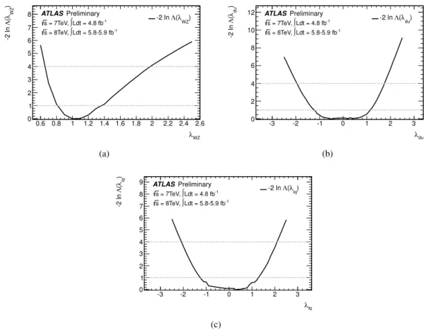
. The measurement of

, when profiling the

and

observables is:

λWZ =

1.07

(37)

λWZ

0.6 0.8 1 1.2 1.4 1.6 1.8 2 2.2 2.4 2.6 )WZλ(Λ-2 ln

0 1 2 3 4 5 6 7

8 )

λWZ

Λ( -2 ln Ldt = 5.8-5.9 fb-1

∫

= 8TeV, s

Ldt = 4.8 fb-1

∫

= 7TeV, s

ATLASPreliminary

(a)

λdu

-3 -2 -1 0 1 2 3

)duλ(Λ-2 ln

0 2 4 6 8 10

12 )

λdu

Λ( -2 ln Ldt = 5.8-5.9 fb-1

∫

= 8TeV, s

Ldt = 4.8 fb-1

∫

= 7TeV, s

ATLASPreliminary

(b)

λlq

-3 -2 -1 0 1 2 3

)lqλ(Λ-2 ln

0 1 2 3 4 5 6 7 8 9

lq) λ Λ( -2 ln Ldt = 5.8-5.9 fb-1

∫

= 8TeV, s

Ldt = 4.8 fb-1

∫

= 7TeV, s

ATLASPreliminary

(c)

Figure 6: Fits for benchmark models probing for deviations within the vector or fermion sector: (a) prob- ing the ratio

; (b) probing the ratio

; (c) probing the ratio

.

In the measurement of the ratio

the theoretical and experimental systematic uncertainties have a very small effect. The (3D) compatibility of the SM hypothesis with the best fit point is 33%. Fits to the two additional parameters of the model yields

1.3

and

[

1.1,

0.5]

[0.6, 1.2] at 68% CL.

6.2.2 Probing the up- and down-type fermion symmetry

In many extensions of the SM the couplings of the light Higgs boson to up-type and down-type fermions differ. The ratio

between down- and up-type fermions is probed with the same assumptions as in Section 6.1.2 on

(

); then

and

. The free parameters are:

κ_uu = κ_u·^κu/κ_H

(38)

λ_du = κ_d/κ_u

(39)

λ_Vu = κ_V/κ_u

(40)

Figure 6(b) shows the likelihood distribution for the ratio

. The 68% CL interval of

when profiling the

and

observables is:

λ_du ∈

[

1.2, 1.2] (41)

at 68% CL. The 95% confidence interval is

λdu ∈

[

2.0, 1.8] (42)

The range in the measurement of

is dominated by the low sensitivity in the H

and H

b b ¯ channels, therefore removing the theoretical and experimental systematic uncertainties has a very small effect. The (3D) compatibility of the SM hypothesis with the best fit point is 33%. Fits to the additional parameters yield

1.0

and

[

1.3,

1.1]

[0.8, 1.6] at 68% CL.

6.2.3 Probing the quark and lepton symmetry

Here the ratio

between leptons and quarks is probed. The same assumptions as in Section 6.1.2 are made on

(

); then

and

. The free parameters are:

κqq = κq·^κq/κH

(43)

λ_lq = κ_l/κ_q

(44)

λ_Vq = κ_V/κ_q

(45)

Figure 6(c) shows the likelihood distribution for the ratio

. The 68% CL interval of

when profiling the

and

observables is:

λ_lq ∈

[

1.3, 1.3] (46)

at 68% CL. The 95% confidence intervals is

λ_lq ∈

[

2.1, 2.1] (47)

The range in

is dominated by the low sensitivity in the H

channel, therefore removing the theoretical and experimental systematic uncertainties has a very small effect. The (3D) compatibility of the SM hypothesis with the best fit point is 31%. Fits to the additional parameters yield:

1.0

and

1.1

.

6.2.4 Conclusions

The ratio

probes the custodial symmetry through the relative coupling of the new particle to the W and Z bosons. The fit of

is in part directly constrained by the direct decays in the H

WW

and H

ZZ

4ℓ channels. The

part is also indirectly constrained by the H

channel since the decay branching ratio gets a dominant contribution from

. The measured value of

is in agreement, within the uncertainties (which are at present dominated by statistical uncertainties) with the custodial symmetry, as expected for a SM Higgs boson.

The uncertainty on the measurement of relative strength of the coupling of the observed state to the up- and down-type fermions is dominated by the measurement of its decay in the H

and H

b b ¯ channels. The ratio (

) is therefore only weakly constrained by the current data. Similarly the

ratio mainly relies on the H

channel and therefore is only weakly constrained.

6.3 Probing Potential Non-SM Particle Contributions

This case allows for new particle contributions either in loops or in new final states. All coupling scale factors of known SM particles are as in the SM, i.e.

1. For the H

and

H vertices, effective scale factors

and

are introduced. They allow for extra contributions from new particles.

The potential new particles contributing to the H

and

H loops, may or may not contribute to

the total width of the observed state from direct invisible decays or decays into event topologies that are

not distinct from the background. In the latter case the resulting variation in total width is parameterized

in terms of the additional branching ratio BR

. The two aforementioned cases are addressed in

this section.

κγ

0.6 0.8 1 1.2 1.4 1.6 1.8 2 2.2

gκ

0.5 1 1.5 2

2.5 SM

Best fit ) < 2.3 κg γ, κ Λ( -2 ln

) < 6.0 κg γ, κ Λ( -2 ln Ldt = 5.8-5.9 fb-1

∫

= 8TeV, s

Ldt = 4.8 fb-1

∫

= 7TeV, s

ATLASPreliminary

(a)

inv.,undet.

BR 0 0.1 0.2 0.3 0.4 0.5 0.6 0.7 0.8 0.9 )inv.,undet.(BRΛ-2 ln

0 1 2 3 4 5 6

7 )

inv.,undet.

Λ(BR -2 ln Ldt = 5.8-5.9 fb-1

∫

= 8TeV, s

Ldt = 4.8 fb-1

∫

= 7TeV, s

ATLASPreliminary

(b)

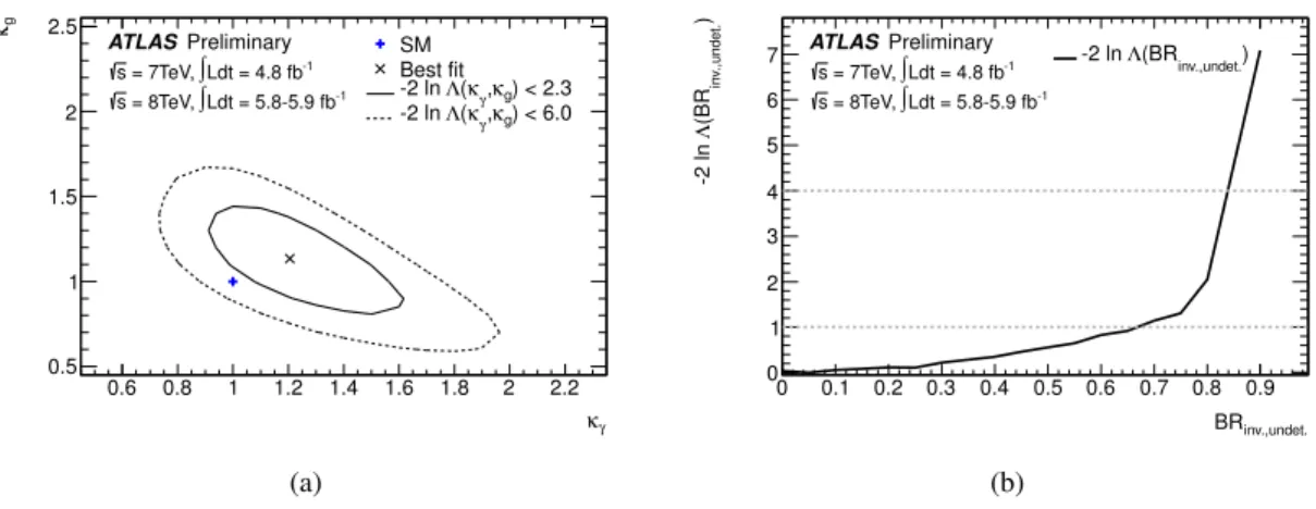
Figure 7: Fits for benchmark models probing for contributions from non-SM particles: (a) Probing only the

H and H

loops, assuming no sizable extra contribution to the total width; (b) Probing in addition to (a) for a possible invisible or undetectable branching ratio BR

.

6.3.1 Assuming only SM particles contributing to the total width

A fit is shown in Figure 7(a) which assumes that there are no sizeable extra contributions to the total width caused by the non-SM particles. The free parameters are

and

.

Figure 7(a) shows the 68% and 95% CL contours for the two parameters. The best fit values and uncertainties when profiling over the other parameter are

κ_g =

1.1

(48)

κγ =

1.2

(49)

at 68% CL. When removing the theoretical systematic uncertainties on the measurements of

and

, the uncertainty is reduced by O(15 %). It is further reduced by O(5%) when removing the experimental systematic uncertainties. The compatibility of the SM hypothesis (2D) with the best fit point is 18%.

6.3.2 No assumption on the total width

By constraining some of the factors to be equal to their SM values, it is possible to probe for new non-SM decay modes that might appear as invisible or undetectable final states. The free parameters are

,

and BR

. In this model the modification to the total width is parametrized as follows:

Γ_H =

κ²_H

(

)

(1

BR

)

(50)

Figure 7(b) shows the likelihood as a function of BR

when

and

are profiled. The best fit values and uncertainties, and confidence level interval at 68% CL when profiling over the other parameters are

κ_g =

1.1

(51)

κγ =

1.2

(52)

BR

0.68 (53)

The 95% confidence level interval on the invisible or undetectable branching fraction is BR

0.84. The 68% CL interval for the invisible or undetectable branching fraction without theory systematic

uncertainties (on signal) is BR

0.62. Without all experimental systematic uncertainties, the 68% CL confidence interval further reduces to BR

0.57. The (3D) compatibility of the SM hypothesis with the best fit point is 35%.

6.3.3 Conclusions

In the hypothesis where all couplings of the new particle to Standard Model particles are fixed to the values of the Standard Model Higgs boson and in the absence of additional contributions to the total width, and within the statistics of the present data, no significant deviation is observed in the effective coupling to photons and gluons (

and

respectively). Releasing the assumption on the total width mildly constrains BR

, favoring small values.

7 Conclusion

Using data taken in 2011 and 2012, at centre-of-mass energies of respectively 7 TeV and 8 TeV and cor- responding altogether to approximately 10 fb

, the ATLAS collaboration has reported the observation of a new particle with a mass of m

126.0

0.4(stat)

0.4(syst) GeV, in the search for the Standard Model Higgs boson. The same data set was further analysed to investigate the coupling properties of the new observed particle. Simplified benchmark models were used to study the correlations of production and decay modes in different final states, and compare them to the predictions for the SM Higgs boson.

Within the current statistical uncertainties and assumptions, no significant deviations from the Standard

Model couplings are observed.