ATLAS-CONF-2012-091 07July2012
ATLAS NOTE
ATLAS-CONF-2012-091
July 6, 2012
Observation of an excess of events in the search for the Standard Model Higgs boson in the γγ channel with the ATLAS detector
The ATLAS Collaboration
Abstract
This note reports on a search for the Standard Model Higgs boson in the diphoton decay channel in proton-proton collisions at center-of-mass energies of √
s = 7 TeV and √ s = 8 TeV using integrated luminosities of 4.8 fb−1and 5.9 fb−1, respectively, recorded with the ATLAS detector at the Large Hadron Collider. The search is performed for Higgs boson masses between 110 and 150 GeV.
The expected exclusion limit at 95% confidence level varies between 0.8 and 1.6 times the Standard Model cross section over the studied mass range, and results in an expected exclusion range from 110 GeV to 139.5 GeV. The observed exclusion ranges for a Stan- dard Model Higgs boson are found to be (112−122.5) GeV and (132−143) GeV at 95%
confidence level.
In between the two excluded regions, an excess of events is observed around the diphoton system invariant mass of about 126.5 GeV with a local significance of 4.5σ.
c Copyright 2012 CERN for the benefit of the ATLAS Collaboration.
Reproduction of this article or parts of it is allowed as specified in the CC-BY-3.0 license.
1 Introduction
The search for the Higgs boson [1–3], which is closely tied to the mechanism of electroweak symmetry breaking in the Standard Model (SM), as well as in many models beyond the SM, is one of the key mis- sions of the Large Hadron Collider (LHC) at CERN. The LEP experiments have excluded the existence of a SM Higgs boson with a mass smaller than 114.4 GeV at 95% confidence level [4]. Recent results of the experiments operated at the Tevatron collider exclude at 95% confidence level a SM Higgs boson in the range from 100 GeV to 106 GeV and from 147 GeV to 179 GeV at 95% confidence level [5]. Searches by the ATLAS experiment have narrowed the allowed range for a SM Higgs boson to be between 117.5 GeV and 118.5 GeV, between 122.5 GeV and 129 GeV and above 539 GeV [6], and from the CMS experiment the allowed range is below 127.5 GeV and above 600 GeV [7], where the excluded regions are excluded at 95% confidence level. The search for the Higgs boson decay to two photons strongly contributes to the Higgs boson search in the low mass range, m
H <150 GeV [8, 9]. In the data sample acquired during 2011, ATLAS finds a deviation from the background-only hypothesis at an invariant diphoton mass of 126.5 GeV which corresponds to a local significance of 2.8σ, while the largest deviation reported by CMS corresponds to 3.1σ local significance at a diphoton invariant mass of 124 GeV.
This note presents the analysis strategy and the results of the search for the SM Higgs boson in the diphoton decay channel with the full data sample acquired in 2011, corresponding to 4.8 fb
−1at
√
s
=7 TeV, and the first 5.9 fb
−1of integrated luminosity recorded in 2012 at
√s
=8 TeV, with the ATLAS detector at the LHC at CERN. The analysis largely follows the previous analysis of the
√
s
=7 TeV data [8], but with substantial improvements. The event categorization has been re-optimized by introducing a category enriched in vector-boson fusion production candidates, which requires an improved selection of the primary vertex associated to the hard interaction. The parametrization of the shape of background distributions has been reconsidered in order to further limit potential biases. A new photon isolation variable has also been adopted, which is less affected by multiple collisions occurring in the same or neighboring bunch crossings, a phenomenon known as “pileup”. In addition, a neural- network based photon identification is used for the
√s
=7 TeV data. For the
√s
=8 TeV data, a converted photon reconstruction and cut-based photon identification have been introduced which are less sensitive to pileup. Due to the different center-of-mass energies during 2011 and 2012, the two data samples are analyzed separately, and the results are combined statistically.
The note is organized as follows. Sec. 2 introduces the ATLAS detector. Sec. 3 describes the photon reconstruction and the event selection. The categorization of events is detailed in Sec. 4. Sec. 5 contains a discussion of the background modeling, as well as the breakdown of the selected sample into its different components. Sec. 6 summarizes the modeling of the signal decays. Finally, Sec. 7 presents the results of the search.
2 The ATLAS detector and data sample
The ATLAS detector [10] consists of an inner tracking detector surrounded by a superconducting solenoid providing a 2 T magnetic field, electromagnetic and hadron calorimeters, and a muon spectrometer. The main sub-detectors relevant to the search presented here are the calorimeters, in particular the electro- magnetic section, and the inner tracking system. The inner detector provides tracking in the pseudora- pidity
1region
|η|<2.5 and consists of silicon pixel- and microstrip-detectors inside a transition radiation
1ATLAS uses a right-handed coordinate system with its origin at the nominal interaction point (IP) in the center of the detector and thez-axis along the beam line. thex-axis points from the IP to the center of the LHC ring, and they-axis points upwards. Cylindrical coordinates (r, φ) are used in the transverse plane,φbeing the azimuthal angle around the beam line.
The pseudorapidity is defined in terms of the polar angleθasη=−ln tanθ2. Transverse momentum and energy are defined as pT =psinθandET=Esinθ, respectively.
tracker. The tracking detectors consist of a barrel part and two end-cap sections. The transition radiation tracker provides electron identification through transition radiation in scintillating foils and fibers. The electromagnetic calorimeter, a lead/liquid-argon sampling device, is divided in one barrel (
|η| <1.475) and two end-cap (1.375
< |η| <3.2) sections. Longitudinally, it is divided into three layers. The first layer, referred to as the strip layer, has a fine segmentation in
ηto facilitate the separation of photons from neutral hadrons and to allow the measurement of the shower direction. Most of the energy is deposited in the second layer, and the third layer serves for the correction of the energy deposited downstream of the electromagnetic calorimeter. In the range of
|η| <1.8 a presampler layer inside the cryostat allows for the correction of energy losses upstream of the calorimeter. The barrel (
|η| <0.8) and extended barrel (0.8
< |η| <1.7) hadron calorimeter sections consist of steel and scintillating tiles, while the end-cap sections (1.5
< |η| <3.2) are composed of copper and liquid argon. The forward calorimeter (3.1
<|η|<4.9) uses copper and tungsten as absorber with liquid argon as active material.
After the application of data-quality requirements, the data samples amount to 4.8 fb
−1at
√s
=7 TeV and 5.9 fb
−1at
√s
=8 TeV, respectively. The data were recorded with instantaneous luminosity varying between 1
×10
32cm
−2s
−1and 6.8
×10
33cm
−2s
−1. The mean number of interactions per bunch crossing has a mean of 9.1 in the data sample acquired during 2011, and of 19.5 for the data taken up to June 2012. The simulation is corrected to reflect the distribution of interactions per bunch crossing and the spread of the z position of the primary vertex observed in data.
The data sample considered in this analysis was selected using a diphoton trigger. In the last step of the triggering chain, two clusters formed from energy depositions in the electromagnetic calorimeter are required. A transverse energy threshold of 20 GeV is required on both clusters for the
√s
=7 TeV run, while for the
√s
=8 TeV data sample, the thresholds are increased to 35 GeV and 25 GeV on the leading (most energetic) and subleading (next most energetic) clusters, respectively. In addition, loose criteria are applied on the shapes of the electromagnetic clusters to require them to match the expectations for electromagnetic showers initiated by photons. The trigger has an efficiency greater than 99% for events passing the final event selection.
3 Photon reconstruction and selection of H → γγ candidates
3.1 Photon reconstruction and identification
The photon reconstruction is seeded from clusters of energy deposits in the electromagnetic calorime- ter. The reconstruction is designed to separate electrons, unconverted photons, and converted photons, which arise from conversions of photons in the detector material to electron-positron pairs. The clusters are matched to tracks and to conversion vertex candidates, which have been reconstructed in the inner detector and extrapolated to the second layer of the calorimeter [11]. Clusters without any matching track or conversion vertex are classified as unconverted photon candidates. Clusters with a matching vertex reconstructed from one or two tracks are converted photon candidates. For the reconstruction of the
√s
=8 TeV data, the tracking, vertexing and the matching to clusters have been improved to ensure that the reconstruction of converted photons is robust against pileup. The efficiency of the new photon reconstruction is about 96.5% averaged over the transverse momentum p
Tand
ηspectra expected for photons from a Higgs boson decay.
The energies of the clusters are calibrated, separately for unconverted and converted candidates, to
account for energy losses upstream of the calorimeter and for energy leakage outside of the cluster. The
calibration is refined by applying
η-dependent correction factors, which are of the order of±1%, deter-
mined from Z
→e
+e
−events. In addition, the energy measurement of converted photons is improved
with corrections based on dedicated Monte Carlo simulation (MC) studies. The simulation is corrected
to reflect the energy resolution observed using Z
→e
+e
−events in data, which requires an energy smear-
ing of about 1% in the calorimeter barrel region and between 1.2% and up to 2.1% in the calorimeter end-caps. From these studies, the uncertainty on the constant term of the energy resolution is about 50%, while the uncertainty on the energy resolution ranges between 5% and 20% for electrons with
p
T∼60 GeV, depending on the region of the calorimeter [12].
The identification of photons is based on shower shapes measured in the electromagnetic calorimeter.
An initial loose cut-based selection, used also at trigger level, is based on shower shapes in the second layer of the electromagnetic calorimeter, as well as the energy deposition in the hadronic calorimeter.
A tight identification adds information from the finely segmented strip layer of the calorimeter, which provides good rejection of hadronic jets where a neutral meson carries most of the jet energy. The shower shape values in the simulation are shifted slightly to improve the agreement with the data shower shapes. Two variants of the tight photon identification are used. For the
√s
=7 TeV data, a neural- network based selection, tuned to achieve similar jet rejection as the cut-based menu used in [8] but with higher efficiency, is used. For the
√s
=8 TeV data, due to the necessity of ensuring a reliable photon performance for data recorded very recently, a cut-based selection is used, which has been tuned for robustness against pileup effects by relaxing requirements on shower shapes more susceptible to pileup, and tightening others. The photon identification efficiencies, averaged over
η, range between 85% andabove 95% for the p
Trange considered for a Higgs boson with mass as low as m
H=120 GeV.
To further suppress hadronic background, an isolation requirement is applied. The isolation trans- verse energy is estimated by summing the transverse energy of positive-energy topological clusters
2reconstructed in the electromagnetic and hadronic calorimeters in a cone of
∆R=0.4 around the photon candidate, where the region within 0.125
×0.175 in
η×φaround the photon barycenter is excluded.
The isolation is corrected for leakage of the photon energy outside of the excluded region. The positive- energy topological clusters are also used as an input to a low- p
Tjet algorithm using k
Tclustering [14,15].
From low-p
Tjets, the ambient energy in the event from pileup as well as the underlying event is calcu- lated and used to correct the photon isolation event-by-event (for more details see [16] and references therein).
The distribution of the isolation variable has been studied in data and simulation using electrons from Z
→e
+e
−events, and photons from Z
→e
+e
−γevents. The data and simulation have been found to be in good agreement and the remaining small discrepancy is accounted for as a systematic uncertainty. In the following, photon candidates are required to have an isolation transverse energy of less than 4 GeV.
3.2 Event and candidate selection
Events are selected by the diphoton trigger and are required to contain at least two reconstructed photon candidates in the fiducial region of the calorimeter,
|η| <1.37 or 1.52
< |η| <2.37. The barrel-endcap transition regions, 1.37
< |η| <1.52 are excluded. To ensure well-reconstructed photon candidates, further quality requirements are applied to the reconstructed clusters. Similarly, converted photon candi- dates reconstructed from tracks passing through dead modules of the innermost pixel layer are rejected, strongly decreasing the misidentification of electrons as converted photons. Further criteria are applied to the two highest-p
Tphoton candidates. The leading photon candidate is required to have p
T >40 GeV, and the subleading photon candidate p
T >30 GeV. Tight identification criteria as detailed in Sec. 3.1 are applied to both photon candidates. Furthermore, both photon candidates are required to be isolated in the calorimeter.
With this selection, 23788 diphoton candidates are observed in the diphoton invariant mass range between 100 and 160 GeV in the
√s
=7 TeV data sample. In the same mass range, 35271 events are selected in the
√s
=8 TeV data sample.
2Topological clusters are three-dimensional clusters of variable size, built by associating calorimeter cells on the basis of the signal-to-noise ratio [13].
[GeV]
γ
mγ
116 118 120 122 124 126 128 130 132 134 / 0.5 GeVγγ1/N dN/dm
0 0.02 0.04 0.06 0.08 0.1
0.12 True vertex
2
pT
Σ Max Likelihood Calo pointing
ATLAS Simulation Preliminary
γ γ
→
→ H gg
= 125 GeV mH
= 8 TeV s
Number of reconstructed primary vertices
0 5 10 15 20 25 30
Efficiency
0 0.2 0.4 0.6 0.8 1
2
pT
Σ PV with max PV from likelihood
MC signal (Gluon fusion + VBF)
=125 GeV = 8 TeV, mH
s
ATLAS Simulation Preliminary
Figure 1: Left: distribution of the expected diphoton mass for H
→ γγsignal events as a function of the algorithm used to determine the longitudinal vertex position of the hard-scattering event. The use of the calorimeter information, labelled as ”Calo pointing” is fully adequate to reach the optimal achievable mass resolution labelled as ”True vertex”. The likelihood described in the text, combining this information with the primary vertex information from the tracking, provides similar mass resolution.
Right: the dependence of the efficiency for selecting a reconstructed primary vertex within
∆z=0.2 mm of the true hard interaction vertex using two different methods: the highest
Pp
2Tof all tracks assigned to a vertex (black) and from the likelihood as described in the text (blue). The addition of the tracking information from the inner detector is necessary to improve the efficiency of identification of the hard- interaction primary vertex needed for the jet selection.
3.3 Trigger e ffi ciency
The efficiency of the trigger for events passing the analysis selection is determined by a bootstrap ap- proach: the efficiency of the trigger selection with respect to offline photons is factorized as the high-level trigger selection efficiency relative to the Level-1 seed, multiplied by the Level-1 seed efficiency. These efficiencies are evaluated from unbiased events, as described in [17].
The efficiency of the diphoton trigger used for the
√s
=7 TeV data is measured to be (98.9
±0.2)%. The efficiency of the diphoton trigger for the
√s
=8 TeV data is found to be (99.6
±0.1)%. No dependence on pileup is observed on
√s
=8 TeV data for loose photon triggers up to 25 primary vertices per event. To estimate the systematic uncertainty due to the method and to the unknown composition of the data sample, the efficiency of the loose diphoton trigger was also evaluated using a tag and probe method on Z
→e
+e
−γdata events when one of the electrons radiates a photon, using a simulated H
→γγsample and from simulated events containing jets misidentified as photons. The difference with respect to the efficiency computed with the bootstrap approach results in a systematic uncertainty of less than 1%.
3.4 Primary vertex selection and estimation of the diphoton invariant mass
The selection of the primary vertex is relevant for two aspects of the analysis: the estimation of the invariant mass of the diphoton system, and the selection of the jets associated with the hard interaction, as described in Sec. 4. While the former only has requirements on the resolution of the primary vertex position, the latter requires the identification of a specific vertex.
The primary vertex of the hard interaction is identified by combining the following elements in a
global likelihood: the directions of flight of the photons as determined by the measurements using the
longitudinal segmentation of the calorimeter, the average beam spot position, and the
Pp
2Tof the tracks associated with each reconstructed vertex. In case of the
√s
=7 TeV data, the conversion vertex is also used in the likelihood for converted photons with tracks containing silicon hits. As shown in Fig. 1 (left), the calorimeter information (with a resolution of
σz ∼15 mm using only the calorimeter pointing, and
σz ∼6 mm for two converted photons with silicon hits, if the vertex information is used) is sufficient to improve the mass resolution and is very close to the optimal resolution that can be achieved by using the true hard scattering primary vertex position. The mass resolution is similar when the likelihood is used to select the primary vertex. The addition of the tracking information from the inner detector is necessary to improve the identification of the hard-interaction primary vertex needed for the jet selection. Fig. 1 (left) shows the efficiency of finding the correct primary vertex as a function of the number of reconstructed vertices in the event using different methods. The decrease of the efficiency of finding the correct hard interaction primary vertex at high pileup can lead to an inefficiency in identifying the jets that accompany the Higgs boson production.
The invariant mass of the two photons is then estimated using the photon energies as measured in the calorimeter,
φas determined from the position of the photon in the calorimeter, and
ηas determined by the identified primary vertex and the photon impact point in the calorimeter.
4 Jet reconstruction and event categorization
Classifying events into subsamples with different signal-to-background ratios and different invariant mass resolutions improves the sensitivity of the search [18]. Multiple event properties are used for the catego- rization:
•
the
ηregion of the two photons in the calorimeter,
•
whether the photon candidates are converted or unconverted,
•
the p
Tt[19,20] of the diphoton system. The p
Ttof the diphoton system is defined as the orthogonal component of the diphoton momentum when projected on the axis ˆ t given by the difference of the photon momenta
~p
γ1Tand
~p
γ2T. Thus, p
Tt = |(
~p
γ1T +~p
γ2T)
×t ˆ
|, where ˆ t
=(~ p
γ1T −~p
γ2T)/
|~p
γ1T − ~p
γ2T |. Events with p
Tt<60 GeV form the low-p
Ttsample, while the remaining events form the high-p
Ttsample.
•
whether an event passes the 2-jets selection with a vector-boson fusion-like signature, described in Sec. 4.1.
The variable p
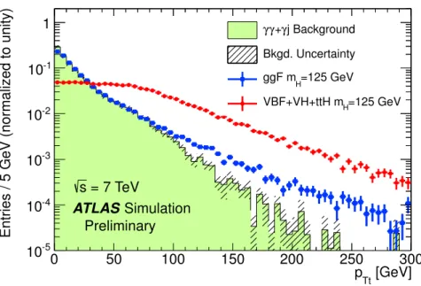
Ttis strongly correlated with the diphoton transverse momentum, but it has a better detector resolution and retains a monotonically falling diphoton invariant mass distribution for the back- ground events in the search region given the chosen cut values (see below). The latter quality is advan- tageous for the background modeling and associated uncertainties discussed below. The p
Ttdistribution in simulated background events and in simulated Higgs boson events is shown in Fig. 2 normalized to the same area. The background is obtained from SM
γγMC simulated with SHERPA [21] and
γ-jet MCsimulated with ALPGEN [22]. The two contributions have been normalized to their respective fractions observed on data (see Sec. 5), while the small jet-jet and Drell-Yan components have been neglected.
Fig. 2 also shows the difference in the p
Ttdistribution for different Higgs boson production processes, which can serve for their separation in addition to jet-based selections.
4.1 2-Jets selection
The dominant SM Higgs boson production process is gluon fusion. The second-most prominent produc-
tion process is vector-boson fusion (VBF). The VBF signature consists of two forward jets, with little
[GeV]
pTt
0 50 100 150 200 250 300
Entries / 5 GeV (normalized to unity)
10-5
10-4
10-3
10-2
10-1
1 γγ+γj Background
Bkgd. Uncertainty
=125 GeV ggF mH
=125 GeV VBF+VH+ttH mH
ATLAS Simulation Preliminary
= 7 TeV s
Figure 2: Distribution of p
Ttin simulated events with Higgs boson production and in background events.
The signal distribution is shown separately for gluon fusion (blue), and vector-boson fusion together with associated production (red). The background MC samples are described in the text. The background MC and the two signal distributions are normalized to unit area.
QCD radiation in the central region from the hard interaction.
Jets are reconstructed using the anti-k
talgorithm [23] with distance parameter R
=0.4. The inputs to the jet finding are three-dimensional topological calorimeter clusters [13, 24, 25] taken at the electro- magnetic (EM) scale. The jets are calibrated in three steps. First, the dependence of the jet response to the number of primary vertices and the average number of interactions is removed by applying a pileup correction derived from simulated samples [26]. Second, a jet origin correction [25] that adjusts the direction of the jet such that it points back to the primary vertex identified as the one with the highest
Pp
2Tof the associated tracks is applied. Finally, a MC-derived energy and pseudorapidity dependent correction [25] is applied. For the
√s
=7 TeV data, residual data-driven calibrations are derived using various in situ techniques that exploit the transverse momentum balance between a jet and a reference object, and are applied to the jet four-momenta [27].
A subsample of the data is enriched in VBF events by applying the following 2-jets selection:
•
The event must have at least two hadronic jets with
ηjet
<
4.5 and p
jetT >25 GeV. For the
√
s
=8 TeV analysis, the p
jetTcut is raised to 30 GeV for jets with 2.5
<|η|<4.5. Jets in the tracker acceptance range (
|η| <2.5) are required to have a jet-vertex-fraction of at least 0.75. The jet- vertex-fraction is defined as the fraction of the sum of p
Tcarried by tracks in the jet and associated to the primary vertex selected with the likelihood method with respect to the total p
Tcarried by all the tracks associated to the jet. The jets are required to pass jet quality cuts and to have a minimum distance
∆R =0.4 to any of the selected photons. Among the selected jets, the two jets with the highest p
Tare considered as the tagging jets.
•
The pseudorapidity gap between the tagging jets,
∆ηj j, has to be larger than 2.8.
•
The invariant mass of the tagging jets, m
j j, has to be larger than 400 GeV.
•
The azimuthal angle difference
∆φbetween the diphoton system and the system of the two tagging jets has to be larger than 2.6.
For simulated VBF events, the efficiency of the 2-jets selection is 29% for the
√s
=7 TeV analysis and 24% for the
√s
=8 TeV analysis.
The fraction of selected diphoton data events that pass the 2-jets selection is found to depend only weakly on the number of reconstructed primary vertices.
4.2 Event categories
As explained above, the event sample is split into exclusive categories. Events passing the 2-jets selection are excluded from the other categories.
1. Unconverted central, low p
Tt: Both photon candidates are reconstructed as unconverted photons and have
|η|<0.75. The diphoton system has low p
Tt.
2. Unconverted central, high p
Tt: Both photon candidates are reconstructed as unconverted photons and have
|η|<0.75. The diphoton system has high p
Tt.
3. Unconverted rest, low p
Tt: Both photon candidates are reconstructed as unconverted photons and at least one candidate has
|η|>0.75. The diphoton system has low p
Tt.
4. Unconverted rest, high p
Tt: Both photon candidates are reconstructed as unconverted photons and at least one candidate has
|η|>0.75. The diphoton system has high p
Tt.
5. Converted central, low p
Tt: At least one photon candidate is reconstructed as converted photon and both photon candidates have
|η|<0.75. The diphoton system has low p
Tt.
6. Converted central, high p
Tt: At least one photon candidate is reconstructed as converted photon and both photon candidates have
|η|<0.75. The diphoton system has high p
Tt.
7. Converted rest, low p
Tt: At least one photon candidate is reconstructed as a converted photon and both photon candidates have
|η|<1.3 or
|η|>1.75, but at least one photon candidate has
|η|>0.75.
The diphoton system has low p
Tt.
8. Converted rest, high p
Tt: At least one photon candidate is reconstructed as a converted photon and both photon candidates have
|η|<1.3 or
|η|>1.75, but at least one photon candidate has
|η|>0.75.
The diphoton system has high p
Tt.
9. Converted transition: At least one photon candidate is reconstructed as a converted photon and at least one photon candidate is in the range 1.3
<|η|<1.37 or 1.52
<|η|<1.75.
10. 2-jets: The event passes the 2-jets selection to enrich in VBF final states as described in Sec. 4.1.
The number of events observed in the different categories in the diphoton invariant mass range be- tween 100 and 160 GeV for the analyzed datasets is given in Table 1. In addition, the data sample is studied without categorization. This is referred to as the inclusive sample.
The contribution of each category to the analysis depends on its mass resolution, its signal-to- background ratio and its statistical power. Table 2 shows the expected number of signal and background events at
√s
=8 TeV and their ratio in a window around m
H =126.5 GeV that would contain 90% of
the signal events, along with the observed number of events in this window. The number of background
events has been obtained from a fit to the invariant mass distribution as described in Sec. 5. Table 2 is
representative of the sensitivity to a Higgs boson signal with a mass in the region of (120
−130) GeV.
Table 1: Number of events observed in the different categories in 4.8 fb
−1of
√s
=7 TeV data and 5.9 fb
−1of
√s
=8 TeV data in the diphoton invariant mass range between 100 GeV and 160 GeV.
Category
√s
=7 TeV data [N
evt]
√s
=8 TeV data [N
evt]
Unconverted central, low p
Tt2054 2945
Unconverted central, high p
Tt97 173
Unconverted rest, low p
Tt7129 12136
Unconverted rest, high p
Tt444 785
Converted central, low p
Tt1493 2021
Converted central, high p
Tt77 113
Converted rest, low p
Tt8313 11112
Converted rest, high p
Tt501 708
Converted transition 3591 5149
2-jets 89 129
Total 23788 35271
The FWHM and the resolution of the expected signal as discussed in Sec. 6 are also given. The “central”
categories, where both photons pass through the region with less material in front of the calorimeter, show the best invariant mass resolution, while it is lower for categories with photons reconstructed in other regions of the calorimeter.
5 Background composition and modeling
5.1 Background composition
The main processes contributing to the background in the H
→γγsearch can be divided into two classes:
the irreducible background consisting of QCD diphoton production, and the reducible background con- sisting of associated production of a photon with jets and processes with several jets in the final state.
The last two contribute to the background when one or two jets fragmenting into neutral mesons (mainly
π0) are misidentified as prompt photons. Understanding the composition of the selected sample serves as a monitoring of the performance of the photon identification, as well as a validation of the description of the backgrounds to the H
→γγsearch in the simulation. The latter is an important ingredient to the choice of the background parametrization, where also the sample composition determined from data is used.
Several methods based on varying photon identification and isolation criteria are used to determine the composition of the diphoton candidate events [28, 29]. They yield consistent results within their uncertainties. The fraction of diphoton events in the selected sample has been estimated to be (80
±4)%
in the
√s
=7 TeV data and (75
+3−2)% in the
√s
=8 TeV data. The fraction of
γ-jet and jet-jet events hasbeen found to be (19
±3)% ((22
±2)%) and (1.8
±0.5)% ((2.6
±0.5)%) in the
√s
=7(8) TeV data sample.
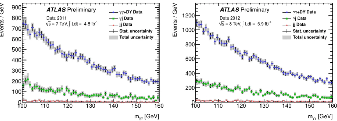
Fig. 3 shows the composition of the diphoton invariant mass spectrum, presented in bins of 1 GeV.
Background from Drell-Yan processes arises through the mis-reconstruction of electrons as photons, mostly through reconstruction of electrons as converted photons. Electrons from Drell-Yan processes have an isolation profile similar to that of signal photons. The misidentification rates are measured by using Z
→e
+e
−data events reconstructed as dielectron and e-γ pairs. For the
√s
=7 TeV data, the Drell- Yan background in the mass region (100
−160) GeV is estimated to be N
γγDY =325
±3(stat)
±30(syst).
For the
√s
=8 TeV data, the Drell-Yan background in the region (100
−160) GeV is estimated to be
Table 2: Number of expected signal S and background events B in mass a window around m
H =126.5 GeV that would contain 90% of the expected signal events, along with the observed number of events in this window. In addition,
σCB, the Gaussian width of the Crystal Ball function describing the invariant mass distribution (see Sec. 6), and the FWHM of the distribution, are given. The numbers are given for the data and simulation at
√s
=8 TeV for different categories and the inclusive sample.
Category
σCBFWHM Observed S B
[GeV] [GeV] [N
evt] [N
evt] [N
evt]
Inclusive 1.63 3.87 3693 100.4 3635
Unconverted central, low p
Tt1.45 3.42 235 13.0 215 Unconverted central, high p
Tt1.37 3.23 15 2.3 14 Unconverted rest, low p
Tt1.57 3.72 1131 28.3 1133
Unconverted rest, high p
Tt1.51 3.55 75 4.8 68
Converted central, low p
Tt1.67 3.94 208 8.2 193
Converted central, high p
Tt1.50 3.54 13 1.5 10
Converted rest, low p
Tt1.93 4.54 1350 24.6 1346
Converted rest, high p
Tt1.68 3.96 69 4.1 72
Converted transition 2.65 6.24 880 11.7 845
2-jets 1.57 3.70 18 2.6 12
N
γγDY =270
±4(stat)
±24(syst). The lower level of Drell-Yan background in the
√s
=8 TeV data is due to the improvements in the reconstruction of converted photons. The background from Drell-Yan processes is located in the low invariant mass region as can be seen in Fig. 4 for the
√s
=8 TeV sample and is very small in the invariant mass region used in this analysis.
5.2 Background modeling
For statistical analysis of the measured diphoton spectrum, the background is parametrized by an an- alytic function for each category, where the normalization and the shape are obtained from fits to the diphoton invariant mass distribution. Different parametrizations are chosen for the different event cat- egories to achieve a good compromise between limiting the size of a potential bias introduced by the chosen parametrization and retaining good statistical power. Depending on the category, an exponential function, a fourth-order Bernstein polynomial or an exponential function of a second-order polynomial is used (see Table 3). For the analysis of the inclusive sample, a fourth-order Bernstein polynomial is used.
Potential biases from the choice of background parametrization are estimated using three different sets of high statistics background-only MC models. The prompt diphoton background is obtained from the three generators RESBOS [30], DIPHOX [31], and SHERPA [21], while the same reducible back- ground samples are used for all three models. These are based on SHERPA for the
γ-jet backgroundand on PYTHIA6 [32] for the jet-jet background. Detector effects are included in some samples with with weighting and smearing techniques. In the SHERPA and PYTHIA samples, detector effects are taken into account, including photon identification efficiency, photon energy resolution, the process of photons being faked by jets, and the fraction of converted photons in the different detector regions. In the RESBOS and DIPHOX samples, the effect of photon identification efficiency is taken into account.
In addition, the Drell-Yan background component is taken into account; the shape and number of events
for this background is extracted from data-driven studies (see above). Each of these MC models is mixed
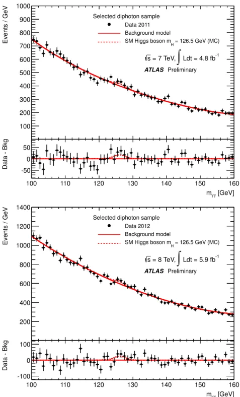
[GeV]
γ
mγ
100 110 120 130 140 150 160
Events / GeV
0 100 200 300 400 500 600 700 800
900 γγ+DY Data
j Data γ jj Data Stat. uncertainty Total uncertainty
ATLASPreliminary
Ldt = 4.8 fb-1
∫
= 7 TeV, s Data 2011
[GeV]
γ
mγ
100 110 120 130 140 150 160
Events / GeV
0 200 400 600 800 1000
1200 γγγj Data+DY Data
jj Data Stat. uncertainty Total uncertainty
ATLASPreliminary
Ldt = 5.9 fb-1
∫
= 8 TeV, s Data 2012
Figure 3: Diphoton sample composition as a function of the invariant mass for the
√s
=7 TeV (left) and the
√s
=8 TeV (right) dataset. The small contribution from Drell-Yan events is included in the diphoton component.
from the different components in the proportions estimated from data and is normalized to the total number of events observed in the data.
A variety of functional forms are considered for the background parametrization: single and double exponential functions, Bernstein polynomials up to seventh order, exponentials of second and third- order polynomials, and exponentials with modified turn-on behavior. The potential bias for a given parametrization is estimated by performing a maximum likelihood fit in the mass range of (100
−160) GeV using the sum of a signal and the background parametrization to all three sets of background- only simulation models for each category. The signal shape is taken to follow the expectation for an SM Higgs (see Sec. 6) in terms of shape, with a mass between 110 GeV and 150 GeV, and with the normalization floating. The categories mainly affected by background parametrization bias are the high- statistics categories, which also have a lower signal to background ratio. Parametrizations that exhibit problems with fit convergence are discarded. Parametrizations for which the estimated potential bias is smaller than 20% of the uncertainty on the fitted signal yield, or where the bias is smaller than 10%
of the number of expected signal events for each of the background models are selected for further studies. Among these selected parametrizations, the parametrization with the best expected sensitivity at m
H =125 GeV is selected as the background parametrization. For categories with low statistics, an exponential function is found to have sufficiently small bias, while polynomials and exponentials of poly- nomials, respectively, are needed for limiting the potential bias to stay within the predefined requirements for the higher-statistics categories.
For the chosen parametrization, the largest observed absolute signal yield over the full mass range studied (from 110 GeV to 150 GeV) is used as the potential bias for a given category, using the back- ground model based on SHERPA for the diphoton component. The selected parametrizations along with their potential bias, which is taken as an estimate of the systematic uncertainty due to the choice of parametrization, are shown in Table 3.
The invariant mass distributions and their composition obtained from the high-statistics simulation
model based on SHERPA for the diphoton component have been cross checked against data in different
categories, using the same background decomposition method as used for the inclusive sample (see
Sec. 5.1). Within the statistical uncertainties of data, a good agreement is found for the shapes of the
invariant mass distributions. The invariant mass distributions of the different categories have also been
compared with invariant mass distributions in a signal-depleted sample based on reversal of the photon
isolation selection. After accounting for the different sample composition in the isolation signal and
[GeV]
γ
m
γ70 80 90 100 110 120 130 140 150 160
Events / GeV
1 10 10
210
310
410
5ATLAS Preliminary
L dt=5.9 fb-1
∫
= 8 TeV, s
Data 2012
γ γ
→ee Z
Figure 4: Invariant mass distribution after applying the diphoton selection: Data (black) and estimated contribution of Z
→e
+e
−events to the diphoton invariant mass distribution (green) for the
√s
=8 TeV sample. This background contribution is obtained from reconstructed Z
→e
+e
−events in data.
sideband regions, a good agreement of the invariant mass distributions is found.
6 Signal modeling
The modeling of the signal, both in terms of Higgs boson production, and of detector response to a H
→γγsignal, is essential to set upper limits on the SM Higgs boson production cross section, and will be equally needed to study the properties of a potential signal. This section shows the modeling of the H
→γγsignal and describes the corrections that are applied, as well as the systematic uncertainties that are assigned.
6.1 Signal simulation
Higgs boson production and decay are simulated with several MC samples that are passed through a full detector simulation [33] using GEANT4 [34]. Pileup effects are simulated by overlaying each MC event with a variable number of simulated inelastic proton-proton collisions [35]. POWHEG [36, 37], interfaced to PYTHIA6 [32] for
√s
=7 TeV and PYTHIA8 [38] for
√s
=8 TeV for showering and hadronization, is used for generation of gluon fusion and VBF production. PYTHIA6 for
√s
=7 TeV and PYTHIA8 for
√s
=8 TeV are used to generate the Higgs boson production in association with W
/Zand t t. ¯
The Higgs boson production cross sections are computed up to next-to-next-to-leading order (NNLO) [39–44] in QCD for the gluon fusion process. In addition, QCD soft-gluon resummations up to next-to- next-to-leading logarithmic order (NNLL) improve the NNLO calculation [45, 46] and are used through event reweighting for the
√s
=7 TeV simulation. For the
√s
=8 TeV simulation, a Higgs boson p
TTable 3: Systematic uncertainty on the number of signal events fitted due to the background parametriza- tion, given in number of events. Three different background parametrizations are used depending on the category, an exponential function, a fourth-order Bernstein polynomial and the exponential of a second- order polynomial.
Category Parametrization Uncertainty [N
evt]
√
s
=7 TeV
√s
=8 TeV
Inclusive 4th order pol. 7.3 10.6
Unconverted central, low p
TtExp. of 2nd order pol. 2.1 3.0
Unconverted central, high p
TtExponential 0.2 0.3
Unconverted rest, low p
Tt4th order pol. 2.2 3.3
Unconverted rest, high p
TtExponential 0.5 0.8
Converted central, low p
TtExp. of 2nd order pol. 1.6 2.3
Converted central, high p
TtExponential 0.3 0.4
Converted rest, low p
Tt4th order pol. 4.6 6.8
Converted rest, high p
TtExponential 0.5 0.7
Converted transition Exp. of 2nd order pol. 3.2 4.6
2-jets Exponential 0.4 0.6
Table 4: Higgs boson production cross section
σ(total and the contributions from gluon fusion and VBF) in pb for a SM Higgs boson with m
H =125 GeV for
√s
=7 TeV and
√s
=8 TeV [67], as well as the branching ratio
Bof Higgs boson decaying to two photons [67].
√
s m
H B(H
→γγ) σ(pp
→H)
σ(gg→H)
σVBF7 TeV 125 GeV 2.3
×10
−317.5 pb 15.3 pb 1.2 pb 8 TeV 125 GeV 2.3
×10
−322.3 pb 19.5 pb 1.6 pb
tuning and finite mass effects are taken into account directly in POWHEG [47]. The next-to-leading order (NLO) EW corrections are applied [48,49]. These results are compiled in [50–52] assuming factorization between QCD and EW corrections. The cross sections for the VBF process are calculated with full NLO QCD and EW corrections [53–55], and approximate NNLO QCD corrections are applied [56]. The W/ZH processes are calculated at NLO [57] and at NNLO [58], and NLO EW radiative corrections [59]
are applied. The full NLO QCD corrections for t¯ tH are calculated [60–63]. The Higgs boson cross sections, branching ratios [64–66] and their uncertainties are compiled in [47, 67].
The production cross section for a Higgs boson with m
H =125 GeV is given in Table 4, which also details the contributions from gluon fusion and vector-boson fusion and the Higgs boson decay branching fraction to two photons. The yields for gluon fusion are, in the following, corrected for destructive interference with the
gg→γγprocess [68]. These corrections range between
−2% and
−5%, depending on the diphoton invariant mass.
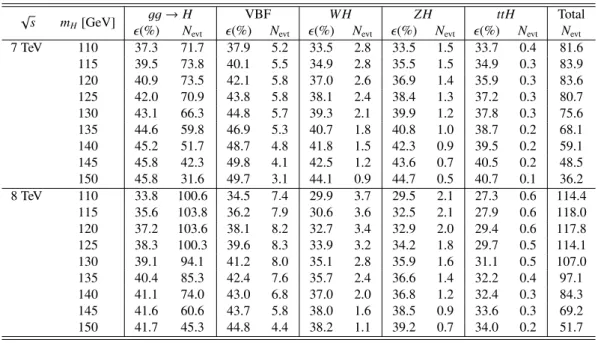
6.2 Signal e ffi ciency and yield
The expected Higgs boson signal efficiency and yields are computed and summarized in Table 5. The expected signal yield for the different production processes is normalized to an integrated luminosity of 4.8 fb
−1for the
√s
=7 TeV data and to 5.9 fb
−1for the
√s
=8 TeV data, along with the selection
Table 5: Expected Higgs boson signal efficiency
ǫ(including acceptance of kinematic selections as well as photon identification and isolation efficiencies) and event yield for H
→ γγassuming an integrated luminosity of 4.8 fb
−1for the
√s
=7 TeV data (top) and of 5.9 fb
−1for the
√s
=8 TeV data (bottom).
Results are given for different production processes.
√s mH[GeV] gg→H VBF W H ZH ttH Total
ǫ(%) Nevt ǫ(%) Nevt ǫ(%) Nevt ǫ(%) Nevt ǫ(%) Nevt Nevt
7 TeV 110 37.3 71.7 37.9 5.2 33.5 2.8 33.5 1.5 33.7 0.4 81.6
115 39.5 73.8 40.1 5.5 34.9 2.8 35.5 1.5 34.9 0.3 83.9
120 40.9 73.5 42.1 5.8 37.0 2.6 36.9 1.4 35.9 0.3 83.6
125 42.0 70.9 43.8 5.8 38.1 2.4 38.4 1.3 37.2 0.3 80.7
130 43.1 66.3 44.8 5.7 39.3 2.1 39.9 1.2 37.8 0.3 75.6
135 44.6 59.8 46.9 5.3 40.7 1.8 40.8 1.0 38.7 0.2 68.1
140 45.2 51.7 48.7 4.8 41.8 1.5 42.3 0.9 39.5 0.2 59.1
145 45.8 42.3 49.8 4.1 42.5 1.2 43.6 0.7 40.5 0.2 48.5
150 45.8 31.6 49.7 3.1 44.1 0.9 44.7 0.5 40.7 0.1 36.2
8 TeV 110 33.8 100.6 34.5 7.4 29.9 3.7 29.5 2.1 27.3 0.6 114.4
115 35.6 103.8 36.2 7.9 30.6 3.6 32.5 2.1 27.9 0.6 118.0
120 37.2 103.6 38.1 8.2 32.7 3.4 32.9 2.0 29.4 0.6 117.8
125 38.3 100.3 39.6 8.3 33.9 3.2 34.2 1.8 29.7 0.5 114.1
130 39.1 94.1 41.2 8.0 35.1 2.8 35.9 1.6 31.1 0.5 107.0
135 40.4 85.3 42.4 7.6 35.7 2.4 36.6 1.4 32.2 0.4 97.1
140 41.1 74.0 43.0 6.8 37.0 2.0 36.8 1.2 32.4 0.3 84.3
145 41.6 60.6 43.7 5.8 38.0 1.6 38.5 0.9 33.6 0.3 69.2
150 41.7 45.3 44.8 4.4 38.2 1.1 39.2 0.7 34.0 0.2 51.7
efficiencies. The last column displays the total expected number of H
→ γγsignal events after the application of the event selection specified above, depending on the Higgs boson mass. The composition of the different categories is given in Table 6.
6.2.1 Systematic uncertainty on the expected signal yields
In this section a brief description of the systematic uncertainties considered for the calculation of the expected signal yields with MC is given.
•
Luminosity. The uncertainty on the integrated luminosity is 1.8% for the
√s
=7 TeV data and 3.6% for the
√s
=8 TeV data [69].
•
Trigger Efficiency. The uncertainty on the trigger efficiency is 1% per event (see Sec.3.3).
•
Photon identification. The uncertainty on the photon identification is based on the comparison of the efficiency obtained using MC and various data-driven measurements based on photons from Z
→e
+e
−γ, electrons fromZ
→e
+e
−and a sideband technique. For the neural-network photon identification, a relative systematic uncertainty of 4% is assigned per photon for most
ηregions (for unconverted photons the uncertainty is 5% for 1.52
<|η|<1.81 and 7% in 1.81
<|η|<2.37).
Treating the uncertainty as fully correlated between the two photons, this translates to a relative uncertainty on the efficiency per event of 8.4%. For the tight identification used for the analysis of the
√s
=8 TeV data, a 5% relative uncertainty is assigned for photons in the barrel region of
the calorimeter,
|η|<1.37, and a 7% uncertainty is assigned for photons in the calorimeter endcap
region, 1.52
<|η|<2.37. Treating the uncertainties as fully correlated between the two photons,
this results in a relative event-level uncertainty of 10.8%.
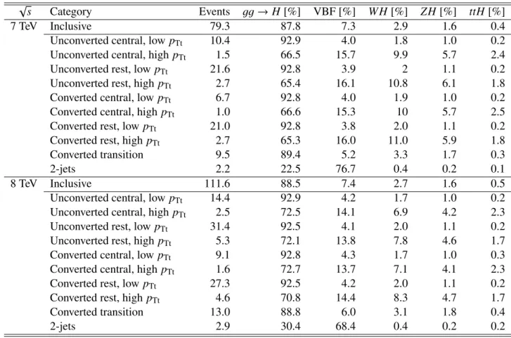
Table 6: Number of expected signal events per category at m
H =126.5 GeV, at
√s
=7 TeV (top) and
√
s
=8 TeV (bottom) and breakdown by production process.
√
s Category Events
gg→H [%] VBF [%] W H [%] ZH [%] ttH [%]
7 TeV Inclusive 79.3 87.8 7.3 2.9 1.6 0.4
Unconverted central, low p
Tt10.4 92.9 4.0 1.8 1.0 0.2
Unconverted central, high p
Tt1.5 66.5 15.7 9.9 5.7 2.4
Unconverted rest, low p
Tt21.6 92.8 3.9 2 1.1 0.2
Unconverted rest, high p
Tt2.7 65.4 16.1 10.8 6.1 1.8
Converted central, low p
Tt6.7 92.8 4.0 1.9 1.0 0.2
Converted central, high p
Tt1.0 66.6 15.3 10 5.7 2.5
Converted rest, low p
Tt21.0 92.8 3.8 2.0 1.1 0.2
Converted rest, high p
Tt2.7 65.3 16.0 11.0 5.9 1.8
Converted transition 9.5 89.4 5.2 3.3 1.7 0.3
2-jets 2.2 22.5 76.7 0.4 0.2 0.1
8 TeV Inclusive 111.6 88.5 7.4 2.7 1.6 0.5
Unconverted central, low p
Tt14.4 92.9 4.2 1.7 1.0 0.2
Unconverted central, high p
Tt2.5 72.5 14.1 6.9 4.2 2.3
Unconverted rest, low p
Tt31.4 92.5 4.1 2.0 1.1 0.2
Unconverted rest, high p
Tt5.3 72.1 13.8 7.8 4.6 1.7
Converted central, low p
Tt9.1 92.8 4.3 1.7 1.0 0.3
Converted central, high p
Tt1.6 72.7 13.7 7.1 4.1 2.3
Converted rest, low p
Tt27.3 92.5 4.2 2.0 1.1 0.2
Converted rest, high p
Tt4.6 70.8 14.4 8.3 4.7 1.7
Converted transition 13.0 88.8 6.0 3.1 1.8 0.4
2-jets 2.9 30.4 68.4 0.4 0.2 0.2
•
Isolation cut efficiency. The comparison of the isolation cut efficiency on Z
→e
+e
−between data and MC, where a relative shift between the mean of the isolation distribution between data and simulation of about 80 MeV is observed, gives an uncertainty of 0.4% (0.5%) per event for
√
s
=7(8) TeV.
•
Event pileup effect. The impact of event pileup on the expected yield is studied by comparing a sample with a mean number of proton-proton interactions of less than 10 (18) with a sample with a mean number of interactions of more than 10 (18) for the
√s
=7(8) TeV analysis, and is found to be 4%.
•
Photon energy scale. Evaluated as described in Sec. 6.3.2 for the mass shift, the uncertainty in the photon energy scale leads to a 0.3% uncertainty on the H
→γγyield.
•
Higgs boson production cross section. The theoretical uncertainties of the Higgs boson production
cross section for the different production processes are taken from [47, 67] (see Table 7). The
QCD perturbative uncertainties for the gluon fusion process are considered separately for the 2-
jets category and the remaining categories (see jet binning below). The uncertainties related to
the parton distribution functions are estimated following the prescription in [70] and by using the
PDF sets of CTEQ [71], MSTW [72] and NNPDF [73]. They are assumed to be 100% correlated
among processes with identical initial states.
•
Higgs boson decay branching fraction. The uncertainty on the Higgs boson decay branching frac- tion to two photons is 5% [74].
•
Migration of signal events between categories:
–
Higgs boson kinematics. The uncertainty in the population of the p
Ttcategories due to the modeling of the Higgs boson kinematics is estimated by varying scales and PDFs used by HqT2 [47]. This variation leads to an uncertainty on the population of the different categories:
1.1% in the low-p
Tcategories, 12.5% in the high-p
Tcategories, and 9% in the 2-jets category.
–
Event Pileup effects. The impact of pileup on the population of the converted and uncon- verted categories due to the behavior of the photon reconstruction is studied by comparing a sample with a mean number of interactions of less than 10 (18) with a sample with a mean number of interactions of more than 10 (18) for the
√s
=7(8) TeV analysis. The difference in population between the two samples is taken as an estimate of the uncertainty and it is found to be 3% (2%) for categories with unconverted photons, 2% (2%) for categories with converted photons, and 2% (12%) for the 2-jets category, respectively.
–
Material description. The probability for a photon to convert depends on the amount of material it traverses before reaching the calorimeter. The fraction of events in the different categories is compared between the nominal simulation and a simulation sample where ad- ditional material amounting to 5% to 20%, depending on the detector region, has been added upstream of the calorimeter. The assigned uncertainty in the signal yield from this source amounts to 4% for categories with unconverted and 3.5% for categories with converted pho- tons.
–
Primary vertex selection. The quantity
Pp
2T, evaluated for signal and background, used for the identification of the primary vertex, has been varied by an amount larger than the difference observed between data and MC. The effect on the expected yield in the different categories is smaller than 0.1% and is neglected.
–
Jet energy scale and resolution. The uncertainties on the jet energy scale is evaluated by varying the scale corrections within their respective uncertainties [27]. The uncertainty for the different classes of categories and different production processes amount to up to 19%
for the 2-jets category, and up to 4% for the other categories. The effect on the event yield of varying the jet resolution within its uncertainty is found to be negligible.
–
Jet binning. Following [75] the perturbative uncertainty on the gluon fusion contribution to the 2-jets category is evaluated separately and treated independently from the total cross section uncertainty. It is enhanced in this limited region of phase space due to the presence of higher-order logarithmic contributions. It is found to be 25% on the event yield from the gluon fusion process in the 2-jets category [76].
–
Underlying event. The uncertainty due to the modeling of the underlying event is estimated by comparing different underlying event tunes in the simulation [35]. The AUET2B tune is used for the default results, while the Perugia2011 tune is used for systematic studies. For the 2-jets category, a 30% uncertainty is assigned to the contribution from gluon fusion and the associated production processes, and a 6% uncertainty is assigned to the contribution from vector-boson fusion.
–
Jet-vertex-fraction. The systematic uncertainty on the choice of the jet-vertex-fraction re- quirement is estimated from the differences of efficiencies between data and MC simulation in Z
+2 jets events. For the
√s
=8 TeV analysis, a 13% uncertainty is assigned.
All systematic uncertainties, except for the uncertainty on the integrated luminosity, are treated as fully correlated between the
√s
=7 TeV and the
√s
=8 TeV analyses.
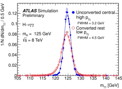
[GeV]
γ
mγ
105 110 115 120 125 130 135 140 145
/ 0.5 GeVγγ1/N dN/dm
0 0.02 0.04 0.06 0.08 0.1
0.12 ATLASSimulation
Preliminary Unconverted central high pTt
Converted rest low pTt
γ γ
→ H
= 125 GeV mH
= 8 TeV s
FWHM = 3.2 GeV
FWHM = 4.5 GeV
Figure 5: Invariant mass distributions for a Higgs boson with m
H =125 GeV, for the best-resolution cat- egory (Unconverted central, high p
Tt) shown in blue and for a category with lower resolution (Converted rest, low p
Tt) shown in red (see Table 2), for the
√s
=8 TeV simulation. The invariant mass distribution is parametrized by the sum of a Crystal Ball function and a broad Gaussian, where the latter accounts for fewer than 12% of events in all categories (fewer than 4% in most categories).
6.3 Diphoton mass modeling
The probability density function for the signal is modeled by the sum of a Crystal Ball function (CB) [77]
(taking into account the core resolution and a non-Gaussian tail towards lower mass values) and a small, wider Gaussian component (taking into account outliers in the distribution). The CB function is defined as
N
·
e
−t2/2if t
>−α(
|nα|)
n·e
−|α|2/2·(
|nα|− |α| −t)
−notherwise (1) where t
=(m
γγ−m
H−δmH)/σ
CB, N is a normalization parameter, m
His the hypothesized Higgs boson mass,
δmHis a category dependent offset,
σCBrepresents the diphoton invariant mass resolution, and n and
αparametrize the non-Gaussian tail. Table 2 shows the expected mass resolution for a Higgs boson with m
H =126.5 GeV for the different categories. Fig. 5 shows the resolution function for the categories with the best resolution and another with lower resolution. To extract the parameters from the signal simulation, a simultaneous fit to samples for different Higgs boson masses for each category is performed, exploiting the fact that the shape parameters are either linearly dependent on the Higgs boson mass, or to a good approximation independent of the Higgs boson mass.
6.3.1 Systematic uncertainty on the diphoton mass resolution
The following systematic uncertainties on the invariant mass resolution are considered:
•