Di ff erential cross sections of the Higgs boson measured in the diphoton decay channel with the ATLAS detector

ATLAS-CONF-2013-072 20/07/2013

ATLAS NOTE

ATLAS-CONF-2013-072

July 18, 2013

Minor revision: July 20, 2013

Di ff erential cross sections of the Higgs boson measured in the diphoton decay channel with the ATLAS detector

using 8 TeV proton-proton collision data

The ATLAS Collaboration

Abstract

This note presents differential cross section measurements of the Higgs boson, per- formed in the diphoton decay channel. The dataset used corresponds to 20.3 fb^-1of proton- proton collisions at √

s=8 TeV, produced by the LHC and collected by the ATLAS detector in 2012. With its high signal selection efficiency the diphoton decay channel is well suited to probe the underlying kinematic properties of the signal production and decay. Measure- ments for several diphoton and jet distributions are made for isolated photons within the geometric acceptance of the detector and they are corrected for experimental acceptance and resolution. Results are compared to theoretical predictions at the particle level.

Revised legend on Figure 9 in the Appendix with respect to the version on July 18, 2013

c

Copyright 2013 CERN for the benefit of the ATLAS Collaboration.

Reproduction of this article or parts of it is allowed as specified in the CC-BY-3.0 license.

1 Introduction

In 2012, the ATLAS and CMS collaborations observed a new particle [1, 2] in the search for the Stan- dard Model (SM) Higgs boson [3–5]. With additional data and an improved analysis strategy, ATLAS measured a combined total production rate of 1.33

0.21 times the SM Higgs boson expectation [6], and excluded a specific spin-2 hypothesis with a confidence level above 99.9% [7]. Spin and relative rates in the different production modes conform to the SM expectation, and in the diphoton channel ATLAS observed a signal with a local significance of 7.4

0.3 times the SM expectation [6].

Direct di

erential cross section measurements of the Higgs boson further elucidate its production and decay properties, and thus complement earlier analyses of its spin and couplings [6–8]. This note presents the measurement of eight Higgs boson observables in the diphoton decay channel. It is based on the full 2012 dataset recorded by the ATLAS detector, corresponding to 20.3 fb

of proton-proton collisions produced by the LHC at

s

8 TeV. The cross sections are measured within a fiducial region defined by two isolated photons within the geometrical acceptance of the detector. For each di

erential measurement, the dataset is divided in bins of the observable, and the resonant signal yield is separated from the dominant, continuum diphoton and photon-jet backgrounds using signal plus background fits to the diphoton invariant mass spectrum for each of these bins. These yields are corrected for detector acceptance as well as resolution in the measured observable to determine the fiducial di

erential cross sections.

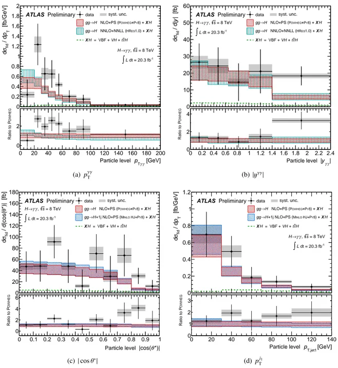
The eight observables studied are: the transverse momentum p

and rapidity

of the Higgs boson, the helicity angle

cos

in the Collins-Soper frame [9], the jet multiplicity N

in H

events and from that the jet veto fractions

for jet multiplicities i, the transverse momentum distribution of the leading jet p

, the azimuthal angle between the leading and the subleading jet

, and the transverse component of the vector sum of the momenta of the Higgs boson and dijet system

p

.

Directly measuring the transverse momentum, rapidity, and mass of the diphoton system determines the kinematic properties of the Higgs boson. Inclusive Higgs boson production is dominated by gluon- gluon fusion (ggH), for which the transverse momentum of the Higgs boson is largely balanced by the emission of soft gluons. Measuring p

thus directly probes the understanding of perturbative QCD calculations for this process. The rapidity distribution of the Higgs boson is sensitive to QCD radiative corrections and the parton distribution functions of the colliding protons. The helicity angle is defined as the angle between the beam axis and the photons in the Collins-Soper frame of the Higgs boson, and has been used to study the spin of the Higgs boson. The jet multiplicity is sensitive to the relative rates of the Higgs boson production mechanisms. Inclusive and 0-jet events are dominated by

processes, with vector boson fusion (VBF) and associated production with a weak vector boson (W H/ZH) becoming more important in 1- and 2-jet events. The small rate of Higgs bosons produced in association with a t¯ t pair (t¯ tH) becomes relevant for N

2. With the measured jet multiplicities, the jet veto fractions can be calculated, defined as the ratio of exclusive to inclusive cross sections

. The exclusive and inclusive jet cross sections are defined as the cross section of Higgs boson production with exactly i jets and i or more jets, respectively. These ratios are sensitive to the strong coupling

, the theoret- ical description of quark and gluon radiation, and the relative rates of the production modes. In

the transverse momentum of the leading jet corresponds to the hardest QCD radiation in Higgs boson production. The spectrum can be compared to higher order predictions.

The remaining observables are defined only for the subset of events which have at least two jets.

The azimuthal angle between the leading and sub-leading jets measures angular correlations between the

radiated objects. In the

and VBF production modes, it is sensitive to the spin and CP eigenvalue

of the Higgs boson [10]. The transverse momentum of the Higgs boson and dijet system is often used

to discriminate VBF against the much more abundant

production. In VBF production, the com- bined diphoton and dijet system tends to be well-balanced in p

, since extra radiation is considerably suppressed. This causes a smaller p

than in the

process, where such a suppression is absent. In VBF searches, the discriminating power of p

is limited by the large theoretical uncertainties on the

2 jets contamination. In this early measurement, no additional cuts were applied to suppress the

production mode.

The note is organized as follows. The ATLAS detector is briefly described in Section 2. Simulated data samples are presented in Section 3, and event and object selection are defined in Section 4. Section 5 describes parameterizations of the distributions of the diphoton invariant mass for signal and background events. Uncertainties on the signal yields, and on migrations between bins of the observables, are item- ized in Section 6. These are followed by a description of the extraction of the binned signal yields, and of their unfolding, in Sections 7 and 8. The differential cross sections are presented and compared to theoretical predictions in Section 9. Conclusions are drawn in Section 10.

2 The ATLAS detector

The ATLAS detector [11] is a multipurpose particle physics experiment with forward-backward sym- metric cylindrical geometry. The inner tracking detector (ID) consists of a silicon pixel detector and a silicon microstrip detector, both covering the pseudorapidity

region

2.5; and a straw-tube transition radiation tracker, covering the pseudorapidity region

2.0.

The ID is surrounded by a thin superconducting solenoid which provides a 2 T magnetic field, and by the high granularity liquid-argon (LAr) sampling electromagnetic calorimeter. The electromagnetic calorimeter is divided into a central barrel (|η|

1.475) and endcap regions on either end of the detector (1.375

3.2). In the region matched to the ID (|η|

2.5), it is radially segmented into three layers.

The first layer has a fine segmentation in

1.4 and 1.5

2.4, to facilitate the separation of es and

s and to improve the resolution of the shower position and direction measurements. The second layer collects most of the total reconstructed energy, and the third layer is used to correct for leakage beyond the calorimeter. In the region

1.8, the electromagnetic calorime- ter is preceded by a presampler detector to correct for upstream energy losses. An steel-scintillator tile calorimeter gives hadronic coverage in the central rapidity range (|η|

1.7), while two copper

LAr hadronic calorimeters provide coverage over 1.5

3.2. The forward regions (3.2

4.9) are instrumented with LAr calorimeters for both electromagnetic and hadronic measurements. The muon spectrometer that surrounds the calorimeters is not used in the present analysis. The combination of all these systems provides charged particle measurements together with e

cient and precise photon mea- surements in the pseudorapidity range

2.5. Jets and missing transverse energy are reconstructed using energy deposits over the full coverage of the calorimeters,

4.9.

3 Monte Carlo simulations

The acceptance inside the fiducial volume of the detector, and the detector response, are simulated using Monte Carlo (MC) techniques. Simulated processes play three distinct roles in this analysis. (i) They provide shape templates for describing the signal in the diphoton mass spectrum (Section 5.1). (ii) They are used in evaluating the appropriateness of analytic shapes for the background (Section 5.2), which

1ATLAS uses a right-handed coordinate system with its origin at the nominal interaction point (IP) in the centre of the detector, and the z-axis along the beam line. The x-axis points from the IP to the centre of the LHC ring, and the y-axis points upwards. Cylindrical coordinates (r, φ) are used in the transverse plane,φbeing the azimuthal angle around the beam line.

Observables labelled transverse are projected into thexyplane. The pseudorapidity is defined in terms of the polar angleθas η=−ln[tan(θ/2)].

2

are critical for the extraction of the signal yield (Section 7). (iii) The relationship between the particle level signal decays and the simulated detector response provides information necessary to unfold the measured yields to obtain differential cross sections, as discussed in Section 8. The samples used are described below.

3.1 Signal samples

The Higgs boson production cross sections are computed at next-to-next-to-leading order (NNLO) in QCD for the

process [12–17]. POWHEG [18–20] is tuned to match calculations with finite mass effects and soft-gluon resummations up to next-to-next-to-leading logarithmic order (NNLL) [21–23].

Next-to-leading order (NLO) electroweak (EW) corrections from Refs. [24,25] are applied. These results are compiled in Refs. [26–28] assuming factorization between QCD and EW corrections. The cross section for the VBF process has been calculated with full NLO QCD and EW corrections [29–31], and approximate NNLO QCD corrections are applied [32]. The W H and ZH processes have been calculated at NLO [33] and at NNLO [34], and NLO EW radiative corrections from Ref. [35] are applied. The full NLO QCD corrections for t¯ tH are used [36–39]. The Higgs boson cross sections, branching ratios [40–42] and their uncertainties are compiled in Refs [23, 43].

The Higgs boson production and decay are simulated separately for 11 values of the Higgs boson mass m

in 5 GeV steps from 100 to 150 GeV, in order to create a parameterization of the reconstructed signal line shape as a function of m

(Section 5.1). The five dominant production modes are simu- lated for each mass value. The normalization and factorization scales are set to the Higgs mass. The common ATLAS simulation tunes and parton distribution function (PDF) sets are used [44, 45]. Parton level

and VBF samples are generated using POWHEG with the CT10 PDF tune and interfaced to P

8 [46] to simulate the decay of the Higgs boson, showering and hadronization. Higgs bosons produced in association with a W or Z boson, or t¯ t, are generated with Pythia8 with the CTEQ6L1 PDF tune. The interaction of particles with the detector is simulated [47] using GEANT4 [48]. Effects from multiple interactions in a bunch crossing (pileup) are simulated by overlaying each signal event with a variable number of simulated inelastic proton-proton collisions, such that the distribution of this number of interactions agrees data.

The Higgs boson to diphoton decays simulated with P

8 contain H

decays with

f f ¯ . These

events pass the full selection at a very low rate, and can enter the signal region. Due to an artificial upper limit on the

mass in P

8, the simulated

) is lower than the branching fraction calculated in Ref. [49]. The rate of H

decays is therefore reweighted to match this prediction. An uncertainty of 100% is applied to this reweighting, due to the limited knowledge of this branching fraction. The efficiency for simulated H

events to pass the full event selection is 18 times lower than for H

Resonant H

production interferes destructively with the

continuum. This reduces the overall size of the expected contribution from

for m

126.5 GeV [50]. The interference varies with

cos

ect reaches its maximum of 11% for

cos

near 1 (see Table 6, in the Appendix). The calculation was made in the low p

limit, so it is most valid in that realm. Interference effects in the presence of additional radiation, i.e.

extra jets, are not considered. The simulated signal decays are weighted to account for this e

ect for the yield extraction and unfolding. The impact of this interference is thus not removed in the measurement.

In principle, theoretical predictions should include this small correction when comparing to the cross sections presented.

Simulated signal events are reweighted to match the longitudinal spread of the beam spot observed

in data. The reconstructed photon energies are modified to correct the photon energy resolution, based

on the comparison of Z

ee events in data and simulation. To improve the description of the shapes of

the photon showers in simulation, the variables that describe these shapes are corrected to improve the agreement of the simulated and observed distributions [51].

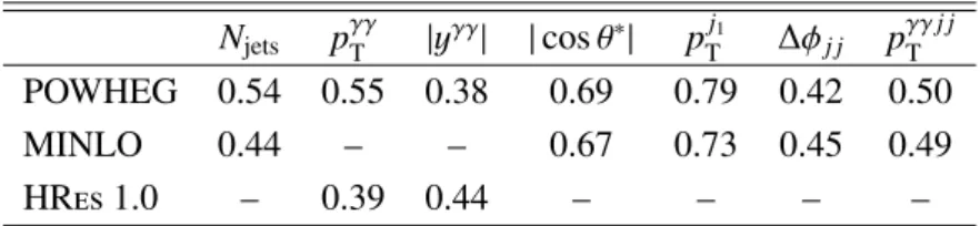
3.1.1 Higher-orderggHpredictions, for comparisons

For the later comparison with the unfolded cross sections, two higher-order predictions for

were produced. The multi-scale improved NLO, MINLO (rev. 2290) for H

1 jet [52] with the CT10 PDF set [44,45], and the NNLO+NNLL prediction of HRes (rev 1.0) [53], which uses the MSTW 2008 NNLO PDFs [54] and uses the infinite top quark mass approximation. Because HR

is a parton level prediction with an inclusive treatment of the QCD radiative correction, it is not possible to apply any isolation requirement on this sample (Section 4.2). MINLO was interfaced with Pythia8 for the simulation of underlying event, showering, and hadronization. Both samples were generated with m

126.8 GeV, the central value of the measured mass in the diphoton channel [6].

3.2 Background samples

Generated events are used to validate the analytical parameterization of the background shape in the diphoton invariant mass, and to estimate the systematic uncertainties from the parameterization itself.

The backgrounds from prompt diphoton and photon-jet processes (about 77% and 20% of the total back- ground) are simulated using S

[55], with up to three quark or gluon emissions from the matrix element using a leading order multijet merging algorithm. The jet-jet background, about 3% of the total background, is simulated with P

8. The Drell-Yan component, about 0.8% of the total background, does not significantly a

ect the shape of the background and is not considered. Due to the large number of simulated background events needed to validate the background shape in the diphoton invariant mass spectrum with negligible statistical uncertainty (Section 5), simulating the full detector acceptance and interaction is not feasible. The detector response to photons is parameterized as a smearing which de- pends on the transverse momentum and pseudorapidity. This procedure takes into account the varying resolutions and reconstruction efficiencies of different detector regions.

For each variable defined using jets, the particle level definition of the variable is smeared using a detector response matrix. This response matrix is derived from a sample of fully simulated diphoton plus jets events.

The method is validated by comparing the diphoton invariant mass shapes produced to that from fully simulated background events, and to the data events passing the event selection outside the signal region. A good agreement is observed within the statistical uncertainties.

4 Event selection

4.1 Event and photon selection in data

The event and object selection used in this analysis follows closely the approach of earlier ATLAS H

analyses, e.g. Ref. [56] where more details can be found. Events are recorded using a diphoton trigger with an e

ciency above 99% with respect to the o

ine selection, requiring two energy clusters that match criteria according to expectations for photon-induced electromagnetic showers. One of the clusters must have transverse energy, E

, greater than 35 GeV, and the other one must be greater than 25 GeV. They must lie within the fiducial acceptance of

2.37, excluding the transition region between the barrel and endcap calorimeters, 1.37

1.56. Basic data quality requirements ensure that all necessary components of the detector are operational.

The photon energies are calibrated based on a detailed simulation of the detector geometry and response. The calibration is refined by applying

in situ, from

4

studies of Z

ee decays. These factors range from

of the photon [57].

A primary vertex is selected for the event using a neural network combining the ‘pointing’ infor- mation of the photons in the calorimeters and the tracks of converted photons, with the

p

and

p

of tracks associated to a vertex, and the

between the diphoton system and the sum of the tracks’

momenta. The photon pointing determines the vertex position along the beam axis by combining infor- mation from the longitudinal segmentation of the calorimeter with a constraint from the average beam spot position. The z-position of the selected vertex is then used to correct the

and hence E

of the two photons.

Each photon of the pair must further satisfy isolation requirements from the inner detector and calorimeter. The total energy in a cone around the photon of

R

(

(

0.4 must be less than 6 GeV. A core region around the photon shower is excluded from that total energy and there are further corrections for the energy leakage from this core region into the outer cone. Energy from the underlying event or from minimum bias interactions (pileup) occurring in the same or neighboring bunch crossings is removed on an event-by-event basis [58]. The scalar sum of the p

of tracks originating from the diphoton vertex with p

1 GeV and in a cone of

R

0.2 must also be less than 2.6 GeV.

In order to simplify the shapes of the diphoton invariant mass distributions of backgrounds in the yield extractions, cuts are imposed not on the absolute E

s of the photons but on the ratios of each photon’s E

to their combined mass: E

0.35 (0.25) for the higher-E

(lower-E

) photon of the pair. Finally, the mass of the selected pair must satisfy 105 GeV

m

160 GeV. With 20.3 fb

of data in 2012, ATLAS collected 94135 events satisfying these requirements. Expected signal yields from MC are listed in Table 1.

4.2 Fiducial and particle level definitions

The particle level fiducial definition is chosen to mirror the event selection in data. This minimizes the extrapolation from detector level to particle level quantities. The selection criteria are as follows: the two highest-E

, isolated final state photons, within

2.37 and with 105 GeV

m

160 GeV are selected. Note that the transition region between the barrel and endcap calorimeters is not removed in this definition. After the pair is selected, the same cut on E

is applied as in the event selection in data: E

0.35 (0.25) for the two photons.

The isolation criterion is defined as follows: the sum of the p

of all stable particles

excluding muons and neutrinos is required to be less than 14 GeV within

R

0.4 of the photon. This requirement was found to correspond approximately to the calorimetric isolation cut of 6 GeV at reconstruction level.

The track isolation cut at detector level is much looser, and does not impact the derivation of this value.

This isolation requirement dramatically reduces the rate at which non-signal photons are selected. It also reduces the dependence of the measured cross sections on the model used to generate the unfolding corrections, by allowing for a more reliable relationship between photons produced in the fiducial region and those selected in the analysis (see Section 8).

4.3 Jet selection

Jets are selected both at particle and reconstruction level, using the anti-k

algorithm [59] with a distance parameter of R

0.4. At reconstruction level, the inputs are clusters of energy in the electromagnetic and hadronic calorimeters. At particle level all stable particles excluding muons and neutrinos serve as input.

The jet must have transverse momentum exceeding 30 GeV, and rapidity

4.4. Jets are calibrated using event-by-event corrections based on the energy density and simulated instrumental effects [58]. A

2A particle is considered stable if it has a lifetime of more than 10 ps.

Fiducial Fully Simulated and Selected Signal

Signal (MC) Yield

[%] VBF [%] W H [%] ZH [%] t¯ tH [%]

Inclusive 612 407 87.9 7.3 2.8 1.6 0.5

≥

1 Jet 252 180 76.3 15.1 4.8 2.7 1.1

≥

2 Jets 85 64 59.4 25.6 7.6 4.4 2.9

Table 1: Expected selected yields for the Standard Model at

s

8 TeV with m

125 GeV. The relative fractions selected in the five production modes,

W H, ZH, and t¯ tH are detailed. The fiducial signal is calculated at generator level.

residual correction from in situ measurements is applied to refine the jet calibration. Jets within

R

0.4 of either of the selected photons, or

R

0.2 of any electron, are vetoed. Electrons are not otherwise used in this analysis. Their selection criteria are identical to Ref. [6].

To reduce the pileup dependence at reconstruction level, jets with

2.4 and p

50 GeV must be consistent with originating from the selected primary vertex. This is ensured by considering the ratio of the (scalar) p

sum of tracks within the jet coming from the primary vertex, over the (scalar) p

sum over all tracks associated to that jet. This ‘jet vertex fraction’ (JVF) is required to exceed 0.25. If no tracks can be found to perform the test, the jet is kept.

5 Signal and background modelling

5.1 Signal modelling

The SM Higgs boson signal produces a narrow peak in m

, with a width completely dominated by the detector resolution. This shape is modelled analytically using a Crystal Ball function [60] plus a wide Gaussian component for modelling tails in the resolution function. Most parameters of this model are constant with respect to the hypothesized Higgs boson mass m

, while the width increases with m

and is well-described as a linear function of it. A simultaneous fit to signal MC samples at di

erent masses is performed to determine the constant parameters and the evolution of the width. This provides a parameterized signal shape for values of m

where MC samples are not available. This procedure is performed separately for each bin in each observable that is considered. The fitted width at the central value of the measured Higgs boson mass m

126.8 GeV is provided in the Appendix for each variable and bin.

5.2 Background modelling

The analytical function used to describe the background in the diphoton mass spectrum is selected in each bin individually using the procedure below, which is intended to minimize potential bias.

The background samples described in Section 3.2 provide a reference shape with minimal statistical fluctuations. Using these shapes, potential background models are tested by performing signal plus background fits on this background-only sample. This test is made in 1 GeV steps, shifting the signal model in a window of 119

135 GeV, corresponding to a 16 GeV range centered around the Higgs boson mass. At each step, the measured (spurious) signal must be less than 20% of the statistical uncertainty on the background in the data or less than 10% of the yield of the expected SM signal. Two classes of models are evaluated: Bernstein polynomials and exponentials of polynomials of the form e

. The model with the lowest number of degrees of freedom that satisfies the requirements described above is selected. The largest bias found in the modeling of the MC background shape is taken as an uncertainty

6

on the observed signal yield for each observable. The resulting systematic is typically much smaller than the upper limits imposed here. The models and the assessed uncertainties are presented in the variables’

summary tables in the Appendix. The background shape in all bins is described using exponentials of polynomials of first and second order.

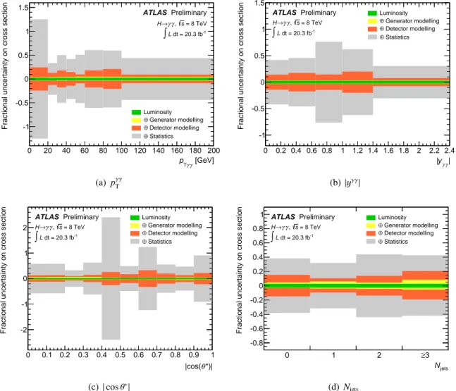
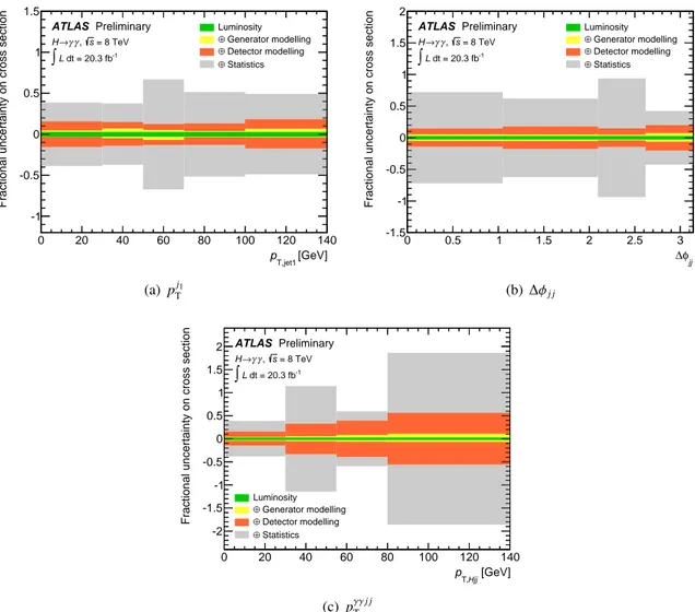
6 Experimental uncertainties

The measured di

erential cross sections are subject to uncertainties on the overall yield and on migrations between bins of the observables. Further, the signal resolution affects the fitted shape, so resolution uncertainties have an important impact on the measured yield. Uncertainties on the energy scale and signal peak position do not appreciably impact the measured yields. The uncertainties described here are evaluated according to the methods used in Ref. [56].

6.1 Uncertainties on the yield

Uncertainties on the luminosity, trigger, and identification and isolation e

ciencies impact the expected number of events. A bias from a poor choice of background function would change the extracted yield.

•

The uncertainty on the integrated luminosity is obtained from beam separation scans taken in April 2012. It is found to be 2.8%, following the method presented in Ref [61].

•

The uncertainty on the trigger efficiency is measured using a ‘boot-strapping’ method from mini- mum bias events as described in Ref. [62], and found to be 0.5%.

•

The single-photon identification efficiency and its uncertainties are evaluated in data. These un- certainties are propagated into the diphoton topologies, according to the method described in Ref. [56]. The event level uncertainty of 2.4% is found to be constant across bins of the di

erential variables.

•

The e

ciencies of the combined calorimetric and tracking isolation cuts are measured with Z

ee MC and data, and the difference is assigned as an uncertainty. For the non-jet inclusive variables and p

this amounts to a 1% uncertainty. A 2% uncertainty applies to the two-jet variables. For the N

spectrum, the uncertainty increases by bin: 1% for the first two bins, 2% for the 3rd, and 4% for the final bin.

•

The uncertainty on the signal yield from the background shape is described in Section 5.2 and presented in the Appendix.

6.2 Uncertainties on photon energy resolution

The calorimeter energy resolution is measured in data using electrons from Z decays. Its uncertainty, together with the uncertainty on the extrapolation from electrons to photons, accounts for a 22-31%

uncertainty on the resolution of the signal in the diphoton invariant mass, depending on the observable and bin. The resolution uncertainties are included in the fit and are transformed into yield uncertainties, as described in Section 7.2.

6.3 Migration uncertainties

Three sources of uncertainties are considered for the variables that are based on jets: jet energy resolution

(JER) and scale (JES), jet vertex fraction (JVF), and jets from pileup (that do not originate from the

primary vertex).

The jet energy scale and resolution uncertainties are estimated by applying shifts and smearings to the jet energy within their expected uncertainties. These shifts are derived in situ, exploiting the transverse momentum balance in

Z

jet energy scale for these measurements lead to a set of baseline uncertainties. The most important JES uncertainties for this analysis are from the

forward jets, and due to the unknown composition and modelling of the associated calorimeter response of quark and gluon initiated jets.

Uncertainties from JVF modelling are quantified by varying the JVF cut up and down according to its uncertainty around the nominal cut value of 0.25. The JVF uncertainty is estimated by comparing simulation with data in Z

jet events and is parametrized as a function of jet p

and

The uncertainty associated with the modelling of jets originating from pileup interactions is evaluated by randomly subtracting a fraction of the simulated pileup jets. The fraction of pileup jets removed is estimated by comparing the data to MC ratio of jets in pile-up enriched control regions of Z

jets events.

The combined impact of these uncertainties on the signal yields ranges from 3-15% according to the observable and bin, and is tabulated in the Appendix.

Migration effects due to the photon energy scale, between bins in the cross section observables, were estimated to be negligible.

The contamination of the jet related observables, due to the occurrence of double parton interaction (DPI) in the context of simultaneous dijet and Higgs boson production, were found to be negligible.

The e

ect was evaluated using the expected dijet cross section for the jet requirements presented in Section 4.3, with the measured e

ective area parameter for hard DPI [63].

7 Signal extraction

7.1 Binning of the observables

The dataset is divided into bins of the observables and the signal yield in each bin is extracted using an extended unbinned likelihood fit to the diphoton invariant mass distribution. The binning was chosen to allow differential measurements, with statistics sufficient for a significant measurement in each bin, using the expected signal yields from simulation. The nominal target significances were 2

(1.5

bin for the inclusive (2-jet) variables. To obtain a reliable unfolding, the migrations between bins in the reconstructed distributions must be small. The binnings chosen based on these considerations are displayed in the variable summary tables in the Appendix.

7.2 Fit procedure and likelihood

An unbinned fit of the diphoton invariant mass is performed simultaneously in all bins, for each ob- servable. The Higgs boson mass m

and the nuisance parameters on the signal shape and position are common among all bins for each observable. The likelihood function maximized has the form

L(m_γγ

;

m

)

i











e

n

!

n_i

Y

j

hν^sig_i S_i

(m

; m

)

(m

)











× Y

k

G_k

(1)

with

and

being the number of signal and background events estimated in data in the i

bin of the observable,

the mean value of the underlying Poisson distribution of the n

events, and m

is the diphoton mass for event j. The signal probability density functions (PDF)

described in Section 5.1 depend on the Higgs boson mass m

and on nuisance parameters from the energy resolution and scale.

8

The background PDFs

are chosen as described in Section 5.2. The term

is a function of the k

nuisance parameters and implements constraints from the photon energy resolution and scale into the fit. Uncertainties that do not affect the shape of the fit, for instance the background model uncertainty or trigger yield, are not included at this stage. Rather, they are applied during the unfolding procedure (Section 8).

For observables where a set of events is not included in the measured spectrum, the un-categorized events are placed into an additional bin, which is included in the fit. These include, for example, events with p

larger than the upper edge of the highest bin, or events with 0 or 1 jet for

. The events in this additional bin help to constrain the Higgs boson mass and other nuisance parameters.

The fitted yields and errors are validated using an ensemble of pseudo-experiments and the statistical component of the error on the total yield is separated using a second fit with the nuisance parameters fixed to their profiled values.

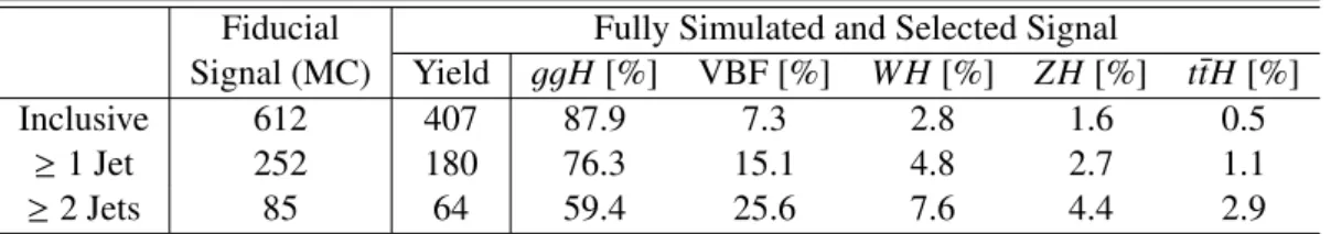
Results for the diphoton invariant mass fit are shown for the jet multiplicity binning, as an example, in Figure 1. The determined yields for the inclusive and dijet observables are shown in Figures 2 and 3. The yields of all observables are in good agreement with the simulated SM expectation at m

125 GeV.

8 Unfolding procedure and associated uncertainties

8.1 Procedure

The data yields extracted in the previous section are corrected for detector e

ects using bin-by-bin fac- tors. These are derived as the ratio of the yields from particle level to reconstruction level from simulated Higgs boson events, according to the SM expectation listed in Table 1. In each bin,

c

n

i /nReconstructed

i

(2)

is used to correct the extracted signal yield in data. This unfolding procedure corrects for all efficien- cies, acceptances, and resolution effects. The correction factors range from 1.2 to 1.8, and include the extrapolation (about 20%, across all bins and observables) over the small region in

excluded from reconstructed photon candidates (Section 4.1).

The method is formally unbiased provided that c

c

. In practice, the requirement to use this method is that the ‘purity’ of events reconstructed into the same bin in which they were generated should not be too low. Among the measured observables, p

,

cos

have very high purity (> 87%);

for the jet variables, it can be as low as 50%. The lower purity for the jet variables may be understood as a ‘double migration’: first for passing or failing the jet definition, and second for the migrations of the observable. The purities and derived correction factors for each bin of each observable are presented in the summary tables in the Appendix.

8.2 Uncertainties on the correction factors

To the extent that the physics processes and simulation model do not perfectly reproduce the data, the correction factors defined in Eq. 2 will be biased and model dependent. This dependence must be fully evaluated and considered as an uncertainty on the method. The potential bias can be categorized in two aspects: sample composition and shape.

The sample composition and description a

ect correction factors, because di

erent production pro-

cesses or generators may have different reconstruction level efficiencies. For instance the larger jet activ-

ity in t¯ tH events results in lower isolation efficiencies and larger correction factors than

of the input distributions matter, because the net migrations in a distribution will be from a more popu-

lated bin towards its less populated neighbour. The uncertainties from these considerations are evaluated

by manipulating the Monte Carlo from which the correction factors are determined, in four ways:

[GeV]

γ mγ

110 120 130 140 150 160

Events / GeV

500 1000 1500 2000 2500

Data Sig+Bkg Fit Bkg

Preliminary ATLAS

= 8 TeV s γ, γ

→

→H pp

dt = 20.3 fb-1

∫L

jets = 0 N

[GeV]

γ

mγ

110 120 130 140 150 160

Data-Bkg

-100 0 100 200

(a) Njets=0

[GeV]

γ mγ

110 120 130 140 150 160

Events / GeV

100 200 300 400 500 600 700 800 900

Data Sig+Bkg Fit Bkg

Preliminary ATLAS

= 8 TeV s γ, γ

→

→H pp

dt = 20.3 fb-1

∫L

jets = 1 N

[GeV]

γ

mγ

110 120 130 140 150 160

Data-Bkg

-50 0 50 100

(b)Njets=1

[GeV]

γ mγ

110 120 130 140 150 160

Events / GeV

50 100 150 200 250 300

Data Sig+Bkg Fit Bkg

Preliminary ATLAS

= 8 TeV s γ,

→γ

→H pp

dt = 20.3 fb-1

∫L

jets = 2 N

[GeV]

γ

mγ

110 120 130 140 150 160

Data-Bkg

-50 0 50

(c) Njets=2

[GeV]

γ mγ

110 120 130 140 150 160

Events / GeV

20 40 60 80 100 120

Data Sig+Bkg Fit Bkg

Preliminary ATLAS

= 8 TeV s γ,

→γ

→H pp

dt = 20.3 fb-1

∫L

≥ 3 Njets

[GeV]

γ

mγ

110 120 130 140 150 160

Data-Bkg -20

0 20

(d)Njets≥3

Figure 1: Diphoton invariant mass distributions are presented for the 4 bins of the N

extraction.

The curves show the results of the single simultaneous fit to data for all N

bins. The red line is the combined signal and background PDF, and the dashed line shows the background PDF. The difference of the two curves is the extracted signal yield. The bottom inset displays the residuals of the data with respect to the fitted background component, and the dotted red line corresponds to the signal PDF.

10

[GeV]

γ γ

pT

Reconstructed ]-1 [GeV Tp / dNd

0 5 10 15 20

25 ATLAS Preliminary

= 8 TeV s γ, γ

→ H

∫L dt = 20.3 fb^-1 data syst. unc.

H X ) + 8 PY

+ OWHEG NLO+PS (P

→H gg

H t t + VH = VBF + H X

[GeV]

γ γ

pT

Reconstructed

0 20 40 60 80 100 120 140 160 180 200

OWHEGRatio to P

0 2

(a) p^γγ_T

γ| yγ

| Reconstructed

|y / d|Nd

0 100 200 300 400 500 600 700 800

Preliminary ATLAS

= 8 TeV s γ, γ

→ H

∫L dt = 20.3 fb^-1

data syst. unc.

H X ) + 8 PY

+ OWHEG NLO+PS (P

→H gg

H t t + VH = VBF + H X

γ| yγ

| Reconstructed 0 0.2 0.4 0.6 0.8 1 1.2 1.4 1.6 1.8 2 2.2 2.4

OWHEGRatio to P

0 2 4

(b)|y^γγ|

θ*)|

|cos(

Reconstructed

*)|θ / d|cos(Nd

0 200 400 600 800 1000 1200 1400 1600 1800 2000 2200 2400

Preliminary ATLAS

= 8 TeV s γ, γ

→ H

∫L dt = 20.3 fb^-1

data syst. unc.

H X ) + 8 PY

+ OWHEG NLO+PS (P

→H gg

H t t + VH = VBF + H X

θ*)|

|cos(

Reconstructed 0 0.1 0.2 0.3 0.4 0.5 0.6 0.7 0.8 0.9 1

OWHEGRatio to P

0 2 4 6

(c) |cosθ^∗|

[GeV]

T,jet1

p Reconstructed ]-1 [GeV Tp / dNd

0 2 4 6 8 10 12 14 16

Preliminary ATLAS

= 8 TeV s γ, γ

→ H

∫L dt = 20.3 fb^-1 data syst. unc.

H X ) + 8 PY

+ OWHEG NLO+PS (P

→H gg

H t t + VH = VBF + H X

[GeV]

T,jet1

p Reconstructed

0 20 40 60 80 100 120 140

OWHEGRatio to P

0 1 2 3

(d) p_T^j1

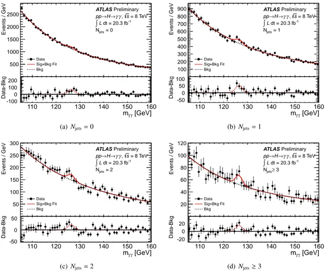
Figure 2: The fitted yield per bin for the Higgs p

, rapidity,

cos

p

are shown.

The bin below 30 GeV in the leading jet p

spectrum is populated by events with a jet multiplicity of

zero. The grey bands for each data point show the systematic uncertainty on the yields, while the black

bars represent the total systematic and statistical error. The hatched histogram shows the SM expectation

with m

125 GeV simulated with the full detector response and e

ciencies. Its spread corresponds to

the quadratic sum of the migration uncertainties outlined in Section 6, and theoretical uncertainties. The

theory uncertainties are due to missing higher order corrections, the PDF set adopted, the simulation of

the underlying event, and the H

branching fraction. The green line shows the contribution from

VBF, W H, ZH, and t¯ tH production.

Njets

Reconstructed

eventsN

0 50 100 150 200 250 300 350 400

450 ATLAS Preliminary

= 8 TeV s γ, γ

→ H

∫L dt = 20.3 fb^-1 data syst. unc.

H X ) + 8 PY

+ OWHEG NLO+PS (P

→H gg

H t t + VH = VBF + H X

Njets

Reconstructed

0 1 2 ≥3

OWHEGRatio to P

0 1 2 3

(a)Njets

φjj

∆ Reconstructed

φ∆ / dNd

0 20 40 60 80 100 120 140 160

180 ATLAS Preliminary

= 8 TeV s γ,

→γ H

∫L dt = 20.3 fb^-1 data syst. unc.

H X ) + 8 PY

+ OWHEG NLO+PS (P

→H gg

H t t + VH = VBF + H X

φjj

∆ Reconstructed

0 0.5 1 1.5 2 2.5 3

OWHEGRatio to P

0 5

(b)∆φj j

[GeV]

Hjj

pT,

Reconstructed ]-1 [GeV Tp / dNd

0 1 2 3 4

5 ATLAS Preliminary

= 8 TeV s γ, γ

→ H

∫L dt = 20.3 fb^-1 data syst. unc.

H X ) + 8 PY

+ OWHEG NLO+PS (P

→H gg

H t t + VH = VBF + H X

[GeV]

Hjj

pT,

Reconstructed

0 20 40 60 80 100 120 140

OWHEGRatio to P

0 2 4 6

(c) p^{γγj j}_T

Figure 3: The fitted yields for the jet multiplicity, the azimuthal angle between the leading and sublead- ing jet, and the p

of the summed Higgs and dijet are shown. See caption of Figure 2 for more details.

12

1. Alter the composition from the SM expectation by varying the relative VBF and W H

ZH fractions up (2×) and down (0.5×), motivated by the 1

contour presented in the H

coupling results [6]. Since the t¯ tH fraction is not well-constrained by those results, it is varied by factors of 6 and 0, motivated by the combined up variations necessary to fully cover the observed excess for large N

in data (Figure 5(a)).

2. Estimate the uncertainties from missing higher order perturbative corrections in

production, by varying the factorization and renormalization scales up (2×) and down (0.5×). To further test the dependence of the modelling of

production, replace the nominal POWHEG+Pythia8 sample with the leading order matrix element multijet merged prediction of S

.

3. Disable multi-parton interactions to test the dependence on the modelling of the underlying event.

4. Reweight the combined SM prediction in p

and

or p

spectra to match the unfolded results in these variables.

For each of these variations new correction factors are derived, and the shifts with respect to the nominal SM correction factor are assigned as uncertainties. These four methods are not orthogonal:

changing samples and reweighting impacts the predicted spectra. The full uncertainty is taken thus as the envelope of the data-based reweighting, with the quadratic sum of the composition, scale and underlying event variations.

9 Results and comparison to theoretical predictions

The unfolded differential cross sections and the jet veto fraction are displayed in Figures 4 and 5, for the fiducial region defined in Section 4.2. The fractional uncertainties of all observables are displayed in Figures 6 and 7. The break-down of all uncertainty sources and correlations are also tabulated in the Appendix. The

cos

distribution presented in Fig. 4(c) is compatible with the results of earlier, dedicated spin studies [64], where the signal yields were extracted under the assumption of a particular spin hypothesis and not unfolded.

The results are compared to MC predictions of the SM expectation. All predictions were generated at m

126.8 GeV, the central value of the measured Higgs boson mass in the diphoton channel [6].

This value of m

was used instead of the value from the combined measurement [6], in order to reduce uncertainties from the photon energy scale in the comparisons. For

three different predictions are considered (see Section 3.1): Higgs boson production at NLO POWHEG, Higgs boson

1 jet from MINLO at NLO, and HR

at NNLO

NNLL. The POWHEG prediction is shown for all 8 observables.

HRes is presented for p

and

associated Higgs boson production were simulated as outlined in Section 3.1.

All cross sections were scaled to the latest values from Ref. [43]. The band shown on the prediction is the linear sum of the uncertainties due to missing higher-order perturbative corrections and PDF

variations, added in quadrature with the uncertainty due to the underlying event modelling, the SM H

branching fraction, and the simulation statistics of the prediction in question. The PDF variations

were obtained using the 68% confidence interval eigentunes of the PDF sets. The uncertainties due to

the underlying event modelling are obtained by disabling multi-parton interactions; this uncertainty is

omitted for HR

. The uncertainties due to missing higher-order perturbative corrections were estimated

for each generator by correlated and uncorrelated variations of the renormalization and factorization

scales by factors of 2 and 0.5. The envelope of the largest deviations from the cross section at the

nominal scale m

is taken as the uncertainty. In the case of HR

the envelope of variations of the

resummation, renormalization, and factorization scales was used.

N

p

cos

p

p

POWHEG 0.54 0.55 0.38 0.69 0.79 0.42 0.50

MINLO 0.44 – – 0.67 0.73 0.45 0.49

HRes 1.0 – 0.39 0.44 – – – –

Table 2: Displayed are the probabilities from

tests for the agreement between the unfolded observa- tion and the theoretical predictions, calculated with the full covariance between bins of the observables.

The observed cross section in the fiducial region is higher than the SM expectation, in agreement with earlier analyses in the diphoton channel from ATLAS [6]. Within the limited statistics of the mea- surement, the predicted shapes agree well with the observation. Table 2 quantifies the agreement for all displayed predictions, by calculating the probabilities of

tests for all unfolded observables with respect to the predictions, taking into account the full covariance between the bins. The probabilities range from 0.38 (|y

with POWHEG) to 0.79 (p

with POWHEG). The HR

1.0 prediction of p

, for which the p-value is 0.39, will soon be superseded by Ref. [65], taking into account the finite quark mass e

ects.

The POWHEG prediction for

is not expected to perform well, because the emission of the second jet is made purely by the parton shower algorithm, and does not include any angular correlations from the matrix element. The theoretical uncertainties for large N

are unnaturally small, because scale vari- ations do not significantly shift the predictions from the parton shower algorithm. A more-conservative presentation of the theoretical uncertainties of this distribution is presented in Figure 8 in the Appendix.

Two additional NNLO

NNLL predictions from Refs. [66, 67] for p

are included as well, in Fig- ure 9.

10 Conclusions

This note presents direct measurements of differential cross sections of the Higgs boson in the diphoton channel, from 20.3 fb

of data at

s

8 TeV collected by the ATLAS experiment at the LHC in 2012.

These measurements are performed for the fiducial range of

2.37 and E

0.35 (0.25) for the leading (subleading) photon, and with 105 GeV

m

160 GeV. The variables presented describe the fundamental kinematic properties of the Higgs boson, probe its spin and parity, and test the theoretical description of QCD in its production. The di

erential cross-sections in seven observables are extracted by fits to the diphoton invariant mass spectrum: p

,

,

cos

, N

, p

,

, and p

. The jet veto fraction

is calculated from the N

distribution. The measured differential cross sections are compared with various theoretical predictions. Within the experimental and theoretical uncertainties, no significant deviation from the SM expectation is observed.

14