Measurements of the Higgs boson inclusive, differential and production cross sections in the 4`

A TLAS-CONF-2019-025 24/10/2019

ATLAS CONF Note

ATLAS-CONF-2019-025

15 July 2019

Measurements of the Higgs boson inclusive, differential and production cross sections in the 4`

decay channel at √

s = 13 TeV with the ATLAS detector

The ATLAS Collaboration

Inclusive, differential and production mode cross sections of the Higgs boson are meas- ured in the H → Z Z

→ 4 ` decay channel. Additionally, cross sections are measured for the main production modes in several exclusive regions of the Higgs boson produc- tion phase space. The used dataset corresponds to proton − proton collision data produced at the Large Hadron Collider at a centre-of-mass energy of 13 TeV and recorded by the ATLAS detector from 2015 to 2018, equivalent to an integrated luminosity of 139 fb

. The inclusive fiducial cross section for the process H → Z Z

→ 4 ` is measured to be σ

= 3 . 35 ± 0 . 32 fb, while the Standard Model prediction is σ

= 3 . 41 ± 0 . 18 fb. The cross-section times H → Z Z

branching ratio with the Higgs rapidity | y

| < 2.5 for gluon fusion and vector-boson fusion production are measured to be 1 . 15 ± 0 . 13 pb and 0 . 13 ± 0 . 04 pb, respectively. All measurements are in agreement with the Standard Model prediction.

Update 15 October 2019: Section 3 was updated to include additional references, and correct the pileup simulation software versions.

© 2019 CERN for the benefit of the ATLAS Collaboration.

Reproduction of this article or parts of it is allowed as specified in the CC-BY-4.0 license.

1 Introduction

The observation of the Higgs boson by the ATLAS and CMS experiments [1, 2] with the Large Hadron Collider (LHC) Run 1 data at centre-of-mass energies of

√

s = 7 TeV and 8 TeV has been a major step towards the understanding of the electroweak (EW) symmetry breaking mechanism [3–5].

Studies on the spin, parity, couplings, fiducial and differential cross sections of the new particle have been performed [6–28] showing no significant deviation from the Standard Model (SM) predictions for the Higgs boson with a mass of 125 GeV.

Updated measurements of the Higgs boson properties in the H → Z Z

→ 4 ` decay channel (where

` = e or µ ) are presented using 139 ± 2 fb

of proton-proton ( pp ) collision data collected at

√ s = 13 TeV at the LHC by the ATLAS detector between 2015 and 2018. Four types of measurements are reported:

inclusive and differential production cross sections in the fiducial phase space, cross sections within the Higgs boson rapidity of | y

| = 2 . 5 of production modes both inclusively and in several exclusive regions of the Higgs boson phase space. All measurements are performed under the assumption that the Higgs boson mass is 125 GeV, and are compared to Standard Model (SM) predictions.

The main differences with respect to the previous results [11, 12, 29] are: (i) full LHC Run 2 integrated luminosity, (ii) improved lepton isolation to mitigate the impact of additional pp interactions in the same bunch crossing (pileup), (iii) constraint of the major non-resonant Z Z

background from dedicated data sidebands, (iv) unfolding method for differential variables exploiting the detector response matrix, (v) additional reconstructed event categories in the analysis and new discriminants to enhance the sensitivity to the various production modes of the SM Higgs boson, (vi) dedicated control region to constraint the background in the analysis categories probing the ttH production.

The note is organised as follows: a brief introduction of the ATLAS detector is given in Section 2.

In Section 3, the data and simulated signal and background samples are described. The selection and categorisation of the Higgs boson candidate events is detailed in Section 4, while the background modelling is described in Section 5. The analysis strategy is outlined in Section 6. The experimental and theoretical systematic uncertainties, detailed in Section 7, are taken into account for the statistical interpretation of the data. The final results are presented in Section 8. Concluding remarks are given in Section 9.

2 The ATLAS detector

The ATLAS experiment [30] at the LHC is a multi-purpose particle detector with a forward-backward symmetric cylindrical geometry1 and a near 4 π coverage in solid angle. It consists of an inner tracking detector (ID) surrounded by a thin superconducting solenoid, which provides a 2 T axial magnetic field, electromagnetic (EM) and hadron calorimeters, and a muon spectrometer (MS). The inner tracking detector covers the pseudorapidity range |η| < 2 . 5. It consists of silicon pixel, including the newly installed insertable B-layer [31], silicon micro-strip, and transition radiation tracking detectors. Lead/liquid-argon (LAr) sampling calorimeters provide electromagnetic energy measurements with high granularity. A

1 ATLAS uses a right-handed coordinate system with its origin at the nominal interaction point (IP) in the centre of the detector and the z -axis along the beam pipe. The x -axis points from the IP to the centre of the LHC ring, and the y -axis points upwards.

Cylindrical coordinates (r, φ) are used in the transverse plane, φ being the azimuthal angle around the z -axis. The pseudorapidity is defined in terms of the polar angle θ as η = − ln tan ( θ / 2 ) . Angular distance is measured in units of ∆R ≡ p

(∆η )

+ (∆φ )

.

hadron (steel/scintillator-tile) calorimeter covers the central pseudorapidity range ( |η| < 1 . 7). The end-cap and forward regions are instrumented up to |η| = 4 . 9 with LAr calorimeters for both EM and hadronic energy measurements. The calorimeters are surrounded by the muon spectrometer and three large air-core toroidal superconducting magnets with eight coils each. The field integral of the toroid magnets ranges between 2.0 and 6.0 T m across most of the detector. The muon spectrometer includes a system of precision tracking chambers and fast detectors for triggering with a coverage of |η | < 2 . 7. Events are selected using a first-level trigger implemented in custom electronics, which reduces the event rate to a maximum of 100 kHz using a subset of detector information. Software algorithms with access to the full detector information are then used in the high-level trigger to yield a recorded event rate of about 1 kHz [32].

3 Signal and background simulation

The production of the SM Higgs boson via gluon-gluon fusion (ggF), via vector boson fusion (VBF), with an associated vector boson ( VH , where V is a W or a Z boson) and with a top quark pair ( ttH ) is modelled with the POWHEG-BOX v2 Monte Carlo (MC) event generator [33–40]. For ggF, the PDF4LHC next-to-next-to-leading-order (NNLO) set of parton distribution functions (PDF) is used, while for all other production modes, the PDF4LHC next-to-leading-order (NLO) set is used [41]. The ggF Higgs boson production uses the POWHEG method for merging the NLO Higgs + jet cross section with the parton shower and the MiNLO method [42] to simultaneously achieve NLO accuracy for inclusive Higgs boson production. In a second step, a reweighting procedure (NNLOPS) [43], exploiting the Higgs boson rapidity distribution, is applied using the HNNLO program [44, 45] to achieve NNLO accuracy in the strong coupling constant α

.

The matrix elements of the VBF, q q ¯ → VH and ttH production mechanisms are calculated up to NLO in QCD. For VH production, the MiNLO method is used to merge 0- and 1-jet events [40, 42]. The gg → Z H contribution is modelled at leading order (LO) in QCD.

The production of a Higgs boson in association with a bottom quark pair ( bbH ) is simulated at NLO with MadGraph5_aMC@NLO v2.3.3 [46], using the CT10 NLO PDF [47], while the production in association with a single top quark ( tH + X where X is either j b or W , defined in the following as tH ) are simulated at NLO with MadGraph5_aMC@NLO v2.6.0 using the NNPDF30 PDF set [48].

For all production mechanisms, with the exception of ttH 2, the PYTHIA 8 [50] generator, using the AZNLO set of tuned parameter [51], is used for the H → Z Z

→ 4 ` decay as well as for the parton shower modelling. The event generator is interfaced to EvtGen v1.2.0 [52] for simulation of the bottom and charm hadron decays. All signal samples are simulated for a Higgs boson mass m

= 125 GeV.

For additional cross checks, the ggF sample was also generated with MadGraph5_aMC@NLO. This simulation is accurate at NLO QCD accuracy for zero, one and two additional partons merged with the FxFx merging scheme [53, 54].

The Higgs boson production cross sections and decay branching ratios, as well as their uncertainties, are taken from Refs. [48, 55–62]. The ggF production is calculated with next-to-next-to-next-to-leading order (N

LO) accuracy in QCD and has NLO electroweak (EW) corrections applied [63–69]. For VBF production, full NLO QCD and EW calculations are used with approximate NNLO QCD corrections [70, 71]. The qq - and qg -initiated VH production is calculated at NNLO in QCD and NLO EW corrections

2 The A14 tune [49] is used for ttH sample.

are applied [72–74], while gg -initiated VH production is calculated at NLO in QCD. The ttH [75–78], bbH [79–81] and tH [82] processes are calculated to NLO accuracy in QCD. The branching ratio for the H → Z Z

→ 4 ` decay with m

= 125 GeV is predicted to be 0.0124% [59, 83] in the SM using PROPHECY4F [84, 85], which includes the complete NLO QCD and EW corrections, and the interference effects between identical final-state fermions. Due to the latter, the expected branching ratios of the 4 e and 4 µ final states are about 10% higher than the branching ratios to 2 e 2 µ and 2 µ 2 e final states. Table 1 summarises the predicted SM production cross sections and branching ratios for the H → Z Z

→ 4 ` decay for m

= 125 GeV.

Table 1: The predicted SM Higgs boson production cross sections ( σ ) for ggF, VBF and five associated production modes in pp collisions for m

= 125 GeV at

√

s = 13 TeV [41, 48, 55–57, 59–81, 83–85]. The quoted uncertainties correspond to the total theoretical systematic uncertainties calculated by adding in quadrature the uncertainties due to missing higher-order corrections and PDF+ α

. The decay branching ratios ( B ) with the associated uncertainty for H → Z Z

and H → Z Z

→ 4 ` , with ` = e, µ , are also given.

Production process σ [pb]

ggF (gg → H) 48 . 6 ± 2 . 4 VBF (qq

→ Hqq

) 3 . 78 ± 0 . 08 WH q q ¯

→ W H

1 . 373 ± 0 . 028 ZH (q q/gg ¯ → Z H) 0 . 88 ± 0 . 04 ttH (q q/ ¯ gg → t¯ tH) 0 . 51 ± 0 . 05 bbH q q/gg ¯ → b bH ¯

0 . 49 ± 0 . 12 tH (q q/gg ¯ → tH) 0 . 09 ± 0 . 01 Decay process B [ · 10

]

H → Z Z

262 ± 6

H → Z Z

→ 4 ` 1 . 240 ± 0 . 027

The Z Z

continuum background from quark–antiquark annihilation is modelled using Sherpa 2.2.2 [86–88], which provides a matrix element calculation accurate to NLO in α

for 0-, and 1-jet final states and LO accuracy for 2- and 3-jet final states. The merging with the Sherpa parton shower [89] is performed using the ME+PS@NLO prescription [90]. The NLO EW corrections are applied as a function of the invariant mass of the Z Z

system m

[91, 92].

The gluon-induced Z Z

production is modelled by Sherpa 2.2.2 [86–88] at LO in QCD for 0-, and 1-jet final states. The higher-order QCD effects for the gg → Z Z

continuum production have been calculated for massless quark loops [93–95] in the heavy top-quark approximation [96], including the gg → H

→ Z Z processes [97, 98]. The gg → Z Z simulation is scaled by the K -factor of 1.7 ± 1.0, defined as the ratio of the higher-order and the leading-order cross section predictions.

The WZ background is modelled using POWHEG-BOX v2 interfaced to PYTHIA 8 and EvtGen v1.2.0

for the simulation of bottom and charm hadron decays. The triboson backgrounds ZZZ , WZZ , and WWZ

with four or more prompt leptons are modelled using Sherpa 2.2.2. The simulation of t t ¯ + Z events

with both top quarks decaying semi-leptonically and the Z boson decaying leptonically is performed

with MadGraph5_aMC@NLO interfaced to PYTHIA 8 and the total cross section is normalised to the

prediction which includes the two dominant terms at both the LO and the NLO in a mixed perturbative

expansion in the QCD and EW couplings [78]. For modelling comparisons, Sherpa 2.2.1 was used

to simulate t¯ t + Z events at LO. The smaller tW Z , t¯ tW

W

, t¯ tt , t tt ¯ t ¯ and t Z background processes are simulated with MadGraph5_aMC@NLO interfaced to PYTHIA 8.

The modelling of events containing Z bosons with associated jets ( Z + jets) is performed using the Sherpa 2.2.1 generator. Matrix elements are calculated for up to two partons at NLO and four partons at LO using Comix [87] and OpenLoops [88], and merged with the Sherpa parton shower [89] using the ME+PS@NLO prescription [90]. The NNPDF3.0 NNLO PDF set is used in conjunction with dedicated parton shower parameters tuning.

The t¯ t background is modelled using POWHEG-BOX v2 interfaced to PYTHIA 8 for parton showering, hadronization, and the underlying event, and to EvtGen v1.2.0 for heavy flavoured hadron decays. For this sample, the A14 parameter set [49, 99] is used. Simulated Z + jets and t t ¯ background samples are normalised to the data-driven estimates described in Section 5.

Generated events are processed through the ATLAS detector simulation [100] within the Geant4 framework [101] and reconstructed in the same way as collision data. Additional pp interactions in the same and nearby bunch crossings are included in the simulation. The effect of multiple interactions in the same and neighbouring bunch crossings (pile-up) is modelled by overlaying simulated inelastic pp events generated with Pythia 8.186 [50] using the NNPDF2.3LO set of PDFs [102] and the A3 tune [103] over the original hard-scattering event. The MC events are weighted to reproduce the distribution of the average number of interactions per bunch crossing ( hµi ) observed in the data. The hµi value in data is rescaled by a factor of 1 . 03 ± 0 . 07 to improve the agreement between data and simulation in the visible inelastic pp cross section [104].

4 Event selection

4.1 Event reconstruction

The selection and categorisation of the Higgs boson candidate events rely on the reconstruction and identification of electrons, muons and jets, closely following the analyses reported in Refs. [11, 12, 29].

Proton-proton collision vertices are reconstructed from ID tracks with transverse momentum p

> 500 MeV.

The vertex with the highest Í p

T

of reconstructed tracks is selected as the primary vertex of the hard interaction. Events are required to have at least one collision vertex with at least two associated tracks.

The data are subjected to quality requirements to reject events in which detector components were not operating correctly.

Electron candidates are reconstructed from energy clusters in the electromagnetic calorimeter that are matched to ID tracks [105, 106]. A Gaussian-sum filter algorithm [107] is used to compensate for radiative energy losses in the ID for the track reconstruction, while a topological cell clustering-based algorithm is used to improve the energy resolution relative to [11, 12], in particular for the case of bremsstrahlung photons [105]. Electron identification is based on a likelihood discriminant combining the measured track properties, electromagnetic shower shapes and quality of the track–cluster matching. The “loose”

likelihood criteria, applied in combination with track hit requirements, provide an electron reconstruction

and identification efficiency of at least 90% for electrons with p

> 30 GeV [106]. Electrons are required to

have p

> 7 GeV and pseudorapidity |η | < 2.47, with their energy calibrated as described in Ref. [108].

Muon candidate reconstruction within |η| < 2.5 is primarily performed by a global fit of fully reconstructed tracks in the ID and the MS, and a “loose” identification criterion is applied [109]. In the central detector region ( |η| < 0.1), which has a reduced MS geometrical coverage, muons are also identified by matching a fully reconstructed ID track to either an MS track segment (segment-tagged muons) or a calorimetric energy deposit consistent with a minimum-ionising particle (calorimeter-tagged muons). For these two cases, the muon momentum is measured from the ID track alone. In the forward MS region (2.5 < |η| < 2.7), outside the ID coverage, MS tracks with hits in the three MS layers are accepted and combined with forward ID tracklets, if they exist (stand-alone muons). Calorimeter-tagged muons are required to have p

> 15 GeV.

For all other muon candidates, the minimum transverse momentum is required to be greater than 5 GeV. At most one calorimeter-tagged or stand-alone muon is allowed per event.

Muons and electrons are required to have a longitudinal impact parameter ( | z

sin θ | ) less than 0.5 mm.

Additionally, muons with transverse impact parameter greater than 1 mm are rejected.

Jets are reconstructed from noise-suppressed topological clusters [110] in the calorimeter using the anti- k

algorithm [111, 112] with a radius parameter R = 0.4. The jet four-momentum is corrected for the calorimeter non-compensating response, signal losses due to noise threshold effects, energy lost in non-instrumented regions, and contributions from pile-up [113, 114]. Jets are required to have p

> 30 GeV and |η| < 4.5. Jets from pile-up are suppressed using two jet-vertex-tagger multivariate discriminants, one for |η| < 2.5 [115, 116] and the other for 2 . 5 < |η| < 4 . 5 [117]. Jets with |η| < 2.5 containing b -hadrons are identified using the MV2c10 b -tagging algorithm [118, 119], and its 60%, 70%, 77% and 85% efficiency working points are combined into a pseudo-continuous b -tagging weight which is assigned to each jet.

Ambiguities are resolved if electron, muon or jet candidates are reconstructed from the same detector information. If two electrons have overlapping calorimeter clusters, the electron with the higher E

is retained. If a reconstructed electron and muon share the same ID track, the muon is rejected if it is calorimeter-tagged; otherwise the electron is rejected. Reconstructed jets geometrically overlapping in a cone of radius ∆R = 0.1 (0.2) with a muon (or an electron) are also removed.

The missing transverse momentum vector, * _E

T

, is defined as the negative vector sum of the transverse momenta of all identified and calibrated leptons and jets and remaining unclustered energy, the latter of which is estimated from low- p

tracks associated with the primary vertex but not assigned to any lepton, photon, hadronic tau or jet candidate [120]. The missing transverse energy ( E

T

) is defined as the magnitude of * _E

T

.

4.2 Selection of the Higgs boson candidates

Events are triggered by a combination of unprescaled single-lepton, dilepton and trilepton triggers with different transverse momentum thresholds. Due to an increasing peak luminosity, these thresholds increase slightly during the data-taking periods [121, 122]. For single muon triggers, the p

threshold ranges between 20 and 26 GeV, while for single electrons triggers, the p

threshold ranges from 24 to 26 GeV. The lowest-threshold triggers are complemented by triggers with higher thresholds but looser lepton selection criteria. The global trigger efficiency for signal events passing the final selection is 98%.

In the analysis, at least two same-flavour and opposite-charge lepton pairs (hereafter referred to as lepton

pairs) are required in the final state, resulting in one or more possible lepton quadruplets in each event. The

three highest- p

leptons in each quadruplet must have transverse momenta above 20 GeV, 15 GeV and

10 GeV, respectively. The lepton pair with the invariant mass m

( m

) closest (second closest) to the Z

boson mass in each quadruplet is referred to as the leading (subleading) lepton pair. Based on the lepton flavour, each quadruplet is classified into one of the following decay final states: 4 µ , 2 e 2 µ , 2 µ 2 e and 4 e , with the first two leptons always representing the leading lepton pair. In each of these final states, the quadruplet with m

closest to the Z boson mass has priority for selection. However all quadruplets passing the full selection are kept and if an extra lepton is found in the event a matrix-element-based pairing is used to choose the best quadruplet, as described below.

The leading lepton pair must satisfy 50 GeV < m

< 106 GeV. The subleading lepton pair is required to have a mass m

< m

< 115 GeV, where m

is 12 GeV for the four-lepton invariant mass m

below 140 GeV, rising linearly to 50 GeV at m

= 190 GeV and then remaining at 50 GeV for all higher m

values. In the 4 e and 4 µ final states, the two alternative opposite-charge lepton pairings within a quadruplet must have a dilepton mass above 5 GeV to suppress the J/ψ background. All leptons in the quadruplet must have an angular separation of ∆R > 0.1. Each electron (muon) track must have a transverse impact parameter significance ( |d

|/σ(d

) ) below 5 (3) with respect to the primary vertex, to suppress the background from heavy-flavour hadrons. Reducible background from the Z +jets and t¯ t processes is further suppressed by imposing track-based and calorimeter-based isolation criteria on each lepton [105, 109].

A scalar p

sum is made of the tracks with p

> 500 MeV which either come from the primary vertex or have |z

sin θ | < 3 mm if not associated with any vertex and lie within a cone of ∆R = 0.3 around the muon or electron. Above a lepton p

of 33 GeV, this cone size falls linearly with p

to a minimum cone size of 0.2 at 50 GeV. Similarly, the scalar E

sum is collected of the positive-energy topological clusters which are not associated with a charged track in a cone of ∆R = 0.2 around the muon or electron. The sum of the track isolation and 40% of the calorimeter isolation is required to be less than 16% of the lepton p

. The calorimeter-based isolation sum is corrected for electron shower leakage, pile-up and underlying-event contributions. As well, both isolation sums are corrected for track and topocluster contributions from the remaining three leptons. The pileup dependence of this isolation selection is improved compared to that of the previous measurements [11, 12, 29] by the exclusion tracks associated with a vertex other than the primary vertex and by the removal of topoclusters associated to tracks. The signal efficiency of the isolation criteria is greater than 80%, improving the efficiency by about 5% with respect to the previous analysis for the same background rejection. Additionally, the four quadruplet leptons are required to originate from a common vertex point. A requirement corresponding to a signal efficiency of better than 99.5% is imposed on the χ

value from the fit of the four lepton tracks to their common vertex. If there is more than one decay final state per event with the priority quadruplet ( m

closest to m

) satisfying the above selection criteria, the quadruplet from the final state with highest efficiency, i.e. ordered 4 µ , 2 e 2 µ , 2 µ 2 e and 4 e , is chosen as the Higgs boson candidate.

In case of VH or ttH production, there may be additional prompt leptons present in the event, together with the selected quadruplet. Therefore, there is a possibility that one or more of the quadruplet leptons do not originate from a Higgs boson decay, but rather from the V boson or top quark leptonic decays. To improve the lepton pairing in such cases, a matrix-element-based pairing method is used for all events containing at least one additional lepton with p

> 12 GeV and which satisfies the same identification and isolation criteria as the four quadruplet leptons [11, 12], including the angular separation with all the other leptons in the quadruplet. For all possible quadruplet combinations which pass the above selection, a matrix element (ME) for the Higgs boson decay is computed at LO using the MadGraph5_aMC@NLO [53] generator.

The quadruplet with the largest matrix element value is selected as the Higgs boson candidate.

In order to improve the four-lepton invariant mass reconstruction, the reconstructed final-state radiation

(FSR) photons in Z boson decays are accounted for using the same strategy as the previous publications [11,

12]. A photon above 1 GeV with a minimal fraction of energy in the front of the EM calorimeter which is

collinear ( ∆R < 0 . 15) with one of the muons of a leading lepton pair is used for the leading pair invariant mass, or an isolated photon above 10 GeV is associated with the nearest lepton ( ∆R > 0 . 15). The Higgs boson candidates within a mass window of 115 GeV < m

< 130 GeV are selected. Events failing this requirement but within a larger window are used to estimate the leading backgrounds as described in Section 5.

The MC signal selection efficiencies in the fiducial region |y

| < 2 . 5, where y

is the Higgs boson rapidity, are 35%, 27%, 21% and 17%, in the 4 µ , 2 e 2 µ , 2 µ 2 e and 4 e final states, respectively.

5 Background estimation

Non-resonant SM Z Z

production via q q ¯ annihilation and gluon–gluon fusion can result in four prompt leptons in the final state and constitutes the largest background for this analysis. While for previous analyses [11, 12, 29] this background was exclusively estimated with simulation for both shape and normalisation, in this analysis its normalisation is constrained with a data-driven technique. This allows a reduction of the systematic uncertainty by removing both theoretical and luminosity uncertainty from impacting the normalisation uncertainty. The mass interval considered has been extended from 115-130 GeV to 105-160 GeV, allowing to normalise the non-resonant Z Z

component which is dominant outside the Higgs boson peak region. For the fiducial and differential measurements the non-resonant contribution is obtained as part of a 4 ` mass fit in the full 105-160 GeV mass region, with the shape of the background taken from simulation. For the production cross section measurements, which fit kinematic discriminants in the mass region 115-130 GeV to extract the number of events for the different production processes, mass sidebands (105-115 GeV and 130-160 GeV) are included in the fit to constrain the background in 115-130 GeV, using simulation to determine the expected fraction in each production bin. These production measurement sidebands are categorised according to the number of jets or extra leptons (see Section 6.2.2). Similarly, backgrounds affecting the t tH ¯ sensitive categories are estimated from an enriched sample selected in a dedicated control region, with the mass cut extended up to 350 GeV to improve the statistical precision of the estimate. These backgrounds are dominated by the t t Z ¯ process, with approximately 13% coming from contributions of other processes such as t¯ tW , tW Z and other rare t¯ t processes. The complete definition of this sideband can be found in Section 6.2.2. The contribution from VVV is estimated and cross-checked for all measurements using the MadGraph5_aMC@NLO and Sherpa simulated samples presented in Section 3.

Other processes that contribute to the background, such as Z + jets, t¯ t , and W Z , contain at least one jet, photon or lepton from a hadron decay that is misidentified as a prompt lepton. These backgrounds are significantly smaller than the non-resonant Z Z

irreducible background and are estimated using data where possible, following slightly different approaches for the `` + µµ and `` + ee final states [11, 12].

In the `` + µµ final states, the normalisation for the Z + jets and t t ¯ backgrounds are determined by performing fits to the invariant mass of the leading lepton pair in dedicated independent control regions for each bin of the differential observables and each reconstructed event category for production mode measurements. The control regions are formed by relaxing the χ

requirement on the four-lepton vertex fit, and by inverting or relaxing isolation and/or impact-parameter requirements on the subleading muon pair.

Additional control regions ( eµµµ and `` + µ

µ

) are used to improve the background estimate by reducing

the statistical error on the fitted normalisation. Transfer factors to extrapolate from the control regions to

the signal region are obtained separately for t t ¯ and Z + jets using simulation. The shape of this background

for each neural network variable (NN), defined in Section 6.2.3, is extrapolated from the relaxed-cut data

control region, where the fraction of the Z + jets and t t ¯ backgrounds in each NN bin is estimated from simulation.

The `` + ee control-region selection requires the electrons in the subleading lepton pair to have the same charge, and relaxes the identification, impact parameter and isolation requirements on the electron candidate with the lowest transverse energy. This electron candidate, denoted as X , can be a light-flavour jet, an electron from photon conversion or an electron from heavy-flavour hadron decay. The heavy-flavour background is completely determined from simulation, whereas the light-flavour and photon conversion background is obtained with the sPlot method [123]. This is based on a fit to the number of hits in the innermost ID layer in the data control region. Transfer factors to extrapolate from the `` + ee control-region to the signal region for the light-flavour jets and converted photons, obtained from simulated samples, are corrected using a Z + X data control region and then used to extrapolate the extracted yields to the signal region. Both the extraction of the global yield in the control region and the extrapolation to the signal mass region are performed in bins of the transverse momentum of the electron candidate and the jet multiplicity.

In order to extract the shape of the backgrounds from light-flavour jets and photon conversions for each observable, a similar method is used, except that the extraction and extrapolation is performed only as a function of the transverse momentum of the electron candidate, ignoring the binning in jet multiplicity.

6 Analysis strategy

6.1 Inclusive and differential cross sections

Fiducial production cross sections are measured both inclusively and separately for each of the final states of the H → Z Z

→ 4 ` decay (4 µ , 2 e 2 µ , 2 µ 2 e , 4 e ). Differential fiducial cross sections are presented for Higgs boson transverse momentum p

T

and number of jets, N

, produced in association with the Higgs boson and are measured inclusively in the different final states and Higgs boson production processes.

These observables can be used to test the SM prediction and constrain beyond SM effects since they are sensitive to higher-order QCD calculations, the Lagrangian structure of the Higgs boson interactions [124], the modelling of gluon emission and the fractions of the different production modes.

6.1.1 Fiducial phase space

The fiducial cross sections are defined at particle level using the selection requirements outlined in Table 2, which are chosen to closely match those in the detector-level analysis after the event reconstruction in order to minimise model-dependent acceptance extrapolations.

The fiducial selection is applied to final-state3 electrons and muons that do not originate from hadrons or τ decays, after “dressing” them, i.e. the four-momenta of photons within a cone of size ∆R = 0.1 are added to the lepton four-momentum. The photons are required to not originate from hadron decays. Particle-level jets are reconstructed from final-state particles using the anti- k

algorithm with radius parameter R = 0.4.

Electrons, muons, neutrinos (if they are not from hadron decays) and photons used to dress leptons, are excluded from the jet clustering. Jets are removed if they are within a cone of size ∆R = 0.1 around a selected lepton.

3 Final-state particles are defined as particles with a lifetime cτ > 10 mm. For electrons and muons, this corresponds to leptons

after final state radiation.

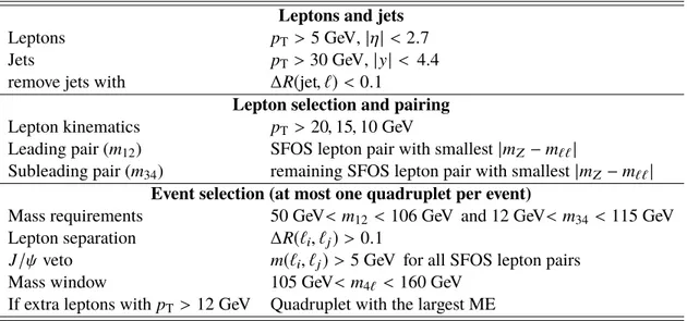
Table 2: List of event selection requirements which define the fiducial phase space for the cross section measurement.

SFOS lepton pairs are same-flavour opposite-sign lepton pairs.

Leptons and jets Leptons p

> 5 GeV, |η| < 2 . 7

Jets p

> 30 GeV, | y | < 4.4

remove jets with ∆R( jet , `) < 0 . 1

Lepton selection and pairing Lepton kinematics p

> 20 , 15 , 10 GeV

Leading pair ( m

) SFOS lepton pair with smallest |m

− m

|

Subleading pair ( m

) remaining SFOS lepton pair with smallest |m

− m

| Event selection (at most one quadruplet per event)

Mass requirements 50 GeV < m

< 106 GeV and 12 GeV < m

< 115 GeV Lepton separation ∆R(`

, `

) > 0 . 1

J /ψ veto m(`

, `

) > 5 GeV for all SFOS lepton pairs Mass window 105 GeV < m

< 160 GeV

If extra leptons with p

> 12 GeV Quadruplet with the largest ME

Using the same procedure as for reconstructed events, the selected dressed leptons are used to form quadruplets. In case of VH or ttH production, additional leptons not originating from a Higgs boson decay can induce a “lepton mispairing” when assigning them to the leading and subleading Z bosons. To improve the lepton pairing efficiency, the matrix-element-based pairing method as described in Section 4.2 is employed. The variables used in the differential cross section measurement are calculated using the dressed leptons of the quadruplets.

The acceptance of the fiducial selection, defined as the ratio of the number of events passing the particle-level selection and the events generated in a given bin or final state (with respect to the full phase space of H → Z Z

→ 2 ` 2 `

, where `, `

= e or µ ) is about 49% for a SM Higgs boson with m

= 125 GeV. The ratio C of the number of events passing the selection after detector simulation and event reconstruction to those passing the particle-level selection is about 45%. Due to resolution effects, about 1.6% of the events which pass the detector-level selection fail the particle-level selection.

6.1.2 Signal extraction and unfolding

To extract the number of signal events in each bin of a differential distribution (or for each decay final state for the inclusive fiducial cross section), invariant mass templates for the Higgs boson signal and the background processes are fit to the m

distribution in data. Compared to the previous analyses [11, 29] , the non-resonant Z Z background is fitted simultaneously with the signal and constrained by extending the m

fit range from 115-130 GeV to 105-160 GeV. For the total and fiducial cross sections in different final states, the same normalisation factor is used for the Z Z contribution. For the differential cross section measurements, multiple Z Z normalisation factors are introduced in the model4. The reducible background is estimated from dedicated control regions as described in Section 5 and its overall normalisation and

4 A different Z Z scaling factor is used for each observable bin unless the impact of its statistical uncertainty reaches 5% of the

total expected uncertainty for the expected cross section for that bin. In this case, neighbouring bins use the same normalisation

factor.

shape can vary within the associated systematic uncertainties. Finally, for the differential distributions, no split into decay final states is performed, and the SM Z Z

→ 4 ` decay fractions are assumed.

The number of expected events N

in each observable reconstruction bin i , expressed as function of m

, is given by

N

(m

) = Õ

j

r

· ( 1 + f

) · σ

· P(m

) · L + N

(m

) (1) with

σ

= σ

· A

· B (2)

where A

is the acceptance in the fiducial phase space and σ

the total cross section in fiducial bin j , L is the integrated luminosity, B is the branching ratio and N

(m

) is the background contribution. The index j runs over all observable bins in the fiducial phase space. P(m

) is the m

signal shape containing the fraction of events expected in each bin, taken from MC simulation. The terms r

represent the detector response matrix, created with signal simulated samples and averaged across the different production modes, corresponding to the probability that an event generated within the fiducial volume in the observable bin j is reconstructed in the bin i . Figure 1 shows the response matrix for the p

T

and N

observables. The detector response matrix allows to account for bin-to-bin migrations in the unfolding, and is different from the bin-by-bin correction factor technique used in the previous analyses [11, 12, 29]. The events

0.05 0.1 0.15 0.2 0.25 0.3 0.35 0.4 0.45 0.5

0.412 0.041 0.026 0.392 0.024

0.030 0.383 0.023 0.023 0.396 0.014

0.027 0.392 0.015 0.024 0.405 0.013

0.017 0.435 0.007 0.016 0.479

0.020 0.530 0.030 0.561

0-10 10-20 20-30 30-45 45-60 60-80 80-120 120-200 200-350 350-1000

[GeV] (reco)

4l

pT 0-10

10-20 20-30 30-45 45-60 60-80 80-120 120-200 200-350 350-1000

[GeV] (truth)l4 Tp

ATLAS Preliminary 13 TeV H → ZZ* → 4l

(a)

0.05 0.1 0.15 0.2 0.25 0.3 0.35 0.4 0.45 0.5

0.393 0.048

0.051 0.343 0.052 0.006

0.005 0.077 0.328 0.050

0.009 0.070 0.342

jets=0

N Njets=1 Njets=2 Njets>=3

(reco) Njets jets=0

N jets=1 N

jets=2 N

>=3 Njets

(truth)jetsN

ATLAS Preliminary 13 TeV H → ZZ* → 4l

(b)

Figure 1: Response matrices for (a) the transverse momentum of the four leptons p

T

and (b) the number of jets N

. Only bins with a value above 0.005 are shown.

that are reconstructed but do not fulfil the fiducial selection criteria are treated as background and the

normalisation of this contribution is fixed to be a fraction of the events that pass the fiducial selection

( f

). This ranges from 1.1% to 1.7% depending on the bin of the observable unfolded or final state.

For p

T

the migration matrix is almost diagonal, with a purity of the diagonal terms that ranges from 87%

at low p

T

where the p

T

bins are narrow to 97% at high p

T

with wider p

T

bins. For the N

observable the migrations are more relevant due to the jet energy resolution and the presence of pileup jets in the reconstructed events, bringing the purity of the diagonal term for N

≥ 3 down to 68%.

Inclusive and differential cross sections are measured by performing a binned maximum likelihood fit and using the profiled likelihood ratio test statistics to extract the uncertainty on each parameter of interest as described in Section 8.1.

6.2 Production mode cross sections

The Higgs boson couplings to heavy SM vector bosons ( W and Z ), top quarks and gluons are studied by measuring the cross sections for different production processes. To achieve this, the reconstructed Higgs boson candidate events are classified into twelve categories, each sensitive to a different Higgs boson production mechanism or production kinematic region. For simplicity, these kinematic regions are called

“production bins”. The event yield in each category serves as an observable. To improve the sensitivity of the production bin cross section measurements, NN based [125–127] discriminating observables are introduced in most of the categories. Finally, categories with events in the m

mass sidebands are formed to constrain the normalisation of backgrounds with prompt leptons, namely Z Z and t tV ¯ .

6.2.1 Simplified template cross sections

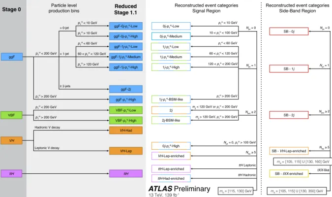
Theoretical uncertainties have a reduced impact on σ · B(H → Z Z

) results and enter primarily for the interpretation of the results in terms of Higgs boson couplings. The definitions of the production bins shown in the left hand-side panel of Figure 2 (shaded area) are based on particle-level events produced by dedicated event generators closely following the framework of Simplified Template Cross Sections [58, 128]. The bins are chosen in such a way that the precision of the measurement is maximised and at the same time possible Beyond Standard Model (BSM) contributions can be probed. All production bins are defined for Higgs bosons with rapidity |y

| < 2.5 and no requirements are placed on the particle-level leptons. Two sets of production bins are considered, with different granularity, as a trade-off between statistical and theoretical uncertainties.

For the first set (Stage 0) [58], production bins are simply defined according to the Higgs boson production mode: gluon–gluon fusion, vector boson fusion and associated production with vector bosons or top quark pairs. The bbH Higgs boson production bin is not included because there is insufficient sensitivity to measure this process with the current integrated luminosity. The bbH and ggF production modes have similar acceptance and their contributions are therefore considered together in the analysis, with their relative ratio fixed to the SM prediction. The sum of their contributions is referred to in the following as gluon–gluon fusion. Similarly, single top production ( tH ) is considered together with ttH , their relative ratio is fixed to the SM prediction. Differently from Stage 0 described in Ref. [58], the VH events with a hadronically decaying vector boson V are not included in the VBF bin.

For the second set (reduced Stage 1.1) [128], a more exclusive group of production bins is defined. This set is obtained by merging production bins of the Stage-1.1 set, a slightly updated version of that from Ref. [58], which cannot be measured separately in the H → Z Z

→ 4 ` channel with the current data sample. These bins are predominately defined using the Higgs boson transverse momentum ( p

T

) and

particle-level jets, which are built from all stable particles (all particles with c τ > 10 mm) including

ATLAS Preliminary

13 TeV, 139 fb^-1 Stage 0

VH VBF

ttH ggF

VH-Lep pT

H < 60 GeV

pTH > 120 GeV 60 < pTH < 120 GeV

≥ 2-jets

= 0-jet

= 1-jet

pT H > 200 GeV pTH < 200 GeV

Leptonic V decay Hadronic V decay

Reduced Stage 1.1

ttH ggF-0j-pTH-Low

ggF-1j-p_T^H-High ggF-1j-p_T^H-Low ggF-1j-p_T^H-Medium

ggF-0j-p_T^H-High

VH-Had VBF-p_T^H-Low VBF-p_T^H-High ggF-2j ggF-pTH-High p_T^H < 200 GeV

p_T^H > 200 GeV

pTH < 10 GeV pT

H > 10 GeV

Particle level production bins

m4l = [115, 130] GeV ttH Leptonic

N_lep ≥ 5 p_T^4l < 10 GeV

ttH Hadronic N_jet = 0, p_T^4l > 100 GeV 10 < p_T^4l < 100 GeV

60 < p_T^4l < 120 GeV pT

4l < 60 GeV

120 < p

T

4l < 200 GeV N_jet = 1 N_jet = 0

m_jj > 120 GeV, p_T^4l > 200 GeV mjj < 120 GeV or p

T 4l < 200 GeV p_T^4l > 200 GeV

N_jets ≥ 2

SB - 0j

N_jet = 1 N_jet = 0

SB - 1j

m4l = [105, 115] U [130, 350] GeV N_lep ≥ 5 N_jets ≥ 2

tXX-like SB - VH-Lep-enriched

SB - 2j

SB - tXX-enriched

m4l = [105, 115] U [130, 160] GeV Reconstructed event categories

Signal Region

Reconstructed event categories Side-Band Region

0j-pT4l-Low

1j-p_T^4l-Medium 1j-p_T^4l-High

ttH-Lep-enriched 2j 2j-BSM-like

ttH-Had-enriched 0j-p_T^4l-Medium

0j-pT4l-High VH-Lep-enriched

1j-p_T^4l-BSM-like 1j-pT

4l-Low

Figure 2: The phase-space regions (production bins) for the measurement of the Higgs boson production cross sections which are defined at the particle level for Stage 0 and reduced Stage 1.1 (left panel), and the corresponding reconstructed event categories for signal (middle panel) and sidebands (right panel). The description of the production bins is given in Section 6.2.1, while the reconstructed event categories are described in Section 6.2.2. The bbH ( tH ) contribution is included in the ggF ( ttH ) production bins.

neutrinos, photons and leptons from hadron decays or produced in the shower. All Higgs boson decay products, as well as the leptons and neutrinos from the decays of the signal V bosons are not included in the particle level jets, while the decay products from hadronically decaying signal V bosons are included.

The anti- k

jet reconstruction algorithm with a radius parameter R = 0 . 4 is used and jets are required to have p

> 30 GeV.5 The gluon–gluon fusion process is split into seven production bins: six have a Higgs boson transverse momentum below 200 GeV and are separated according to the number of jets (0, 1 and ≥ 2) and then according to p

T

; the seventh is a BSM bin with Higgs boson transverse momentum above 200 GeV. The p

T

splitting for the 0-jet bin is below and above 10 GeV, and for 1-jet below 60 GeV, between 60 GeV and 120 GeV, and above 120 GeV. In Stage 1.0, the BSM bin had been split into multiple jet bins. The 0-jet bin with p

T

above 10 GeV is also new to Stage 1.1, and captures the Z H production where the Z decays into neutrinos. The reduced Stage-1.1 gluon–gluon fusion bins are denoted by ggF-0 j - p

T

-Low, ggF-0 j - p

T

-High, ggF-1 j - p

T

-Low, ggF-1 j - p

T

-Med, ggF-1 j - p

T

-High, ggF-2 j and ggF- p

T

-High. The VBF production bin is split into two p

T

bins, below and above 200 GeV (VBF- p

T

-Low and VBF- p

T

-High, respectively). The former bin is expected to be dominated by SM events, while the latter is sensitive to potential BSM contributions. For VH production, separate bins with hadronically ( VH -Had) and leptonically ( VH -Lep) decaying vector bosons are considered. The leptonic V boson decays

5 The main difference in the particle jet definition for the differential cross section measurement and the production mode cross

section measurements is that hadronic taus decays from the vector bosons associated with the Higgs production are included in

the former and not in the latter.

include the decays into τ leptons and into neutrino pairs. Differently from Stage 1.1 the VH -Had is not included in the VBF. The ttH production bin remains the same as for Stage 0.

The central panel of Figure 2 summarises the corresponding categories of reconstructed events in which the cross section measurements are performed and which are described in more detail in Section 6.2.2.

There is a dedicated reconstructed event category for each production bin except for ggF-2 j , VBF- p

T

-Low and VH -Had. These production bins are largely measured from the 2-jet reconstruction category and to a lesser extent the 1-jet categories using the NN discriminants.

6.2.2 Categorisation of reconstructed Higgs boson event candidates

The classification of events is performed for both signal events with 115 GeV < m

< 130 GeV and background events in the mass sidebands. For signal events, this is performed in the following order. First, events are classified as enriched in the ttH process by requiring at least one b -tagged jet in the event (with 85% b -tagging efficiency). The ttH category is split according to the decay mode of the two W bosons from the top quark decays. For semi- and di-leptonic decays ( ttH -Lep-enriched), at least one additional lepton with p

> 12 GeV6 together with at least two b -tagged jets (with 85% b -tagging efficiency) or at least five jets with at least one b -tagged jet (with 85% b -tagging efficiency) or at least two jets with at least one b -tagged jet (with 60% b -tagging efficiency) is required. For the fully hadronic decay ( ttH -Had-enriched), there must be either at least five jets with at least two b -tagged jets (with 85% b -tagging efficiency) or at least four jets with at least one b -tagged jet (with 60% b -tagging efficiency). Events with additional leptons but not satisfying the above jet requirements define the next category enriched in VH production events with leptonic vector boson decays ( VH -Lep-enriched).

The remaining events are classified according to their jet multiplicity into events with no jets, exactly one jet or at least two jets. Events with at least two jets are divided into two categories: one is a BSM-like category (2 j -BSM-like) and the other (2 j ) contains the bulk of events with significant contributions from the VBF and VH production modes in addition to ggF. The 2 j -BSM-like category requires the invariant mass m

of the two leading jets to be larger than 120 GeV and the four-lepton transverse momentum, p

T

, larger than 200 GeV, the remaining events are classified in the 2 j category. Events with zero or one jet in the final state are expected to be dominated by the ggF process. Following the particle-level definition of production bins from Section 6.2.1, the 1-jet category is further split into four categories with p

T

smaller than 60 GeV (1 j - p

T

-Low), between 60 and 120 GeV (1 j - p

T

-Med), between 120 and 200 GeV (1 j - p

T

-High), and larger than 200 GeV (1 j - p

T

-BSM-Like). The largest number of ggF events and the highest ggF purity are expected in the zero-jet category (0 j ). The zero-jet category is split in three categories with p

T

smaller than 10 GeV (0 j - p

T

-Low), between 10 and 100 GeV (0 j - p

T

-Med) and above 100 GeV (0 j - p

T

-High). The first two categories follow the production bin splitting, and the last category improves the discrimination between VH ( V → `ν/νν ) and ggF.

The right-hand panel of Figure 2 shows the background event classification. For the ttH categories, there is a t X X -enriched sideband category (SB- t X X -enriched) which includes events with at least two jets including at least one tagged as a b-jet with 60% efficiency and E

T

> 100 GeV in the mass range 105-115 GeV or 130-350 GeV. This region is dominated by tt Z (87%) and has small contributions from: ttt , tttt , tW Z , ttW , ttWW , ttW Z , tt Z γ , tt Z Z , and t Z . This large mass range, larger than for the non-resonant Z Z discussed next, allows for an improved statistical precision on the estimation of this background. For the

6 The additional lepton is a lepton candidate as defined in Section 4.1, and is also required to satisfy the same isolation, impact

parameter and angular separation requirements as the leptons in the quadruplet.

non-resonant Z Z production, events not passing the criteria for SB- t X X -enriched category are split in the m

mass range 105-115 GeV or 130-160 GeV according to the number of reconstructed jets: zero jet (SB-0 j ), one jet (SB-1 j ) or ≥ 2 jets (SB-2 j ). Similarly, events in the same mass range with an extra reconstructed lepton form the SB- V H -Lep-enriched category.

The expected number of signal events is shown in Table 3 for each Stage-0 production bin and separately for each reconstructed event category. The ggF and bbH contributions are shown separately in order to compare their relative contributions, but both belong in the same (ggF) production bin. The highest bbH event yield is expected in the 0 j category since the jets tend to be more forward than in the ttH process, thus escaping the acceptance of the ttH selection criteria. The sources of uncertainty on these expectations are detailed in Section 7. The signal composition in terms of the reduced Stage-1.1 production bins is shown in Figure 3. The separation of the contributions from different production bins, such as the sizeable contribution of the ggF-2 j component in reconstructed categories with two or more jets, is further improved by means of NN observables, as described in the following.

Table 3: The expected number of SM Higgs boson events with m

= 125 GeV at an integrated luminosity of 139 fb

and

√ s = 13 TeV in each reconstructed event signal (115 < m

< 130 GeV) and sideband ( m

in 105-115 GeV or

130-160 GeV for Z Z

, 130-350 GeV for tXX ) category, shown separately for each Stage-0 production bin. The ggF and bbH yield are shown separately but both contribute to the same (ggF) production bin, and Z H and W H are reported separately but are merged together for the final result. Statistical and systematic uncertainties, including those for theory, are added in quadrature. Contributions that are below 0.2% of the total signal in each reconstructed category are not shown and replaced by “-”.

Reconstructed SM Higgs boson production mode

event category ggF VBF WH ZH ttH+ tH bbH

Signal 115<m_4`<130 GeV

0j-p^4`

T-Low 24.6±3.1 0.077±0.010 0.0194±0.0035 0.0131±0.0024 − 0.18±0.09 0j-p^4`

T-Med 76±8 1.18±0.14 0.39±0.05 0.36±0.04 − 0.8±0.4

0j-p^4`

T-High 0.132±0.032 0.0302±0.0033 0.064±0.006 0.161±0.015 0.00065±0.00025 − 1j-p^4`

T-Low 30±4 2.03±0.11 0.52±0.05 0.306±0.031 0.0074±0.0016 0.40±0.20 1j-p^4`

T-Med 17.5±2.8 2.65±0.16 0.52±0.05 0.354±0.035 0.0087±0.0020 0.09±0.05 1j-p^4`

T-High 3.7±0.8 0.93±0.07 0.167±0.014 0.154±0.013 0.0047±0.0011 0.012±0.006 1j-p^4`

T-BSM-Like 0.90±0.23 0.268±0.019 0.065±0.010 0.052±0.008 0.0017±0.0006 0.0008±0.0004 2j 23±5 8.0±0.5 1.86±0.14 1.44±0.11 0.47±0.05 0.28±0.14 2j-BSM-like 1.9±0.6 1.05±0.05 0.119±0.013 0.110±0.012 0.078±0.007 0.0027±0.0014 VH-Lep-enriched 0.046±0.017 0.0191±0.0031 0.80±0.06 0.211±0.017 0.172±0.015 0.0026±0.0013 ttH-Had-enriched 0.13±0.13 0.0162±0.0033 0.0142±0.0024 0.044±0.007 0.73±0.08 0.017±0.009 ttH-Lep-enriched 0.0008±0.0012 0.00019±0.00014 0.0039±0.0024 0.0023±0.0014 0.40±0.04 − Sideband 105<m_{4`</sub><115 GeV or 130<m<sub>4`}<160 GeV

SB-0j 4.4±0.5 0.058±0.009 0.103±0.012 0.040±0.005 − 0.046±0.024 SB-1j 2.30±0.29 0.256±0.023 0.100±0.011 0.060±0.006 0.0056±0.0012 0.021±0.011 SB-2j 1.17±0.25 0.40±0.05 0.116±0.014 0.089±0.010 0.109±0.010 0.016±0.008 SB-V H-Lep-enriched 0.019±0.008 0.0029±0.0010 0.086±0.008 0.090±0.008 0.066±0.007 0.0013±0.0007

105<m_{4`</sub><115 GeV or 130<m<sub>4`}<350 GeV

SB-t X X-enriched 0.0009±0.0015 0.00015±0.00015 0.00042±0.00016 0.00041±0.00016 0.064±0.008 0.00008±0.00008 Total 186±14 17.0±0.8 5.0±0.4 3.48±0.25 2.12±0.18 1.9±1.0

Expected Composition

-Lep-enriched ttH

-Had-enriched ttH

-High

4l

pT

- j 0

-Lep-enriched VH

-BSM-Like 2j

2j -BSM-Like

4l

pT

- j 1

-High

4l

pT

- j 1

4l-Med pT

- j 1

4l-Low pT

- j 1

4l-Med pT

- j 0

4l-Low pT

- j 0

Reconstructed Event Category

0 0.1 0.2 0.3 0.4 0.5 0.6 0.7 0.8 0.9 1

H-Low pT

- j ggF-0

-High

H

pT

- j ggF-0

H-Low pT

- j ggF-1

H-Med pT

- j ggF-1

-High

H

pT

- j ggF-1 j ggF-2

-High

H

pT

ggF-

H Low VBF-pT

High

H

VBF-pT

-Had VH

-Lep VH

tH + ttH

ATLAS Simulation Preliminary

4l ZZ* → H →

13 TeV, 139 fb-1

Figure 3: Standard Model signal composition in terms of the reduced Stage-1.1 production bins in each reconstructed event category. The bbH contributions are included in the ggF production bins.

6.2.3 Discriminating observables

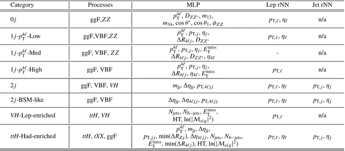
In order to further increase the sensitivity of the cross section measurements in the production bins (Section 6.2.1), NN discriminants are introduced in the reconstructed event categories as part of the fit procedure. The NNs are trained on simulated SM Higgs boson signal and non-Higgs background or the other production processes, based on several discriminating observables. Two types of neural networks are used: feed-forward, or a multilayer percepton (MLP), and recurrent (rNN) [125–127]. Each NN combines two rNNs, one for the four leptons and one for up to three jets, and an MLP with additional variables. The rNNs are exclusively trained to capture the the relevant properties of the different production modes. These three components, MLP and two rNNs, are chained into another MLP to complete a NN. Each category uses a NN to discriminate between two or three processes, e.g. ggF, VBF and Z Z background, where the NN is configured to have an output for the posterior probability of each process. The variables used for training the MLP and rNNs for each category along with the processes being separated are summarised in Table 4.

The variables entering the NN training listed in Table 4, which have not been previously described in

this note are as follows. The kinematic discriminant D

[129], defined as the difference between the

logarithms of the signal decay (same as in Section 4.2) and background matrix elements ( M

and M

respectively) squared, is used to distinguish ggF from the non-resonant Z Z background, as well as three

angles [130]: the leading Z boson production angle θ

in the four-lepton rest frame, the angle θ

between

the negatively charged lepton of the leading Z in the leading Z rest frame and the direction of flight of the

leading Z in the four-leptons rest frame, and the angle φ

between two Z decay planes in the four lepton

rest frame. The angular separation of a jet from the 4 ` system, ∆R

, is used to distinguish VBF or ttH

Table 4: The input variables used to train the MLP, and the two rNNs for the four leptons and the jets (up to three).

For each category, the processes which are classified by a NN and their corresponding variables are shown. For example, there are eight variables for the Lep rNN being trained if p

and η

are listed. Leptons and jets are denoted by “ ` ” and “ j ”. See the text for variable definitions.

Category Processes MLP Lep rNN Jet rNN

0j ggF,Z Z p^4`

T,DZ Z^∗,m₁₂, pT,`,η` n/a

m₃₄, cosθ^∗, cosθ₁,φZ Z

1j-p^4`

T-Low ggF,VBF,Z Z ∆Rp<sup>4`</sup><sub>T4`j</sub>,p,T,jD,Z Zηj^∗, p_{T,`</sub>,η<sub>`} n/a 1j-p^4`

T-Med ggF, VBF,Z Z p^4`

T,pT,j,ηj,E^miss

T - n/a

∆R<sub>4`</sub>j,DZ Z<sup>∗</sup>,η4`

1j-p^{4`</sup><sub>T</sub>-High ggF, VBF p<sup>4`}

T,p_T,j,ηj, pT,` n/a

∆R_{4`</sub>j,η<sub>4`},E^miss

T

2j ggF, VBF,VH m_jj,∆η_jj,p_{T,4`</sub>j j p<sub>T,`},η_` p_T,j,ηj

2j-BSM-like ggF, VBF ∆η_jj,∆η4`j j,pT,4`j j pT,`,η` pT,j,ηj

VH-Lep-enriched ttH,VH N_jets,Nb−jets,E^miss

T , pT,` n/a

HT, ln(|M_sig|²) ttH-Had-enriched ttH,tXX, ggF

p^4`_T,m_jj,∆η_jj,

p_{T,`</sub>,η<sub>`} p_T,j,ηj

pT,j j, min(∆R_{Z j}),∆η4`j j,N_jets,Nb−jets, E^miss

T , min(∆R_4`j), HT, ln(|Msig|²)

from ggF. For categories with two or more jets, the kinematic variables of the two leading jets are used, e.g.

invariant mass, m

, separation in η , ∆η

, transverse momentum, p

, or in relation to the 4 ` system, i.e.

p

or ∆ η

. For the ttH -Had-enriched category, the number of jets, N

, and b-tagged jets, N

, are used. HT is the scalar sum of all vectors entering the E

T

calculation. Finally, ln (|M

|

) is used for the VH -Lep-enriched and ttH -Had-enriched categories.

Depending on the category and the number of processes being targeted, the NN has two or three output

nodes. The value computed at each node represents the probability, with an integral of one, for the event

to originate from the given process. For example, for the 0-jet category, two probabilities are evaluated,

NN

and NN

. As these two values are a linear transformation of each other, only one output, NN

,

is used as a discriminant in the fit model. In categories with three targeted processes, only two output

probabilities are independent. To incorporate these into the fit model, the events in this category are divided

into two sub-categories and one of two output probabilities is used in each sub-category. For example, in

the 1-jet category, NN

and NN

are used. The sub-categories are defined by requiring NN

to be

smaller or larger than 0.25. In these two regions, NN

and NN

probabilities are used respectively as

discriminant in the fit model.