Measurement of the Higgs boson decaying to

A TLAS-CONF-2020-058 06 November 2020

ATLAS CONF Note

ATLAS-CONF-2020-058

29th October 2020

Measurement of the Higgs boson decaying to b -quarks produced in association with a top-quark

pair in p p collisions at √

s = 13 TeV with the ATLAS detector

The ATLAS Collaboration

The associated production of a Higgs boson with a top-quark pair is measured in events characterised by the presence of one or two electrons or muons. The Higgs boson decay into a b -quark pair is considered. The analysed data, corresponding to an integrated luminosity of 139 fb

, were collected in proton–proton collisions at the Large Hadron Collider between

2015 and 2018 at a centre-of-mass energy of

√ s = 13 TeV. The measured signal strength, defined as the ratio of the measured signal yield to that predicted by the Standard Model, is 0 . 43

. This result corresponds to an observed (expected) significance of 1.3 (3.0) standard deviations, in agreement with the Standard Model prediction. For the first time, the signal strength is measured differentially in bins of the Higgs boson transverse momentum in the simplified template cross-section framework, including a boosted selection targeting Higgs boson transverse momentum above 300 GeV.

© 2020 CERN for the benefit of the ATLAS Collaboration.

Reproduction of this article or parts of it is allowed as specified in the CC-BY-4.0 license.

1 Introduction

The Higgs boson [1–3] was discovered by the ATLAS and CMS collaborations [4, 5] in 2012, with a mass of around 125 GeV [6]. Since then, the analysis of proton–proton ( pp ) collision data at centre-of-mass energies of 7 TeV, 8 TeV and 13 TeV delivered by the Large Hadron Collider (LHC) [7] has led to more detailed measurements of its properties and couplings, testing the predictions of the Standard Model (SM).

Of particular interest is the Yukawa coupling to the top quark, the heaviest elementary particle in the SM, which could be very sensitive to effects of physics beyond the SM (BSM) [8].

Both the ATLAS and CMS collaborations have observed the interaction of the Higgs boson with third- generation fermions of the SM. The coupling to τ -leptons was measured in the observation of H → ττ decays [9, 10], while the observation of the decay of the Higgs boson into b -quark pairs provided direct evidence for the Yukawa coupling to down-type quarks [11, 12]. The interaction of the Higgs boson with the top quark was measured in the observation of Higgs boson production in association with a pair of top quarks ( t¯ tH ) [13, 14].

The t tH ¯ production mode is the most favourable for a direct measurement of the top-quark Yukawa coupling without assumptions on the potential presence of BSM physics [15–18]. Although this production mode only contributes around 1% of the total Higgs-boson production cross-section [19], the top quarks in the final state offer a distinctive signature and allow access to many Higgs boson decay modes. The decay to two b -quarks ( H → b b ¯ ) is the most probable, with a SM branching fraction of about 58% [19]. Furthermore, in the H → b b ¯ decay mode the reconstruction of the Higgs boson kinematics is possible, which allows the extraction of additional information on the structure of the top–Higgs interaction [20–23]. This analysis therefore aims at selecting events with a Higgs boson produced in association with a pair of top quarks and decaying to a pair of b -quarks t¯ tH(b b) ¯

, in which one or both top quarks decay semi-leptonically, producing an electron or a muon, collectively referred to as leptons ( ` ).

With many final-state particles, the main challenges are the low efficiency to reconstruct and identify all of them, the large combinatorial ambiguities when associating the observed decay products to the Higgs boson and top quarks, and the large background of tt+jets processes, in particular when these jets originate from b - or c -quarks, which have a much larger production cross-section than the signal.

The ATLAS collaboration searched for t¯ tH(b b) ¯ production at

√ s = 8 TeV in final states with at least one [24] or no lepton [25], and at

√ s = 13 TeV with at least one lepton in the final state with data collected in 2015 and 2016, corresponding to an integrated luminosity of 36.1 fb

[26]. A combined signal strength of 0 . 84

0.61

was measured, with an observed (expected) significance of 1.4 (1.6) standard deviations.

This result was combined with analyses of Higgs boson decays to massive vector bosons, τ -leptons, or photons to claim observation of the t tH ¯ production mode [13]. The CMS collaboration searched for the same processes using data collected in 2016, corresponding to an integrated luminosity of 35.9 fb

at

√ s = 13 TeV, with at least one lepton [27] or no lepton [28], which measured a signal strength of 0 . 72 ± 0 . 45 and 0 . 9 ± 1 . 5, respectively. These results also contributed to the observation of the t tH ¯ production mode [14].

In this note, a measurement of the t¯ tH production cross-section in the H → b b ¯ channel is performed using the LHC Run 2 pp collision data collected by the ATLAS detector, corresponding to an integrated luminosity of 139 fb

at

√ s = 13 TeV. The analysis targets Higgs bosons decaying to b -quarks which account for at least 94% of t¯ tH events selected in the signal regions, but all the decay modes are considered and may contribute to the signal. Events with either one (single-lepton) or two (dilepton) leptons are

1

Electrons and muons from the decay of a τ-lepton itself originating from a W boson are included.

analysed separately in exclusive categories according to the number of leptons, the number of jets and the number of jets originating from b -hadrons ( b -jets). In the single-lepton channel, a specific category, referred to as ‘boosted’ in the following, is designed to select events in which the Higgs boson is produced with high transverse momentum ( p

). The non-boosted categories are referred to as ‘resolved’. Machine learning algorithms are used to classify events in signal-rich categories, which are analysed together with the signal-depleted ones in a combined profile likelihood fit. The output distributions of these multivariate algorithms are used as the main discriminant to extract the signal. This signal extraction fit simultaneously determines the event yields for the signal and for the most important background components, while constraining the overall background model within the assigned systematic uncertainties. In addition, making use of the possibility to reconstruct the Higgs boson kinematics in the H → b b ¯ channel, the cross-section is measured as a function of the Higgs boson transverse momentum p

T

in the simplified template cross-sections (STXS) formalism [19], which aims to separate measurement and interpretation steps in order to reduce the theory dependencies that are folded into the measurements.

This note is organised as follows. The ATLAS detector is described in Section 2. The signal and background modelling is presented in Section 3. Section 4 summarises the selection criteria for reconstructed objects and events, while Section 5 describes the analysis strategy. Systematic uncertainties are discussed in Section 6. Results are presented in Section 7, and the conclusions in Section 8.

2 ATLAS detector

The ATLAS experiment [29–31] at the LHC is a multi-purpose particle detector with a forward-backward symmetric cylindrical geometry and a near 4 π coverage in solid angle.

It consists of an inner tracking detector surrounded by a thin superconducting solenoid providing a 2 T axial magnetic field, electromagnetic and hadron calorimeters, and a muon spectrometer. The inner tracking detector (ID) covers the pseudorapid- ity range |η| < 2 . 5. It consists of silicon pixel, silicon microstrip, and transition radiation tracking detectors.

Lead/liquid-argon (LAr) sampling calorimeters provide electromagnetic (EM) energy measurements with high granularity. A hadron steel/scintillator-tile calorimeter covers the central pseudorapidity range

|η| < 1 . 7. The end-cap and forward regions are instrumented with LAr calorimeters for both EM and hadronic energy measurements up to |η| = 4 . 9. The muon spectrometer surrounds the calorimeters and is based on three large air-core toroidal superconducting magnets with eight coils each. The field integral of the toroids ranges between 2 and 6 T m across most of the detector. The muon spectrometer includes a system of precision tracking chambers and fast detectors for triggering. A two-level trigger system is used to select events. The first-level trigger is implemented in hardware and uses a subset of the detector information to accept events at a rate below 100 kHz. This is followed by a software-based trigger that reduces the accepted event rate to 1 kHz on average depending on the data-taking conditions [32].

2

ATLAS uses a right-handed coordinate system with its origin at the nominal interaction point (IP) in the centre of the detector and the z -axis along the beam pipe. The x -axis points from the IP to the centre of the LHC ring, and the y -axis points upwards.

Cylindrical coordinates ( r, φ ) are used in the transverse plane, φ being the azimuthal angle around the z -axis. The pseudorapidity is defined in terms of the polar angle θ as η = − ln tan (θ/ 2 ) . Angular distance is measured in units of ∆R ≡ p

(∆η)

+ (∆φ)

.

3 Signal and background modelling

Simulation is used to model the t tH ¯ signal and the background processes. The rate and shape of variables selected to discriminate between signal and background provide distributions which enter into the signal extraction fit, which also constrains the modelling of the background processes. In this analysis, the Monte Carlo (MC) samples were simulated either using the full ATLAS detector simulation [33] based on Geant4 [34] or with a faster simulation where the full Geant4 simulation of the calorimeter response is replaced by a detailed parameterisation of the shower shapes [33]. For the observables used in this analysis, both simulations were found to give similar modelling. To simulate the effects of multiple interactions in the same and neighbouring bunch crossings (pileup), additional interactions were generated using Pythia8.186 [35] with the A3 set of tunable parameters [36] and overlaid onto the simulated hard-scatter event. Simulated events are reweighted to match the pileup conditions observed in the full Run 2 data, with a mean number of pp interactions per bunch crossing of 34. All simulated events are processed through the same reconstruction algorithms and analysis chain as the data.

In all MC samples for which the parton shower (PS), hadronisation, and multi-parton interaction (MPI) are generated either with Pythia8 or Herwig7 [37, 38], the decays of b - and c -hadrons are simulated using the EvtGen v1.6.0 program [39]. The b -quark mass is set to m

= 4 . 80 GeV (4 . 50 GeV) for samples using Pythia8 (Herwig7). For Pythia8, the A14 [40] set of parameters is used, with the NNPDF2.3LO parton distribution function (PDF) set [41]. For Herwig7, the H7UE set of tuned parameters [38] is used with the MMHT2014LO PDF set [42]. The Higgs boson mass is set to m

= 125 . 0 GeV, and the top-quark mass to m

= 172.5 GeV. A summary of all generated samples is presented in Table 1, which includes both the nominal predictions and other samples used to assess systematic uncertainties.

3.1 Signal modelling

The production and decay of t tH ¯ events is modelled in the five-flavour scheme using the PowhegBox [58–62]

generator at next-to-leading order (NLO) in quantum chromodynamics (QCD) with the NNPDF3.0NLO [63]

PDF set. The h

parameter

is set to 0 . 75 × (m

+ m

+ m

) = 352 . 5 GeV, and the functional form of the renormalisation and factorisation scales are both set to

p m

(t) · m

( t) · ¯ m

(H) (with m

= q

m

+ p

T

the transverse mass of a particle). The events are showered with Pythia8 and all Higgs-boson decay modes are considered. The samples are normalised to the fixed-order calculation, σ

= 507 fb, which includes NLO QCD and electroweak (EW) corrections [19].

3.2 t t ¯ + jets background

Simulated t t ¯ + jets events are categorised according to the flavour of additional jets in the event, using the procedure described in Ref. [24]. Jets are reconstructed from stable particles (mean lifetime τ > 3 × 10

s) using the anti- k

algorithm [64, 65], and the number of b - or c -hadrons within ∆R < 0 . 4 of the jet axis is considered, excluding particles produced from the top-quark decay. Events are labelled as t¯ t + ≥ 1 b if at least one b -flavour jet is identified, t t ¯ + ≥ 1 c if at least one c -flavour jet is identified, and otherwise as t¯ t + light. The t¯ t + ≥ 1 b events may be further split in subcomponents: t t ¯ + 1 b/ 1 B and t¯ t + ≥ 2 b , where 1 b

3

The h

parameter controls the p

of the first additional emission beyond the leading-order Feynman diagram in the PS and

therefore regulates the high- p

emission against which the t¯ t system recoils.

means only one jet is matched to a b -hadron, 1 B that exactly one jet is matched to two or more b -hadrons, and the remaining events are labelled as t t ¯ + ≥ 2 b .

To accurately model the dominant t¯ t + ≥ 1 b background, a sample with t¯ t + b b ¯ matrix elements (ME) was produced at NLO QCD accuracy in the four-flavour scheme with the PowhegBoxRes [66] generator and OpenLoops [67, 68], using a pre-release of the implementation of this process in PowhegBoxRes provided by the authors [69], with the NNPDF3.0NLOnf4 [63] PDF set, and using Pythia8 for the PS and hadronisation. The factorisation scale is set to 0 . 5 × Σ

t,b,¯ b,¯j

m

(i) (where j stands for extra partons), the renormalisation scale is set to

p m

(t) · m

(¯ t) · m

(b) · m

( b) ¯ , and the h

parameter is set to 0 . 5 × Σ

m

(i) . The mass of the two b -quarks produced in the ME in association with the two top quarks is set to the same value as the mass of the b -quarks from the top-quark decays, m

= 4 . 95 GeV.

Inclusive t t ¯ + jets events are also generated in the five-flavour scheme using the PowhegBox v2 generator at NLO in QCD, using Pythia8 for the PS and hadronisation. Here, the h

parameter is set to 1.5 m

[44], and the functional form of the renormalisation and factorisation scales is set to m

(t) .

The t¯ t + ≥ 1 c and t¯ t + light events using this prediction are combined with the previously described t¯ t + ≥ 1 b sample to form the nominal t t ¯ model, while the t t ¯ + ≥ 1 b events from this five-flavour scheme are used only to assign a subset of modelling uncertainties.

3.3 Other backgrounds

The QCD V + jets processes (i.e. W + jets and Z + jets) are simulated with the Sherpa v2.2.1 generator [70].

In this setup, NLO-accurate ME for up to two partons, and leading-order (LO) accurate ME for up to four partons are calculated with the Comix [71] and OpenLoops libraries. They are matched with the Sherpa parton shower [72] using the MEPS@NLO prescription [73–76] with the set of tuned parameters developed by the Sherpa authors based on the NNPDF3.0NNLO set of PDFs [63]. A data-driven correction was derived for Z + jets predictions containing at least two heavy-flavour jets (where heavy-flavour means jets originating from b -hadrons and c -hadrons). Events were selected, with objects passing the selection discussed in Section 4, in dedicated control regions in data defined by requiring at least two jets and two opposite-electric-charge same-flavour leptons ( e

e

or µ

µ

) with an invariant mass inside the Z -boson mass window 83–99 GeV. A 25% yield increase was found to improve the modelling of Z + jets events with at least two heavy-flavour jets.

Diboson samples are simulated with the Sherpa v2.2 generator. In this setup multiple ME are matched and merged with the Sherpa PS based on the Catani-Seymour dipole factorisation [71, 72] using the MEPS@NLO prescription. For semi-leptonically and fully leptonically decaying diboson samples, as well as loop-induced diboson samples, the virtual QCD correction for ME at NLO accuracy is provided by the OpenLoops library. For electroweak VV j j production, the calculation is performed in the G

scheme, ensuring an optimal description of pure electroweak interactions at the electroweak scale. All samples are generated using the NNPDF3.0NNLO PDF set, along with the dedicated set of tuned PS parameters developed by the Sherpa authors.

4

This scale is calculated in the t t ¯ rest-frame and hence the p

of the top or anti-top quark is equivalent.

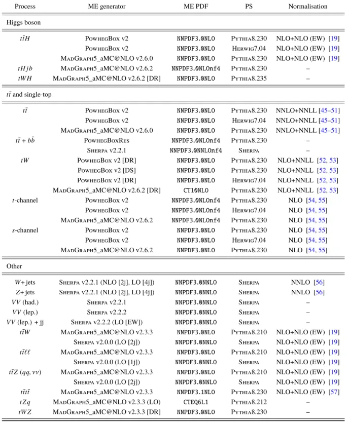
Table 1: Table summarising the generator setups used for MC samples in this analysis. The first row for each sample details the nominal settings used for this process in the analysis. For overlap between t t ¯ and tW -like diagrams, samples using the diagram removal scheme [43] are listed as [DR] and samples using the diagram subtraction scheme [43, 44]

are listed as [DS]. The precision of the matrix element (ME) generator is NLO in QCD if no additional information is provided in parentheses. The higher-order cross-section used to normalise these samples is listed in the last column and refers to the order of QCD processes if no additional information is provided. If no information is present in this column, there is no higher-order k -factor applied to this process. For the VV Sherpa samples, ‘lep.’ (‘had.’) means that both bosons decay leptonically (one decays leptonically and one hadronically).

Process ME generator ME PDF PS Normalisation

Higgs boson

t tH ¯ PowhegBox v2 NNPDF3.0NLO Pythia8.230 NLO+NLO (EW) [19]

PowhegBox v2 NNPDF3.0NLO Herwig7.04 NLO+NLO (EW) [19]

MadGraph5_aMC@NLO v2.6.0 NNPDF3.0NLO Pythia8.230 NLO+NLO (EW) [19]

tH j b MadGraph5_aMC@NLO v2.6.2 NNPDF3.0NLOnf4 Pythia8.230 –

tW H MadGraph5_aMC@NLO v2.6.2 [DR] NNPDF3.0NLO Pythia8.235 –

t¯ t and single-top

t¯ t PowhegBox v2 NNPDF3.0NLO Pythia8.230 NNLO+NNLL [45–51]

PowhegBox v2 NNPDF3.0NLO Herwig7.04 NNLO+NNLL [45–51]

MadGraph5_aMC@NLO v2.6.0 NNPDF3.0NLO Pythia8.230 NNLO+NNLL [45–51]

t¯ t + b b ¯ PowhegBoxRes NNPDF3.0NLOnf4 Pythia8.230 –

Sherpa v2.2.1 NNPDF3.0NNLOnf4 Sherpa –

tW PowhegBox v2 [DR] NNPDF3.0NLO Pythia8.230 NLO+NNLL [52, 53]

PowhegBox v2 [DS] NNPDF3.0NLO Pythia8.230 NLO+NNLL [52, 53]

PowhegBox v2 [DR] NNPDF3.0NLO Herwig7.04 NLO+NNLL [52, 53]

MadGraph5_aMC@NLO v2.6.2 [DR] CT10NLO Pythia8.230 NLO+NNLL [52, 53]

t -channel PowhegBox v2 NNPDF3.0NLOnf4 Pythia8.230 NLO [54, 55]

PowhegBox v2 NNPDF3.0NLOnf4 Herwig7.04 NLO [54, 55]

MadGraph5_aMC@NLO v2.6.2 NNPDF3.0NLOnf4 Pythia8.230 NLO [54, 55]

s -channel PowhegBox v2 NNPDF3.0NLO Pythia8.230 NLO [54, 55]

PowhegBox v2 NNPDF3.0NLO Herwig7.04 NLO [54, 55]

MadGraph5_aMC@NLO v2.6.2 NNPDF3.0NLO Pythia8.230 NLO [54, 55]

Other

W + jets Sherpa v2.2.1 (NLO [2j], LO [4j]) NNPDF3.0NNLO Sherpa NNLO [56]

Z + jets Sherpa v2.2.1 (NLO [2j], LO [4j]) NNPDF3.0NNLO Sherpa NNLO [56]

VV (had.) Sherpa v2.2.1 NNPDF3.0NNLO Sherpa –

VV (lep.) Sherpa v2.2.2 NNPDF3.0NNLO Sherpa –

VV (lep.) + jj Sherpa v2.2.2 (LO [EW]) NNPDF3.0NNLO Sherpa –

t¯ tW MadGraph5_aMC@NLO v2.3.3 NNPDF3.0NLO Pythia8.210 NLO+NLO (EW) [19]

Sherpa v2.0.0 (LO [2j]) NNPDF3.0NNLO Sherpa NLO+NLO (EW) [19]

t¯ t`` MadGraph5_aMC@NLO v2.3.3 NNPDF3.0NLO Pythia8.210 NLO+NLO (EW) [19]

Sherpa v2.0.0 (LO [1j]) NNPDF3.0NNLO Sherpa NLO+NLO (EW) [19]

t t Z ¯ (qq, νν) MadGraph5_aMC@NLO v2.3.3 NNPDF3.0NLO Pythia8.210 NLO+NLO (EW) [19]

Sherpa v2.0.0 (LO [2j]) NNPDF3.0NNLO Sherpa NLO+NLO (EW) [19]

t tt ¯ t ¯ MadGraph5_aMC@NLO v2.3.3 NNPDF3.1NLO Pythia8.230 NLO+NLO (EW) [57]

t Z q MadGraph5_aMC@NLO v2.3.3 (LO) CTEQ6L1 Pythia8.212 –

MC samples for associated production of a single top quark and a Higgs boson are also used. Two sub-processes, tH j b and tW H production, are generated using the MadGraph5_aMC@NLO v2.6.2 generator at NLO in QCD. The functional form of the renormalisation and factorisation scale is set to 0 . 5 × Í

i

m

(i) , where the sum runs over all the particles generated from the ME calculation. For tH j b ( tW H ), events are generated in the four- (five-) flavour scheme using the NNPDF3.0NLOnf4 ( NNPDF3.0NLO ) PDF set.

Single-top t - and s -channel, and tW production is modelled using the PowhegBox v2 [77–79] generator at NLO in QCD. For t -channel production, events are generated in the four-flavour scheme with the NNPDF3.0NLOnf4 PDF set, and the functional form of the renormalisation and factorisation scale is set to m

(b) following the recommendation of Ref. [77]. For s -channel and tW production, events are generated in the five-flavour scheme with the NNPDF3.0NLO PDF set, and the functional form of the renormalisation and factorisation scale is set to the top-quark mass. For tW production, the diagram removal scheme [43]

was employed to handle the interference with t¯ t production [44]. An additional sample which applies the diagram subtraction scheme [43, 44] was used to provide an uncertainty on the modelling of this interference.

The production and decay of a top-quark pair in association with a vector boson (i.e. t¯ tW or t¯ t Z ), referred to collectively as t¯ tV , is modelled using the MadGraph5_aMC@NLO v2.3.3 generator at NLO in QCD.

The functional form of the renormalisation and factorisation scale is set to 0 . 5 × Í

i

m

(i) , where the sum runs over all the particles generated from the ME calculation.

The production and decay of events with four top quarks is modelled using the MadGraph5_aMC@NLO v2.3.3 generator at NLO in QCD with the NNPDF3.1NLO [63] PDF set. The functional form of the renormalisation and factorisation scales are set to 0 . 25 × Í

i

m

(i) , where the sum runs over all the particles generated from the ME calculation, following the recommendation of Ref. [57].

The t Z q MC samples are generated using the MadGraph5_aMC@NLO v2.3.3 generator in the four-flavour scheme at LO in QCD, with the CTEQ6L1 [80] PDF set. Following the recommendations of Ref. [77], the renormalisation and factorisation scales are set to 4 × m

(b) , where the b quark is the one coming from the gluon splitting.

The tW Z sample is simulated using the MadGraph5_aMC@NLO v2.3.3 generator at NLO in QCD with the NNPDF3.0NLO PDF set. The renormalisation and factorisation scales are set to the top-quark mass. The diagram removal scheme is employed to handle the interference between tW Z and t t Z ¯ .

In the single-lepton channel, it was found that there is a negligible contribution from non-prompt lepton backgrounds, referred to as fakes, where either a jet is incorrectly reconstructed as a lepton, or where a dilepton process has a lepton outside of acceptance or not reconstructed. In the dilepton channel, the contribution of non-prompt lepton processes is very small and is estimated from simulation with a truth-level matching which only uses true dilepton events, with all remaining events being placed into a non-prompt lepton category.

In this analysis, some samples are merged to aid the stability of the signal extraction fit. Where a sample is

defined as ‘Other’, it contains the remaining processes not explicitly listed.

4 Object and event selection

Events are selected from pp collisions at

√ s = 13 TeV recorded by the ATLAS detector between 2015 and 2018, corresponding to an integrated luminosity of 139 fb

. Only events for which the LHC beams were in stable-collision mode and all relevant subsystems were operational are considered. Events are required to have at least one primary vertex with two or more tracks with p

> 0 . 5 GeV. If more than one vertex is found, the hard scattering primary vertex is selected as the one with the highest sum of squared transverse momenta of associated tracks [81].

Events were recorded using single-lepton triggers with either a low p

threshold and a lepton isolation requirement, or a higher threshold but a looser identification criterion and without any isolation requirement.

The lowest p

threshold at trigger level used for muons is 20 (26) GeV, while for electrons the threshold is 24 (26) GeV for the data taken in 2015 (2016–2018) [32].

Electrons are reconstructed from tracks in the ID associated with topological clusters of energy depositions in the calorimeter [82] and are required to have p

> 10 GeV and |η| < 2 . 47. Candidates in the calorimeter barrel–endcap transition region (1 . 37 < |η| < 1 . 52) are excluded. Electrons must satisfy the Medium likelihood identification criterion [83]. Muon candidates are identified by matching ID tracks to full tracks or track segments reconstructed in the muon spectrometer, using the Loose identification criterion [84].

Muons are required to have p

> 10 GeV and |η| < 2 . 5. Lepton tracks must match the primary vertex of the event, i.e. they have to satisfy |z

sin (θ)| < 0 . 5 mm and |d

/σ(d

)| < 5 ( 3 ) for electrons (muons), where z

is the longitudinal impact parameter relative to the primary vertex and d

(with uncertainty σ(d

) ) is the transverse impact parameter relative to the beam line.

Jets are reconstructed from noise-suppressed topological clusters of calorimeter energy depositions [85]

calibrated at the electromagnetic scale [86], using the anti- k

algorithm with a radius parameter of 0.4.

These are referred to as small- R jets. The average energy contribution from pileup is subtracted according to the jet area and jets are calibrated as described in Ref. [86] with a series of simulation-based corrections and in situ techniques. Jets are required to satisfy p

> 25 GeV and |η | < 2 . 5. The effect of pileup is reduced by an algorithm requiring that the calorimeter-based jets are validated as originating from the primary vertex using tracking information [87].

Jets originating from b -hadrons are identified ( b -tagged) with the MV2c10 multivariate algorithm [88]

which combines information from the impact parameter of displaced tracks as well as topological properties of secondary and tertiary decay vertices reconstructed within the jet. Four working points, defined by different thresholds on the MV2c10 discriminant, are used in this analysis, corresponding to an average efficiency ranging from 85% to 60% for b -jets with p

> 20 GeV as determined in simulated t t ¯ events. The corresponding rejection rates are in the range 2–22 for c -jets (originating from c -hadrons) and 27–1150 for light-jets (originating from light quarks and gluons). Jets are then assigned a pseudo-continuous b -tagging value according to the tightest working point they satisfy (pseudo-continuous b -tagging [88]). Correction factors are applied to the simulated events to compensate for differences between data and simulation in the b -tagging efficiency for b - [88], c - [89] and light-jets [90].

Hadronically decaying τ -leptons ( τ

) are distinguished from jets using their track multiplicity and a

multivariate discriminant based on calorimetric shower shapes and tracking information [91]. They are

required to have p

> 25 GeV, |η | < 2 . 5 and pass the Medium τ -identification working point.

An overlap removal procedure is applied to prevent double-counting of objects. The closest jet within

∆R

= p

(∆ y )

+ (∆φ)

= 0 . 2 of a selected electron is removed.

If the nearest jet surviving that selection is within ∆R

= 0 . 4 of the electron, the electron is discarded. Muons are usually removed if they are separated from the nearest jet by ∆R

< 0 . 4, which reduces the background from heavy-flavour decays inside jets. However, if this jet has fewer than three associated tracks, the muon is kept and the jet is removed instead; this avoids an inefficiency for high-energy muons undergoing significant energy loss in the calorimeter. A τ

candidate is rejected if it is separated by ∆R

< 0 . 2 from any selected electron or muon.

The missing transverse momentum (with magnitude E

T

) is reconstructed as the negative vector sum of the p

of all the selected electrons, muons, τ

and jets described above, with an extra ‘soft term’ built from additional tracks associated to the primary vertex, to make it resilient to pileup contamination [92].

The missing transverse momentum is not used for event selection but is included in the inputs to the multivariate discriminants that are built in the most sensitive analysis categories (see Section 5).

For the boosted category, the small- R jets are reclustered [93] using the anti- k

algorithm with a radius parameter of 1.0, resulting in a collection of large- R jets (referred to as RC jets). These RC jets are required to have a reconstructed invariant mass higher than 50 GeV, p

> 200 GeV and at least two small- R constituent jets. RC jets are used to identify top-quark and Higgs-boson candidates with high p

(boosted) and decaying into collimated hadronic final states. A deep neural network (DNN) with a three-node softmax output layer is trained with Keras [94] and a TensorFlow backend [95] on a sample of RC jets from signal events. The DNN is trained to quantify the probability that an RC jet originated from a Higgs boson( P(H) ), top quark ( P (top)) or any other process (mostly multijet production, P (multijet)). The most important DNN input variables for Higgs-tagging a jet candidate are built from the small- R jet constituent masses and pseudo-continuous b -tagging values, while substructure variables [96] also contribute. If an event contains an RC jet for which the DNN output satisfies P(H) > P (top) and P(H) > P (multijet), the event is flagged as containing a boosted Higgs candidate.

Events are required to have exactly one lepton in the single-lepton channels and exactly two leptons with opposite electric charge in the dilepton channel. At least one of the leptons must have p

> 27 GeV and match a corresponding object at trigger level. In the ee and µµ channels, the dilepton invariant mass must be above 15 GeV and outside the Z -boson mass window 83–99 GeV. To maintain orthogonality with other t¯ tH channels [97], events are vetoed if they contain one or more (two or more) τ

candidates in the dilepton (single-lepton) channel. Leptons are further required to satisfy additional identification and isolation criteria to increase background rejection: electrons (muons) must pass the Tight (Medium) identification criterion and the Gradient (FixedCutTightTrackOnly) isolation criteria [83, 84].

5 Analysis strategy

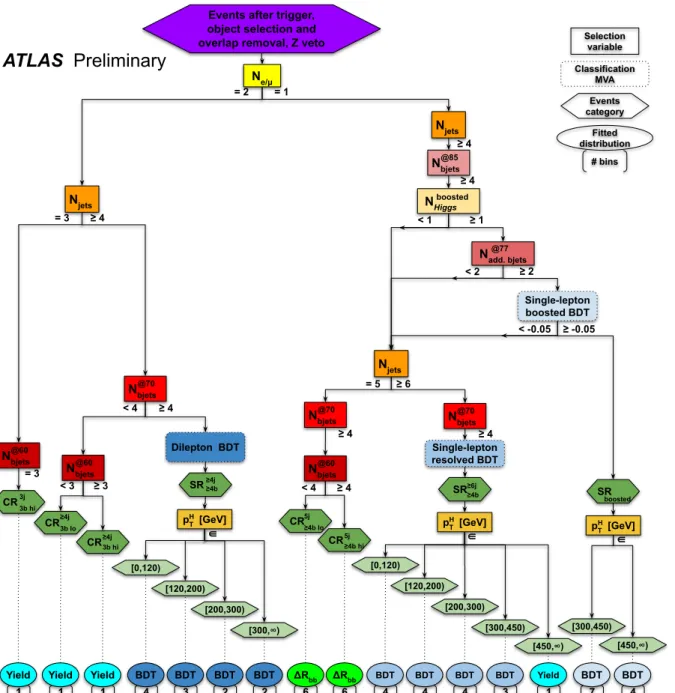
In order to target the t¯ tH(b b) ¯ final state, events are categorised into orthogonal regions defined by the number of leptons, the number of jets, the number of b -tagged jets at different b -tagging efficiencies (60%, 70%, 77%, or 85%) and the number of boosted Higgs boson candidates.

The analysis regions with higher signal-to-background ratio are referred to as ‘signal regions’ (SR). In these regions, multivariate techniques are used to further separate the t¯ tH signal from the background

5

The rapidity is defined as y =

ln

z

where E is the energy and p

is the longitudinal component of the momentum along

the beam pipe.

events. The remaining analysis regions, depleted in signal, are referred to as ‘control regions’ (CR), which provide stringent constraints on the normalisation of the backgrounds and systematic uncertainties in a combined fit with the signal regions.

In the single-lepton channel, events are classified in the boosted category if they contain at least four jets (at least four of which are b -tagged at the 85% working point), one boosted Higgs boson candidate, and at least two jets not belonging to the boosted Higgs boson candidate which are b -tagged at the 77% working point. The boosted Higgs boson candidate must satisfy p

> 300 GeV, have an invariant mass in the range 100–140 GeV, a DNN score P(H) > 0 . 6, and exactly two jet constituents b -tagged at the 85% working point. This selected RC jet is used to determine the kinematic properties of the boosted Higgs boson candidate (reconstructed p

T

, m

, etc.). All other selected events belong to the resolved categories.

The dilepton and single-lepton resolved signal regions are further split according to the reconstructed p

T

(see below) to allow the extraction of multiple signal parameters, sensitive to new physics effects, in five reconstructed p

T

regions: 0–120 GeV, 120–200 GeV, 200–300 GeV, 300–450 GeV and ≥ 450 GeV. The two highest reconstructed p

T

bins are merged in the dilepton case due to an insufficient expected number of events. The boosted signal region, SR

, is split into two reconstructed p

T

regions: 300–450 GeV and ≥ 450 GeV. These ranges are the same as used to define STXS bins with truth p

T

, where the truth p

T

is taken from the MC event record before the Higgs boson decays, and were chosen to minimise the correlation among signal strengths in different STXS bins. Control regions are inclusive in reconstructed p

T

to keep the constraining power on the background composition.

Table 2 defines the 16 regions in which the events are classified: 11 SRs (dilepton SR

, single-lepton SR

and SR

, split according to reconstructed p

T

in four, five and two regions, respectively), and five CRs. After these selections are applied, t¯ t + heavy-flavour jets dominate the background composition and the t¯ tH signal selection efficiency is 1.2%. In the SRs the shape and normalisation of a multivariate discriminant is used in the statistical analysis, except in the highest reconstructed p

T

bin of the single-lepton resolved analysis, where only the event yield is used. In the dilepton CRs only the event yield is used, to correct the amount of t t ¯ + ≥ 1 c predicted from the inclusive t t ¯ + jets sample. In the single-lepton channel the shape and normalisation of the average ∆R for all possible combinations of b -tagged jet pairs, ∆R

, is used in the CRs to help better constrain the background contributions and correct their shape. This variable is one of the inputs to the classification BDT which shows good discriminating power between signal and background. Control regions have different ratios of t¯ t + ≥ 1 b to t¯ t + ≥ 1 c events: regions defined as hi are enriched in t t ¯ + ≥ 1 b while in regions defined as lo the proportion of t t ¯ + ≥ 1 c events is increased. The different proportions of t¯ t + ≥ 1 b and t t ¯ + ≥ 1 c in the control regions allow the signal extraction fit to better constrain the relative fractions of these processes in the signal regions.

Multivariate classifiers are used in two parts of this analysis: identifying Higgs boson candidate objects and classifying t tH ¯ signal events. In all SRs of the resolved categories, the multivariate classifiers are constructed analogously to the reconstruction and classification boosted decision trees (BDTs) used in the previous analysis [26] and trained with TMVA [98] with the same input variables and training parameters.

The training for the reconstruction BDTs is identical to this previous analysis, matching reconstructed jets to the partons emitted from top-quark and Higgs-boson decays. For this purpose, W -boson, top-quark and Higgs-boson candidates are built from combinations of jets and leptons. The b -tagging information is used to discard combinations containing jet–parton assignments inconsistent with the correct parton candidate flavour. The combination of jets with the highest reconstruction BDT score is selected, allowing the computation of kinematic properties of the Higgs boson candidate (reconstructed p

T

, m

, etc.).

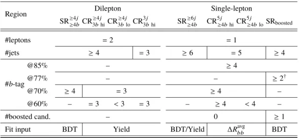
Table 2: Definition of the analysis regions, split according to the number of leptons, jets, and b -tagged jets using different working points, and the number of boosted Higgs candidates. For SR

, b -tagged jets flagged with

are extra b -jets not part of the boosted Higgs boson candidate. All SRs are further split in reconstructed p

T

as described in the text. The last row specifies the type of input to the fit used in each region: normalisation only (Yield) or shape and normalisation of the classification BDT or ∆R

distribution. In the highest p

T

≥ 450 GeV bin of the single-lepton resolved analysis, only the event yield is used.

Region Dilepton Single-lepton

SR

CR

CR

CR

SR

CR

CR

SR

#leptons = 2 = 1

#jets ≥ 4 = 3 ≥ 6 = 5 ≥ 4

# b -tag

@85% – ≥ 4

@77% – – ≥ 2

@70% ≥ 4 = 3 ≥ 4 –

@60% – = 3 < 3 = 3 – ≥ 4 < 4 –

#boosted cand. – 0 ≥ 1

Fit input BDT Yield BDT/Yield ∆R

BDT

The classification BDTs have been trained using the signal and components of the nominal background model presented in this note. The dilepton BDT is trained only against t t ¯ + b b ¯ events (as it constitutes most of the background), the single-lepton resolved BDT is trained against t t ¯ + jets events (because t t ¯ + ≥ 1 c and t t ¯ + light events also contribute) and the single-lepton boosted BDT is trained against all background processes. These BDTs are built by combining kinematic variables, such as invariant masses and angular separations of pairs of reconstructed jets and leptons, outputs of the reconstruction discriminants, as well as the pseudo-continuous b -tagging discriminant of selected jets. The reconstruction discriminants provide their own output value as well as variables derived from the selected combination of jets with the highest reconstruction BDT score in the resolved channels. In the single-lepton resolved channel, a likelihood discriminant method that combines the signal and background probabilities of all possible jet combinations in each event is also used as input to the classification BDT [26]. Distributions of the output of these BDT classifiers serve as SR inputs to the signal extraction fit.

6 Systematic uncertainties

Many sources of systematic uncertainties affect this analysis. Both the shape and normalisation of

distributions can be affected by uncertainties which impact the categorisation of events and the final

discriminants used in the signal extraction fit. All sources of experimental uncertainty considered, with the

exception of the uncertainty in the luminosity, affect both the normalisations and shapes of distributions in

all the simulated samples. Uncertainties related to modelling of the signal and the background processes

affect both the normalisations and shapes of the distributions, with the exception of cross-section and

normalisation uncertainties which only affect the normalisation of the considered sample. Nonetheless,

the normalisation uncertainties modify the relative fractions of the different samples leading to a shape

uncertainty in the distribution of the final discriminant for the total prediction in the different analysis regions.

A single independent nuisance parameter is assigned to each source of systematic uncertainty. Some of the systematic uncertainties, in particular most of the experimental uncertainties, are decomposed into several independent sources, as specified in the following. Each individual source then has a correlated effect across all the channels, analysis regions, signal and background samples. Modelling uncertainties are typically broken down into components which target specific physics effects in the MC calculation, such as additional radiation from scale variations or changing the hadronisation model, and are uncorrelated between different samples.

6.1 Experimental uncertainties

The uncertainty in the combined 2015–2018 integrated luminosity is 1.7% [99], obtained using the LUCID-2 detector [100] for the primary luminosity measurement. An uncertainty associated with the modelling of pileup in the simulation is included to cover the difference between the predicted and measured inelastic cross-section values [101].

The jet energy scale uncertainty is derived by combining information from test-beam data, LHC collision data and simulation, and the jet energy resolution uncertainty is obtained by combining dijet balance measurements and simulation [86]. Additional considerations related to jet flavour, pileup corrections, η dependence and high- p

jets are included. These uncertainties are further propagated into the single-lepton boosted analysis by applying the reclustering described in Section 4 with systematically varied inputs.

A total of 40 independent contributions are considered. While the uncertainties are not large, varying between 1% and 5% per jet (depending on the jet p

), the effects are amplified by the large number of jets considered in the final state. The efficiency to identify and remove jets from pileup is measured with Z → µ

µ

events in data using techniques similar to those used in Ref. [87]. An uncertainty is considered to account for the difference in performance in data and simulation.

The efficiency to correctly tag b -jets is measured using dileptonic t t ¯ events [88]. The mis-tag rate for c -jets is measured using single-lepton t t ¯ events, exploiting the c -jets from the hadronic W -boson decays using techniques similar to Ref. [89]. The mis-tag rate for light-jets is measured using the negative-tag method similar to Ref. [90] applied to Z + jets events. The uncertainty in tagging b -jets is 2%–10% depending on the working point and jet p

. The uncertainty in mis-tagging c -jets is 10%–25% and light-jets is 15%–50% depending on the working point and jet p

. For the calibration of the four working points used in this analysis, a large number of uncertainty components are considered, and a principal component analysis is performed, yielding 45, 20, and 20 uncorrelated sources of uncertainties for b -, c - and light-jets, respectively.

Uncertainties associated with leptons arise from the trigger, reconstruction, identification, and isolation, as well as the lepton momentum scale and resolution. Efficiencies are measured using leptons in Z → `

`

events [83, 84], while scale and resolution calibrations are performed using leptons in Z → `

`

and J/ψ → `

`

events [83, 84]. Systematic uncertainties in these measurements account for 22 independent sources but only have a small impact on the final result.

All uncertainties related to energy scales or resolution of the reconstructed objects are propagated to the

calculation of the missing transverse momentum. Three additional uncertainties associated to the scale and

resolution of the soft term are also included. As the missing transverse momentum is only used for event reconstruction and not for event selection, these uncertainties have a minimal impact.

6.2 Modelling uncertainties

Uncertainties on the predicted SM t tH ¯ signal cross-section are evaluated with a particular focus on the impact on STXS bins. An uncertainty of ± 3 . 6% from varying the PDF and α

in the fixed-order calculation is applied [19, 102–106]. The effect of PDF variations on the shape of the distributions considered in this analysis is found to be negligible. Uncertainties in the Higgs boson branching fractions are also considered, which amount to 2.2% for the b b ¯ decay mode [19]. An uncertainty related to the amount of initial state radiation (ISR) is estimated by simultaneously varying the renormalisation and factorisation scales in the ME and α

in the PS [107], while an uncertainty related to the final state radiation (FSR) is estimated by varying α

in the PS. The nominal PowhegBox+Pythia8 sample is also compared to the PowhegBox+Herwig7 sample to assess an uncertainty related to the choice of PS and hadronisation, and to the MadGraph5_aMC@NLO+Pythia8 sample to assess an uncertainty arising from changing the NLO matching procedure (sample details are given in Table 1). Uncertainties due to missing higher order terms in the perturbative QCD calculations affecting the total cross-section and event migration between STXS bins are estimated by varying the renormalisation and factorisation scales independently by a factor of two, as well as evaluating the ISR and FSR uncertainties. The largest effect was found to originate from the ISR uncertainty, corresponding to a variation of the total cross-section of 9.2%, leading to an uncertainty in the range of 10%–17% on bin migrations estimated using the Stewart-Tackmann procedure [108]. All signal uncertainties are correlated across STXS bins, with the exception of bin migration uncertainties.

The systematic uncertainties affecting the t¯ t + jets background modelling are summarised in Table 3. An uncertainty of 6% is assumed for the inclusive t¯ t production cross-section predicted at NNLO+NNLL, including effects from varying the factorisation and renormalisation scales, the PDFs, α

, and the top-quark mass [45–51]. This uncertainty is applied to t t ¯ + light samples only, since this component is dominant in t¯ t production in the full phase-space. An uncertainty of 100% in the normalisation of t¯ t + ≥ 1 c events is applied, motivated by the fitted value of this normalisation in the previous analysis [26]. The normalisation of t t ¯ + ≥ 1 b is allowed to float freely in the signal extraction fit. The t t ¯ + ≥ 1 b , t¯ t + ≥ 1 c and t t ¯ + light processes are affected by different types of uncertainties: t¯ t + light profits from relatively precise measurements in data; t t ¯ + ≥ 1 b and t t ¯ + ≥ 1 c can have similar or different diagrams depending on the precision of the ME and the flavour scheme used for the PDF, and the different masses of the c - and b -quarks contribute to additional differences between these two processes. For these reasons, all uncertainties in the t¯ t + jets background modelling are assigned independent nuisance parameters for the t t ¯ + ≥ 1 b , t t ¯ + ≥ 1 c and t¯ t + light processes.

Systematic uncertainties in the acceptance and shapes are extracted from the comparison between the

nominal prediction and different MC samples or settings. The fraction of t t ¯ + ≥ 1 b events in the selected

phase-space in all alternative samples is reweighted to match the fraction in the nominal sample. This

is to allow the normalisation of t¯ t + ≥ 1 b to be solely driven by the free-floating parameter in the signal

extraction fit to data. The systematic uncertainties related to varying the amount of ISR, the amount of FSR,

the PS and hadronisation, and the NLO matching procedure are estimated using the same procedure as for

t¯ tH , comparing the nominal prediction to alternative samples. In the specific case of t¯ t + ≥ 1 b , relative

uncertainties are used to estimate the effect of changing the PS and hadronisation or the NLO matching

procedure by comparing predictions from the NLO t¯ t generators (see Table 3). Whilst this comparison

is made using predictions in which the additional b -quarks are generated at a leading-log precision from

gluon splitting, the size of this difference was observed to be generally the same as or larger than the

difference between two different t¯ t + b b ¯ NLO predictions for the distributions entering into the signal extraction fit. The impact of these uncertainties on the final results is reported in Section 7.

Special consideration is given to the correlation of modelling uncertainties across different p

T

bins, in order to provide the fit with enough flexibility to cover background mismodelling without biasing the signal extraction. The NLO matching t t ¯ + ≥ 1 b uncertainty is shown to depend on p

T

and therefore decorrelated across p

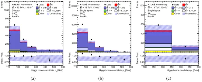
bins in the SRs. The NLO matching and the PS and hadronisation t¯ t + ≥ 1 b uncertainties are further decorrelated between the single-lepton and dilepton channels. The pre-fit distributions of the reconstructed p

T

are shown in Figure 1. An additional uncertainty is derived for the t¯ t + ≥ 1 b sample to cover the mismodelling observed in this distribution. After removing the overall normalisation difference by scaling the t t ¯ + ≥ 1 b background in the dilepton SR

(single-lepton SR

), a weight is computed in each reconstructed p

T

bin of the dilepton SR

(single-lepton SR

), which corrects the predicted t¯ t + ≥ 1 b contribution so that the data and MC yields agree. The derived weights are applied as an additional uncertainty on the t¯ t + ≥ 1 b normalisation in each reconstructed p

T

bin. The weights derived in the single-lepton resolved channel are also applied in the boosted channel. This uncertainty enters the signal extraction fit as a single nuisance parameter ( p

T

shape), correlated across all channels, such that a pull of +1 σ corresponds to applying this weight.

0 100 200 300 400 500 600

[GeV]

Higgs boson candidate pT

0.5 0.75 1 1.25

Data / Pred.

0 200 400 600 800 1000 1200

Events

ATLAS Preliminary = 13 TeV, 139 fb-1

s Dilepton

≥4j

≥4b

SR Pre-Fit

Data ttH

≥1b + t

t tt + ≥1c + V t

t tt + li.,4t,tH Other Uncertainty

(a)

0 100 200 300 400 500 600

[GeV]

Higgs boson candidate pT

0.5 0.75 1 1.25

Data / Pred.

0 2000 4000 6000 8000 10000

Events

ATLAS Preliminary = 13 TeV, 139 fb-1

s Single lepton

≥4b

≥6j

SR Pre-Fit

Data ttH

≥1b + t

t tt + ≥1c + V t

t tt + li.,4t,tH Other Uncertainty

(b)

300 350 400 450 500 550 600

[GeV]

Higgs boson candidate pT

0.5 0.75 1 1.25

Data / Pred.

0 200 400 600 800 Events1000

ATLAS Preliminary = 13 TeV, 139 fb-1

s Single lepton

boosted

SR Pre-Fit

Data ttH

≥1b + t

t tt + ≥1c + V t

t tt + li.,4t,tH Other Uncertainty

(c)

Figure 1: Pre-fit distributions of the reconstructed Higgs boson candidate p

for the (a) dilepton SR

, (b) single-lepton resolved SR

and (c) single-lepton boosted SR

signal regions. The uncertainty band includes all uncertainties and their correlations, except for the uncertainty on the k(t t ¯ + ≥ 1 b) normalisation factor which is not defined pre-fit.

To account for variations in the t t ¯ + ≥ 1 b subcomponent fractions found in different predictions, an additional nuisance parameter is introduced which covers the largest discrepancy between two models for the fraction of t t ¯ + 1 b/ 1 B and t¯ t + ≥ 2 b . The one-sigma variation of this nuisance parameter corresponds to reducing the amount of t¯ t + ≥ 2 b by 19.5% and increasing the amount of t¯ t + 1 b/ 1 B by 41.5%. This uncertainty is correlated across all regions, and impacts each region differently due to the varying compositions of t¯ t + ≥ 1 b .

An uncertainty of 5% is considered for the cross-sections of the three single-top production modes [54, 55, 109, 110]. Uncertainties associated with the PS and hadronisation model, and with the NLO matching

scheme are evaluated by comparing, for each process, the nominal PowhegBox+Pythia8 sample to a

sample produced using PowhegBox+Herwig7 and MadGraph5_aMC@NLO+Pythia8. The uncertainty

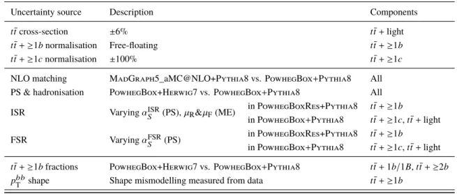
Table 3: Summary of the sources of systematic uncertainty for t t ¯ + jets modelling. The systematic uncertainties listed in the second section of the table are evaluated in such a way as to have no impact on the normalisation of the three t t ¯ + ≥ 1 b , t t ¯ + ≥ 1 c , and t t ¯ + light components in the phase-space selected in this analysis. The last column of the table indicates the t t ¯ + jets components to which a systematic uncertainty is assigned. All systematic uncertainty sources are treated as uncorrelated across the three components.

Uncertainty source Description Components

t¯ t cross-section ± 6% t t ¯ + light

t¯ t + ≥ 1 b normalisation Free-floating t t ¯ + ≥ 1 b

t¯ t + ≥ 1 c normalisation ± 100% t t ¯ + ≥ 1 c

NLO matching MadGraph5_aMC@NLO+Pythia8 vs. PowhegBox+Pythia8 All PS & hadronisation PowhegBox+Herwig7 vs. PowhegBox+Pythia8 All ISR Varying α

(PS), µ

& µ

(ME) in PowhegBoxRes+Pythia8 t t ¯ + ≥ 1 b

in PowhegBox+Pythia8 t t ¯ + ≥ 1 c , t¯ t + light FSR Varying α

(PS) in PowhegBoxRes+Pythia8 t t ¯ + ≥ 1 b

in PowhegBox+Pythia8 t t ¯ + ≥ 1 c , t¯ t + light t¯ t + ≥ 1b fractions PowhegBox+Herwig7 vs. PowhegBox+Pythia8 t t ¯ + 1b / 1B, t¯ t + ≥ 2b p

T

shape Shape mismodelling measured from data t t ¯ + ≥ 1 b

associated to the interference between tW and t t ¯ production at NLO [43] is assessed by comparing the nominal PowhegBox+Pythia8 sample produced using the diagram removal scheme with an alternative sample produced with the same generator but using the diagram subtraction scheme.

An uncertainty of 40% is assumed for the W + jets cross-section, with an additional 30% normalisation uncertainty used for W + heavy-flavour jets, taken as uncorrelated between events with two and more than two heavy-flavour jets. These uncertainties are based on variations of the factorisation and renormalisation scales and of the Sherpa matching parameters. An uncertainty of 35% is applied to the Z + jets normalisation, uncorrelated across jet bins, to account for both the variations of the scales and the Sherpa matching parameters, and the uncertainty in the extraction from data of the correction factor for the heavy-flavour component.

The uncertainty in the t tV ¯ NLO cross-section prediction is 15% [111], split into PDF and scale uncertainties as for t¯ tH . An additional t¯ tV modelling uncertainty, related to the choice of PS and hadronisation model and NLO matching scheme is assessed by comparing the nominal MadGraph5_aMC@NLO+Pythia8 samples with alternative ones generated with Sherpa.

The uncertainty in the diboson background is assumed to be 50%, which includes uncertainties in the

inclusive cross-section and additional jet production [112]. A 50% normalisation uncertainty is considered

for the four-top background, covering effects from varying the factorisation and renormalisation scales,

the PDFs and α

[113]. The small backgrounds from t Z q and tW Z are each assigned cross-section

uncertainties; for t Z q two uncertainties are used, 7.9% accounting for factorisation and renormalisation

scale variations and 0.9% accounting for PDFs, and for tW Z a single uncertainty of 50% is used [113].

7 Results

The distributions of the classification BDT in the signal regions, and the event yield or the ∆R

distributions in the dilepton or single-lepton control regions, respectively, are combined in a profile likelihood fit to extract the signal, while simultaneously determining the yields and constraining the normalisation and shape of differential distributions of the most important background components.

The statistical analysis is based on a binned likelihood function L(µ, θ) constructed as a product of Poisson probability terms over all bins considered in the analysis. The likelihood function depends on the signal-strength parameter µ , defined as µ = σ/σ

(where σ is the measured cross-section and σ

is the Standard Model prediction) and θ , where θ is the set of nuisance parameters which characterise the effects of systematic uncertainties on the signal and background expectations. They are implemented in the likelihood function as Gaussian or Poisson priors, with the exception of the unconstrained normalisation factor k(t¯ t + ≥ 1 b) for the t¯ t + ≥ 1 b background, on which no prior knowledge from theory or subsidiary measurements is assumed. The statistical uncertainty in the prediction, which incorporates the statistical uncertainty deriving from the limited number of simulated events, is included in the likelihood in the form of additional nuisance parameters, one for each of the considered bins. In the statistical analysis, the number of expected events in a given bin depends on µ and θ . The nuisance parameters θ adjust the expectations for signal and background according to the corresponding systematic uncertainties, and their fitted values correspond to the amount that best fits the data. The test statistic t

is defined as the profile likelihood ratio: t

= − 2 ln (L(µ, θ ˆˆ

)/L( µ, ˆ θ)) ˆ , where ˆ µ and ˆ θ are the values of the parameters that maximise the likelihood function and θ ˆˆ

are the values of the nuisance parameters that maximise the likelihood function for a given value of µ [114]. This test statistic is used to measure the compatibility of the observed data with the background-only hypothesis (i.e. for µ = 0), and to make statistical inferences about µ , as implemented in the RooStat framework [115, 116]. The uncertainty in the best-fit value of the signal strength is extracted by finding the values of µ that correspond to varying t

by one unit.

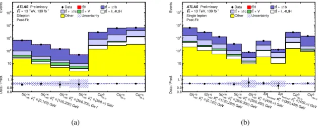
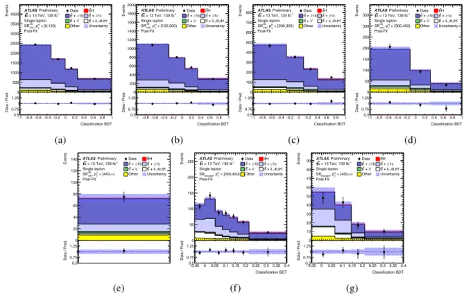
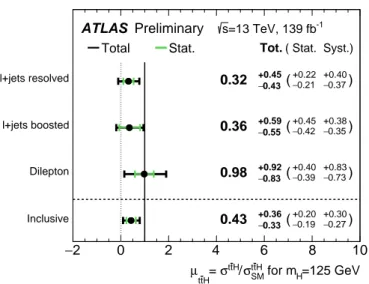
Tables 4 and 5 and Figure 2 show the observed and predicted event yields in all SRs and CRs after the fit to data. The SR BDT distributions are presented in Figures 3 and 4. All distributions are compatible with the data. The normalisation factor for the t¯ t + ≥ 1 b background is found to be k(t¯ t + ≥ 1 b) = 1 . 26 ± 0 . 09. The best-fit µ value is

µ = 0 . 43

(stat.)

(syst.) = 0 . 43

,

corresponding to an observed (expected) significance of 1.3 (3.0) standard deviations with respect to the background-only hypothesis.

The statistical uncertainty is obtained by repeating the fit to data after fixing all nuisance parameters to

their post-fit values, with the exception of the free normalisation factors in the fit: k (t t ¯ + ≥ 1 b) and µ . The

total systematic uncertainty is obtained from the subtraction in quadrature of the statistical uncertainty

from the total uncertainty. The expected significance is computed from a fit to a pseudo-dataset, built using

pulls from the nominal fit when fixing µ = 1. The global goodness of fit, including all input variables to

the classification BDTs and to a fit using the saturated model [117], is 86%, validating the good post-fit

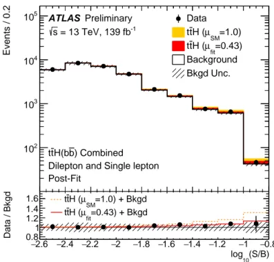
modelling achieved. Figure 5 shows the event yield in data compared to the post-fit prediction for all events

entering the analysis selection, grouped and ordered by the signal-to-background ratio of the corresponding

final-discriminant bins. The measured signal strength is compatible with that obtained previously [26] on

part of the dataset, with systematic uncertainties reduced by a factor of two.

SR

CR

hi

CR

hi

CR

lo

p

T

range [GeV] [0,120) [120,200) [200,300) [300, ∞ )

t¯ tH 14 ± 12 6.7 ± 5.3 3.3 ± 2.6 1.6 ± 1.2 10.5 ± 8.4 51 ± 41 33 ± 27

t¯ t + ≥ 1b 557 ± 28 265 ± 17 117.6 ± 9.6 37.4 ± 5.6 2030 ± 130 4080 ± 210 2540 ± 170 t¯ t + ≥ 1 c 48.7 ± 9.5 14.4 ± 4.4 6.2 ± 1.4 3.9 ± 1.0 523 ± 130 1190 ± 260 2550 ± 500 t¯ t + light, 4 t , tH 7.9 ± 5.8 4.2 ± 2.8 2.1 ± 1.5 1.4 ± 1.3 123 ± 66 221 ± 120 923 ± 360 t¯ t + Z 12.5 ± 2.0 7.6 ± 1.6 4.15 ± 0.71 2.03 ± 0.44 10.7 ± 1.7 57.4 ± 7.3 52.5 ± 6.8 t¯ t + W 0.75 ± 0.31 0.41 ± 0.12 0.27 ± 0.11 0.128 ± 0.069 1.83 ± 0.55 10.9 ± 1.6 22.0 ± 3.5 Other top sources 19.0 ± 6.7 7.7 ± 4.2 4.4 ± 4.0 2.0 ± 1.5 126 ± 34 208 ± 60 254 ± 71 Fakes 3.6 ± 1.1 1.32 ± 0.51 0.40 ± 0.23 0.57 ± 0.30 6.31 ± 1.8 46.3 ± 12 55.7 ± 14 Total 664 ± 24 307 ± 16 138.5 ± 8.9 48.9 ± 5.1 2830 ± 54 5860 ± 79 6430 ± 82

Data 647 306 135 48 2827 5865 6429

Table 4: Post-fit event yields in the dilepton channel signal and control regions. All uncertainties are included, taking into account correlations.

SR^≥6j_≥4b SRboosted CR^5j_≥4blo CR^5j_≥4bhi

p^H

Trange [GeV] [0,120) [120,200) [200,300) [300,450) [450,∞) [300,450) [450,∞)

t¯tH 93±74 49±39 26±21 5.9±4.6 1.26±1.00 15±12 3.6±2.8 26±20 26±21

tt¯+≥1b 4450±160 2040±85 855±43 234±20 43.4±8.2 297±27 51.0±9.8 1595±80 1102±51 t¯t+≥1c 960±210 404±87 179±38 46±11 12.9±3.3 157±37 40±11 630±140 90±23 t¯t+ light, 4t,tH 250±140 105±57 52±26 15.4±8.8 3.5±2.2 62±25 16.9±7.6 270±100 26±16 t¯t+W 7.3±1.1 4.46±0.87 2.54±0.48 1.09±0.31 0.48±0.14 1.89±0.36 0.57±0.17 2.62±0.46 0.53±0.12 t¯t+Z 79±10 46.0±6.4 31.1±4.9 11.8±2.3 2.12±0.64 11.0±2.1 2.34±0.60 25.9±3.5 22.8±3.1 Single topWt 80±43 44±27 18.7±7.8 9.5±9.0 6.1±5.4 14.0±8.3 4.9±4.3 60±32 28±20 Other top sources 48±25 24±16 14±10 4.5±2.7 1.09±0.54 4.4±3.0 0.88±0.78 41±16 28±11 V&VV+ jets 63±24 30±11 20.6±8.2 8.1±3.4 1.92±0.84 13.1±5.6 4.2±2.0 43±15 24.9±8.8 Total 6026±84 2747±52 1198±31 336±15 72.8±7.0 575±23 124.4±9.7 2700±52 1348±38

Data 6047 2742 1199 331 75 581 118 2696 1362

Table 5: Post-fit event yields in the single-lepton resolved and boosted signal and control regions. All uncertainties are included, taking into account correlations.

[0,120) GeV H∈ T 4j, p

≥ 4b

≥ SR

[120,200 H∈ T 4j, p

≥ 4b

≥ SR

[200,300 H∈ T 4j, p

≥ 4b

≥ SR

) GeV [300,∞ H∈ T 4j, p

≥ 4b

≥

SR 3j

3b hi

CR ≥4j

3b hi

CR ≥4j

3b lo 0.8 CR

0.91.11

Data / Pred.

1 10 102 103 104 105

Events

ATLASPreliminary

= 13 TeV, 139 fb-1 s

Dilepton Post-Fit

Data ttH tt+ ≥1b

1c + ≥

tt tt+ V tt+ li.,4t,tH Other Uncertainty

) GeV ) GeV

(a)

[0,120) Ge V H∈ T 4b, p

≥ 6j SR≥

[120,200 H∈ T 4b, p

≥ 6j SR≥

[200,300 H∈ T 4b, p

≥ 6j SR≥

[300,450 H∈ T 4b, p

≥ 6j SR≥

) GeV [450,∞ H∈ T 4b, p

≥ 6j SR≥

H∈ T , p boosted SR

) GeV [450,∞ H∈ T , p boosted SR

4b lo

≥ CR5j

4b hi

≥ CR5j 0.80.91.11

Data / Pred.

1 10 102 103 104 105

Events

ATLASPreliminary

= 13 TeV, 139 fb-1 s

Single lepton Post-Fit

Data ttH tt+ ≥1b

1c + ≥

tt tt+ V tt+ li.,4t,tH Other Uncertainty

[300,450 ) GeV ) GeV

) GeV ) GeV

(b)

Figure 2: Comparison of predicted and observed event yields in each of the control and signal regions in the (a)

dilepton and (b) single-lepton channels after the fit to the data. The uncertainty band includes all uncertainties and

their correlations.