Higgs Boson Production via Vector Boson Fusion in Decays into W Bosons

Dissertation

Measurement of

Higgs Boson Production via Vector Boson Fusion in Decays into W Bosons

with the ATLAS Detector

von

Johanna Bronner

erstellt am

Max-Planck-Institut f¨ ur Physik (Werner-Heisenberg-Institut)

eingereicht an der

Fakult¨at f¨ ur Physik

der

Technischen Universit¨at M¨ unchen

M¨ unchen

M¨arz 2014

Fakult¨at f¨ ur Physik der Technischen Universit¨at M¨ unchen Max-Planck-Institut f¨ ur Physik

(Werner-Heisenberg-Institut)

Measurement of

Higgs Boson Production via Vector Boson Fusion in Decays into W Bosons

with the ATLAS Detector

Johanna Bronner

Vollst¨ andiger Abdruck der von der Fakult¨ at f¨ ur Physik der Technischen Universit¨ at M¨ unchen zur Erlangung des akademischen Grades eines

Doktors der Naturwissenschaften (Dr. rer. nat.) genehmigten Dissertation.

Vorsitzender: Univ.-Prof. Dr. A. Ibarra Pr¨ ufer der Dissertation:

1. Priv.-Doz. Dr. H. Kroha 2. Univ.-Prof. Dr. L. Oberauer

Die Dissertation wurde am 21.03.2014 bei der Technischen Universit¨ at M¨ unchen

eingereicht und durch die Fakult¨ at f¨ ur Physik am 08.04.2014 angenommen.

F¨ur meine Großm¨utter Ingeborg Schoppel

und Elisabeth Bronner

Abstract

The vector boson fusion production rate of the Standard Model Higgs boson has been measured in decays into two W bosons, each subsequently decaying into an electron or muon and a neutrino, with the ATLAS detector at the Large Hadron Collider (LHC). The vector boson fusion production cross section in the Standard Model is about an order of magnitude smaller than the dominant Higgs boson production cross section from gluon fusion.

Proton-proton collision data at a center-of-mass energy of 8 TeV delivered by the LHC recorded with the ATLAS detector corresponding to an integrated luminosity of 21 fb

have been analyzed. Motivated by the recent discovery of a Higgs-like boson with a mass of (125.5

0.6) GeV and (125.7

0.4) GeV by the ATLAS and CMS collaborations at the LHC, the analysis is optimized for this mass. An excess of events, compatible with the Standard Model expec- tation for a Higgs boson with m

= 125 GeV, is observed with a significance of 2.8 standard deviations when compared to the background-only expecta- tion. The corresponding signal strength, the observed event rate relative to the Standard Model prediction of m

= 125 GeV is 2.1

. A Higgs boson produced via vector boson fusion is excluded with 95% confidence level in the mass range between 152 GeV and 185 GeV.

When combined with measurements of other Higgs boson production and

decay channels by ATLAS, evidence for vector boson fusion production with

a significance of 3.3 standard deviations is observed. All measurements of

Higgs boson couplings to Standard Model particles are in agreement with

the predictions of the Standard Model.

Acknowledgments

I would like to thank Sandra Kortner and Hubert Kroha for accepting me as a PhD student and guiding me through the past years. I am in particular thankful for the long term stay at CERN. It has been a unique chance I deeply appreciate. Also I am very thankful for all the time they devoted in the thesis corrections. In addition I would like to thank Robert Richter, Rikard Sandstr¨ om, Max Goblirsch-Kolb and Hans Lehmann for their help.

Many thanks also to Olivier Arneaz, who helped me a lot with all the physics related questions, that came up while writing up the thesis.

I am very thankful for the social and professional environment I worked within. Thanks to all those at CERN and at the MPP for many fruitful physics discussions and pleasant social activities. I would like to thank Eve- lyn Schmidt for opening me the doors to the HSG3 group and Joana Machado Migu´ ens for our very good cooperation. Thanks to Sebastian Stern for his en- chanting travel company and for losing all those bets. Lastly, special Thanks to Philipp Schwegler for being the best possible office mate.

I am very grateful for the support of my family in particular of Anne, Nina and Dorothea Bronner. Thanks to all my friends bearing with the little time I invested in our friendships the past years. I am in particular thankful to the Family Becerici-Schmidt, whose house has become a shelter where all the PhD problems seemed largely irrelevant.

Through all the ups and downs of the past years I have been a generally

cheerful person with a strong believe that everything will be alright, thanks

to Jonathan Burdalo Gil, who pushed me when I needed a push, who made

me relax when I needed to relax and who made me laugh, when life didn’t

give me much reason to. Thank you for making me the happy person I am.

Contents

Abstract iii

Acknowledgments v

Contents vii

1 Introduction 1

2 The Higgs Boson in the Standard Model 3

2.1 The Standard Model of Elementary Particles . . . . 3

2.2 Higgs Boson Production in Proton-Proton Collisions . . . . 9

2.2.1 Phenomenology of Proton-Proton Scattering . . . . 9

2.2.2 Higgs Boson Production at the LHC . . . . 13

2.2.3 Higgs Boson Decays . . . . 16

2.2.4 Event Generation and Simulation . . . . 18

2.3 Higgs Boson Properties . . . . 20

3 The ATLAS Detector at the Large Hadron Collider 23

3.1 The Large Hadron Collider . . . . 23

3.2 The ATLAS Detector . . . . 27

3.2.1 The ATLAS Coordinate System . . . . 28

3.2.2 The Inner Detector . . . . 30

3.2.3 The Calorimeter System . . . . 31

3.2.4 The Muon Spectrometer . . . . 33

3.2.5 The Trigger and Data Acquisition System . . . . 34

3.2.6 Luminosity Measurements . . . . 35

3.2.7 Detector Simulation . . . . 35

CONTENTS

4 Reconstruction of Physics Objects 37

4.1 Track and Vertex Reconstruction . . . . 38

4.1.1 Track Reconstruction . . . . 39

4.1.2 Primary Vertex Reconstruction . . . . 39

4.2 Jet Reconstruction and Energy Calibration . . . . 40

4.2.1 Jet Reconstruction . . . . 40

4.2.2 Jet Energy Calibration . . . . 42

4.3 b-jet Identification . . . . 44

4.4 Electron Reconstruction . . . . 45

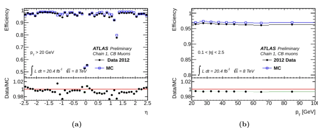
4.5 Muon Reconstruction . . . . 47

4.6 Missing Transverse Energy Reconstruction . . . . 50

4.7 Trigger Requirements . . . . 53

4.7.1 Muon Trigger . . . . 54

4.7.2 Electron Trigger . . . . 55

5 Measurement of the VBF H →`ν`ν Production Rate 57

5.1 Analysis Strategy . . . . 57

5.2 Signal and Background Processes . . . . 58

5.2.1 The Signal Signature . . . . 59

5.2.2 The Background Processes . . . . 61

5.3 The Event Selection . . . . 68

5.4 Background Determination from Data . . . . 78

5.4.1 Measurement of the W +jets and Multijet Background . . . . 81

5.4.2 Measurement of the Z/γ

`` Background . . . . 85

5.4.3 Measurement of the Top Quark Background . . . . 92

5.4.4 Measurement of the Z/γ

τ τ

`ν`ν Background . . . 100

5.4.5 Summary of the Background Measurements . . . 107

5.5 Systematic Uncertainties . . . 109

5.5.1 Theoretical Uncertainties . . . 109

5.5.2 Experimental Uncertainties . . . 113

5.6 Results . . . 115

5.6.1 Comparison of Data and Predictions . . . 115

5.6.2 Statistical Methods . . . 122

5.6.3 The Final Results . . . 129

viii

CONTENTS

5.7 Analysis Improvements . . . 139

5.7.1 Event Categorization in the Signal Region . . . 139

5.7.2 Background Rejection in Same-Flavor Final States . . . 143

6 Combined Analysis of Higgs Production and Decay Channels 147

6.1 The `ν`ν Final State . . . 148

6.2 The Diphoton and Four-Lepton Final State . . . 152

6.3 Measurement of the Signal Production Strengths . . . 157

6.4 Measurement of Coupling Strengths . . . 160

7 Summary 167

Appendices 169

A Monte-Carlo Samples 171

B Background Composition 181

C Top Quark Background Uncertainty 187

D Individual Dilepton Flavor Results 191

Bibliography 195

List of Figures 209

List of Tables 213

Chapter 1

Introduction

The Standard Model, developed in the second half of the 20th century, successfully describes the interactions between the elementary particles via the principle of local gauge symmetry. Its predictions have been precisely confirmed by experiments. No contradictions to the Standard Model have yet been observed. In particular, the Standard Model explains the masses of the gauge bosons mediating the weak interaction and the origin of fermion masses by the Higgs mechanism developed by Englert, Brout [1] and Higgs [2,3] as well as Hagen, Guralnik and Kibbel [4]. The mechanism predicts a massive scalar particle, the Higgs boson, which couples to all massive Standard Model particles.

A description of the Standard Model and the Higgs mechanism as well as a summary of the predictions of the Higgs boson properties is given in Chapter 2.

The discovery of the Higgs boson is an essential step in verifying the Higgs mechanism.

The Large Hadron Collider (LHC) at CERN, designed for colliding proton beams with a center-of-mass energy of 14 TeV, has been constructed in order to finally discover the Higgs boson. It is in operation since autumn 2009 with an interruption for repairs in 2013 and 2014. The beam energies reached 4 TeV in 2012. Data corresponding to an integrated luminosity of 21 fb

were collected at this energy. Another 5 fb

of data were collected at a center-of-mass energy of 7 TeV in 2011. The design energy is expected to be reached with the restart of the LHC in 2015.

The data used in this thesis have been recorded with the ATLAS

detector at the LHC. The detector is described together with the LHC accelerator system in Chapter 3.

The reconstruction of particles and jets, physics objects needed for the analysis, is described in Chapter 4.

∗ATLAS: A Toroidal LHC AparatuS

Chapter 1. Introduction

In July 2012 the ATLAS [5] and CMS

[6] experiments discovered a Higgs boson candidate. Employing the full available dataset a mass of 125.5 GeV [7] and 125.7 GeV [8]

was measured by the ATLAS and CMS experiments, respectively. The properties of the boson have been tested in detail for their compatibility with the Standard Model predictions. One necessary test is the verification of the different production and decay processes predicted by the Standard Model.

The thesis focusses on the measurement of the production of the Higgs boson through Vector Boson Fusion (VBF) in the decay channel into two W bosons, each subsequently decaying into an electron or muon accompanied by a neutrino, i.e. H

W W

`ν`ν.

This final state is one of the most important Higgs boson search channels due to the large branching fraction and clear signature. The VBF production mode is identified by its characteristic signature with two energetic jets in the final state produced dominantly in forward direction and well separated in rapidity.

Different processes contribute to the background of this channel. The largest ones are W boson and top-quark-pair production as well as Drell-Yan processes. The gluon fusion production of the Higgs boson with an order of magnitude larger cross section than the VBF production counts as a background contribution. The background expectation from Monte-Carlo simulations are, wherever possible, corrected for using control measurements.

The event selection, background determinations and results for this analysis are presented in Chapter 5.

Finally, the combination of the above result with other Higgs boson decay channels in VBF and gluon fusion preselection measurements by the ATLAS experiment are presented in Chapter 6. The result of a combined VBF production rate measurement as well as the measurement of the Higgs boson couplings to Standard Model particles are discussed.

∗CMS: Compact Muon Solenoid

2

Chapter 2

The Higgs Boson

in the Standard Model

This chapter introduces the theoretical framework for this thesis. It begins with an introduction to the

of particle physics in Section 2.1 (see also [9]).

In Section 2.2 the theoretical predictions for Higgs boson production cross sections at hadron colliders and the Higgs boson decay branching ratios are discussed. The discovery of the Higgs boson candidate and the results of its property measurements with the ATLAS and CMS experiments at the LHC are outlined in Section 2.3.

Throughout this thesis natural units are used, with

= c = 1, such that momentum and mass have units of energy.

2.1 The Standard Model of Elementary Particles

The Standard Model is a quantum field theory based on local gauge symmetries with the symmetry group

SU (3)

SU (2)

U (1) , (2.1)

comprising the color symmetry SU (3) of the strong interaction and the symmetry SU (2)

U (1) of the electroweak interaction

. The latter is spontaneously broken by the

structure of the gauge symmetry. Since the gauge theories are renormalizable precise predictions in higher-order perturbation theory are possible (see Section 2.2). The Standard Model has been verified in many experimental tests. Up to now no significant

∗The gravitational force is not included in the Standard Model.

Chapter 2. The Higgs Boson in the Standard Model deviations from the Standard Model have been found.

All particles described by the Standard Model have been observed, including a Higgs boson candidate. The elementary particles of the Standard Model (see Table 2.1) are classified in the following way:

Fermions:

Two types of fermions, both with spin-1/2, are the building blocks of matter:

quarks

and

While quarks participate in all known interactions, leptons do not interact strongly and neutrinos in addition do not interact electromagnetically. Three generations of quarks and leptons have been observed. The masses of the fermions spread over a large range. For each fermion f an anti-fermion ¯ f with the same mass and opposite electric charge and parity quantum number exists.

Vector Bosons

carrying spin-one are the mediators of the fundamental interactions:

Eight gluons for the strong, W

and Z

bosons for the weak and the photon for the electromagnetic interaction. The W

and Z

bosons are massive while the gluons and the photon are massless.

Higgs Boson:

The only elementary spin-zero particle described by the Standard Model is the scalar (CP even) Higgs boson. It is predicted to be massive.

The fundamental interactions of the particles in the Standard Model are described by local quantum gauge field theories with the simplest unitary symmetry groups U (1), SU (2) and SU (3):

• Quantum electrodynamics (QED)

[12–17] describes the electromagnetic in- teraction between electrically charged particles which is mediated by the massless photon and defined by the Abelian U (1) gauge symmetry.

•

The

is described together with the electromagentic interaction by the Glashow-Salam-Weinberg theory [18–21], a non-Abelian SU (2)

U (1) gauge theory. It is mediated by the massive W

, W

and Z

bosons.

• Quantum chromodynamics (QCD)

[22] describes the strong interaction be- tween particles carrying color charge and is defined by the non-Abelian SU (3) gauge symmetry. Eight massless gluons carrying different combinations of color and anti-color are the mediators of the strong interaction. A characteristic of QCD

4

2.1 - The Standard Model of Elementary Particles

Table 2.1: Overview of the particles in the Standard Model. J denotes the spin and P the parity of the particle. The masses are taken from [7, 10, 11]. The uncertainties for the lepton masses are below 0.01%.

Name Symbol Charge[e] Mass

Fermions Leptons

J

= 1 / 2

Electron neutrino ν

0 < 2 eV

Electron e -1 0.511 MeV

Myon neutrino ν

0 < 0.12 MeV

Myon µ -1 105.7 MeV

Tau neutrino ν

0 < 18.2 MeV

Tau τ -1 1.777 GeV

Quarks

J

= 1 / 2

Up u +2/3 2.3

MeV

Down d

1/3 4.8

MeV

Strange s +2/3 95

5 MeV

Charm c

1/3 1.275

0.025 GeV

Bottom b +2/3 4.18

0.03 GeV

Top t

1/3 173.29

0.95 GeV

Bosons Vector

J

= 1

Gluon g 0 0

Photon γ 0 0

W boson W

1 80.385

0.015 GeV

Z boson Z

0 91.1876

0.0021 GeV

Scalar

J

= 0

Higgs boson H 0 125.6

GeV

Chapter 2. The Higgs Boson in the Standard Model

is that the strong coupling constant α

increases with distance. Particles carrying color charges, gluons and quarks, are

in color-singlet bound states of either quark-antiquark pairs (mesons) or triplets of quarks (baryons). At short distances, the strong coupling strength decreases and quarks and gluons behave like free particles inside the bound states (asymptotic freedom).

Non-Abelian gauge symmetries, as for QCD and the weak interaction, lead to self interaction of the mediating vector bosons which is not present for the photon. Local gauge theories predict massless gauge bosons mediating the interactions, like the photon and the gluons. This is in contradiction with the observed large masses of the weak gauge bosons W

and Z

. The theory of the electroweak interaction unifying the electromagnetic and weak forces provides a mechanism to overcome this problem.

Electroweak Unification

The electroweak interaction is a unification of the elec- tromagnetic and weak forces with the gauge symmetry SU (2)

U (1) introduced by Glashow [18], Salam [20, 21] and Weinberg [19]. The SU (2) and U (1) gauge symmetries require four massless vector fields. The vector fields corresponding to the SU (2) group are denoted by W

(a = 1, 2, 3) and the vector field of the U (1) group by B

. The observed W

and Z

boson fields and the photon field A

are related to the four vector fields W

and B

by the transformation

W

= 1

√

2 (W

iW

) ,

Z

= W

cos θ

B

sin θ

, A

= W

sin θ

+ B

cos θ

(2.2)

where the rotation angle θ

is the

e and the gauge coupling strengths g and g

corresponding to the SU (2) and U (1) groups, respectively, by

e = g

sin θ

= g

cos θ

. (2.3)

The electroweak gauge symmetry SU (2)

U (1) is sponta- neously broken to the U (1) symmetry of the electromagnetic interaction,

SU (2)

U(1)

−−−−−−−−−−−−→

symmetry breaking

U (1) , (2.4)

6

2.1 - The Standard Model of Elementary Particles

2) Φ

1, Φ V(

Φ1

Φ2

= v/2 λ

2/2 µ r = -

Figure 2.1: Illustration of the shape of the Higgs potential V depending on the real and imaginary parts Φ1 and Φ2of a complex scalar field breaking localU(1) symmetry. The minima of the potential lie on a circle with radiusr=p

Φ²₁+ Φ²₂=v/2 around the origin.

giving masses to the weak gauge bosons W

and Z

while the photon corresponding to the remaining unbroken U (1) symmetry of QED stays massless. This mechanism, the

well as Guralnik, Hagen and Kibble [4].

In its minimal version, the Higgs-mechanism of the Standard Model introduces a SU (2) doublet of complex scalar fields

Φ = φ

φ

!

. (2.5)

The self-interaction potential of this scaler Higgs doublet field,

V (Φ) = µ

Φ

Φ + λ(Φ

Φ)

, (2.6) has, for λ > 0 and µ

< 0, a shape as illustrated in Fig. 2.1 in the example of U (1) symmetry breaking. The potential has a minimum fulfilling the criterion

Φ

Φ =

µ

2λ

v

2 , (2.7)

where v is called the vacuum expectation value of the scalar field. While the full set

Chapter 2. The Higgs Boson in the Standard Model

of ground states is SU (2)

U (1) symmetric, choosing one specific ground state or vacuum spontaneously breaks the symmetry leaving only a U (1) symmetry for the electromagnetic interaction. A possible choice of ground state is

Φ

= 1

√

2 0 v

!

. (2.8)

Excitations from the ground state can be parameterized by:

Φ(x) = exp[iT

θ

(x)]

√

2

0 v + H(x)

!

(2.9) where θ

are three scalar fields corresponding to massless Goldstone bosons which accompany the symmetry breaking [23, 24]. The Goldstone bosons correspond to excita- tions within the set of symmetric ground states, i.e. tangential to the circle of minima in the example in Fig. 2.1. The Goldstone fields can be eliminated by a local gauge transformation (unitary gauge)

Φ(x)

Φ

(x) exp[

iT

θ

(x)] . (2.10) The additional scalar field H(x), a massive excitation, i.e. orthogonal to the set of ground states, cannot be transformed away. H(x) is called the

field.

The W

and Z

boson acquire masses by absorbing the degrees of freedom of the three Goldstone bosons after the gauge transformation, while the photon field A

remains massless. The masses of the weak gauge bosons are given by

m

= vg

2 = m

cos θ

, (2.11)

in lowest order of perturbation theory. The Higgs boson mechanism also leads to cou- plings between the Higgs boson H and the weak vector bosons V = W, Z with a strength given by

g

=

2i m

v and g

=

2i m

v

. (2.12)

Since the masses of the W

and Z

bosons are related via the weak mixing angle θ

(Eq. (2.11)), the strengths of the Higgs boson coupling to the W

and Z

are related as well which is referred to as

8

2.2 - Higgs Boson Production in Proton-Proton Collisions Fermions acquire their masses by

to the scalar field with a strength of g

proportional to the fermion masses m

not predicted by the Standard Model:

g

= im

√

2

v . (2.13)

The mass m

=

2λv

of the Higgs boson, is also not predicted by the Standard Model like the Higgs self interaction strength λ. However, since λ > 0 is required for spontaneous symmetry breaking, the Higgs boson cannot be massless. The existence of a massive scalar particle, like the Higgs boson is needed to preserve, for instance, unitarity in W W scattering.

2.2 Higgs Boson Production in Proton-Proton Collisions

In this section the theoretical predictions for Higgs boson production and decays at proton colliders are outlined (see [25]). The calculation of production cross sections at proton colliders has to take into account that protons are composite particles. The processes of interest take place between proton constituents and are accompanied by interactions of the residual constituents. These calculations are explained in Section 2.2.1.

A more detailed summary can be found in [26].

The main mechanisms of Higgs boson productions are discussed in Section 2.2.2.

The most important Higgs boson decays are discussed in Section 2.2.3. The predicted differential cross sections and decay rates for signal and background processes are used in Monte-Carlo generators to simulate events that can be compared to real collision data. The event generators used are described in Section 2.2.4.

2.2.1 Phenomenology of Proton-Proton Scattering

Protons are composite particles, consisting of three valence quarks, gluons and sea

quarks, together called partons. A parton-parton collisions is classified as either hard

or soft depending on the momentum transfer in the collision. QCD calculations are

much more precise for hard than for soft processes, since for large momentum transfer

perturbation theory is applicable. The soft processes however, are by far dominating at

hadron colliders. A hard scattering process is, therefore, usually accompanied by soft

reactions taking place between the partons not participating in the hard scatter process.

Chapter 2. The Higgs Boson in the Standard Model

f

A

ˆ σ

f

B

UE

X(HS)

X(HS)

a b

Figure 2.2: Factorization of proton-proton scattering into the hard scattering (HS) process ab →X with cross section ˆσ_ab→X and the remaining soft scattering processes leading to the underlying event (UE). The functionsf_a/Aandf_b/B are the experimentally determined Parton Distribution Functions (PDF) describing the momentum distribution of quarks and gluons in the proton.

The soft part of a proton-proton collision is referred to as the

To describe the proton-proton interaction of two protons A and B, the process is

into its hard and its soft part (see Fig. 2.2). For the hard reaction ab

X of two partons a and b in the two protons into a final state X pertubation theory can be used to calculate the cross section ˆ σ

. The total proton scattering cross section σ

can then be determined as:

σ

=

dx

dx

f

(x

, µ

) f

(x

, µ

) ˆ σ

. (2.14) The function f

(x

) is the

(PDF), which depends on the parton momentum fraction x

= p

/E

.

Perturbative QCD corrections, in particular from collinear gluon radiation from the incoming quarks, leads to large logarithmic terms. Factorization theorems [27] tell that the logarithmic terms for the hard scattering processes can be absorbed in the PDF introducing a dependence on the

µ

which can be understood as the energy scale separating hard and soft physics.

The perturbative calculation of the hard scattering processes leads to expressions in powers of the strong coupling constant α

depending on the renormalization scale µ

relevant for the process:

ˆ

σ

= ˆ σ

+ α

(µ

)ˆ σ

+ . . . . (2.15)

10

2.2 - Higgs Boson Production in Proton-Proton Collisions

0.1 1 10

10^-7 10^-6 10^-5 10^-4 10^-3 10^-2 10^-1 10⁰ 10¹ 10² 10³ 10⁴ 10⁵ 10⁶ 10⁷ 10⁸ 10⁹

10^-7 10^-6 10^-5 10^-4 10^-3 10^-2 10^-1 10⁰ 10¹ 10² 10³ 10⁴ 10⁵ 10⁶ 10⁷ 10⁸ 10⁹

σ_jet(E_T^jet > √s/4)

Tevatron LHC

σ_t

σ_Higgs(M_H = 500 GeV) σ_Z σ_jet(E_T^jet > 100 GeV)

σ_Higgs(M_H = 150 GeV) σ_W σ_jet(E_T^jet > √s/20)

σ_b σ_tot

proton - (anti)proton cross sections

σ (nb)

√s (TeV)

events/sec for L = 1033 cm-2 s-1

Figure 2.3: Next-to-leading-order cross sectionsσas well as the expected number of events for an integrated lumniosity ofL= 10³³s⁻¹cm⁻² of Standard Model processes inpp(LHC) and p¯p(Tevatron) collisions as a function of the center-of-mass energy√s(from [26]).

Chapter 2. The Higgs Boson in the Standard Model

Figure 2.4: Inclusive Higgs boson cross section in proton-proton collisions as a function of the Higgs boson mass (from [26]).

Cross sections at hadron colliders calculated up to next-to-leading order in perturbation theory as a function of the center-of-mass energy are shown in Fig. 2.3. Figure 2.4 shows the inclusive Higgs boson cross section as a function of the Higgs boson mass calculated at leading-order (LO), next-to-leading-order (NLO) and next-to-next-to-leading-order (NNLO) in perturbation theory. The higher-order corrections are significant.

The calculated cross sections do not depend on the choice of the two scales µ

and µ

if all terms of the perturbation series are included. However, at finite order, a proper choice for the scales has to be made. A very common choice is µ

= µ

= Q, with the momentum transfer Q of the hard scattering process. The more higher-order terms there are calculated, the smaller the dependence on the scales is expected to be. To account for the residual scale dependence from unknown higher-order terms, a theoretical uncertainty is assigned to the predicted cross sections estimated from variations of µ

and µ

.

While the dependence of the PDFs on µ

can be determined theoretically [28], the dependence on the parton momentum x

is obtained from fitting deep inelastic scattering data. Two PDF determinations, CT10 [29] and CTEQ6L1 [30] , are used for this thesis. As an example, the CT10 parton distribution functions for different quark flavors and gluons are shown in Fig. 2.5. On average gluons carry much smaller

12

2.2 - Higgs Boson Production in Proton-Proton Collisions

0 0.1 0.2 0.3 0.4 0.5 0.6 0.7 0.8

0 0.1 0.2 0.3 0.4 0.5 0.6 0.7 0.8 0.9 1

x* f(x, µ=2 GeV)

X CT10.00 PDFs

g/5 u d ubar dbar s c

Figure 2.5: Parton distribution functions determined from CT10 [29] for a factorization scale µ= 2 GeV.

momentum fractions than the valence quarks. Uncertainties in the PDFs propagate to the predicted cross sections [31].

2.2.2 Higgs Boson Production at the LHC

The Standard Model Higgs boson is produced via several production mechanisms (see Fig. 2.6). An overview of the most important production mechanism is given in Table 2.2 together with the predicted cross sections at a center-of-mass energy of

s = 8 TeV and for a Higgs boson mass of m

= 125 GeV.

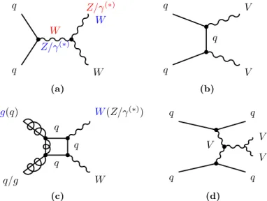
The by far dominant production process is via gluon fusion (ggF) occurring through quark loops dominated by heavy quarks, followed by the vector boson fusion (VBF) with by an order of magnitude smaller cross section. The cross sections for associated productions (V H) with vector bosons, V = W and Z, are yet further factors of two (W H ) and four (ZH) smaller than the VBF production. Production in association with a top-quark-pair occurs even less frequently. The cross sections as a function of the Higgs boson mass are shown in Fig. 2.7a. The cross section falls rapidly with increasing Higgs boson mass for all production modes. The calculations of the cross sections are described in [32]. A summary of the calculations relevant for this thesis is given below.

The ggF cross section has been computed up to NNLO in QCD [34–39] including

Chapter 2. The Higgs Boson in the Standard Model

Table 2.2: The dominant Higgs boson production processes at the LHC and their cross section at a center-of-mass energy of√s= 8 TeV for a Higgs boson mass ofmH = 125 GeV [33].

Production mode Symbol Cross section [pb] Diagram (mH = 125 GeV) (Figure)

gg

H ggF 19.52

2.6a

qq

qqH VBF 1.58

2.6b

qq

W H W H 0.70

2.6c

qq

ZH ZH 0.39

2.6c

gg

ttH ttH 0.13

2.6d

H

g g

t/b

(a)

H

q q

q q

W/Z

(b)

H

W/Z W/Z

q q

(c)

H

g g

t t

t

(d)

Figure 2.6: Leading-order Feynman diagrams for the dominant Higgs boson production mech- anisms (a) gluon fusion (ggF), (b) weak vector boson fusion (VBF), (c) associated production withW or Z bosons (V H) and (d) associated production with a top-quark-pair (ttH).

14

2.2 - Higgs Boson Production in Proton-Proton Collisions

[GeV]

MH

80 100 120 140 160 180 200

H+X) [pb] →(pp σ

10-2

10-1

1 10 102

= 8 TeV s

LHC HIGGS XS WG 2012

H (NNLO+NNLL QCD + NLO EW) pp →

qqH (NNLO QCD + NLO EW) pp →

WH (NNLO QCD + NLO EW) pp →

ZH (NNLO QCD +NLO EW) pp →

ttH (NLO QCD) pp →

(a)

[GeV]

MH

80 100 120 140 160 180 200

Higgs BR + Total Uncert [%]

10-4

10-3

10-2

10-1

1

LHC HIGGS XS WG 2013

b b

τ τ

µ µ c c

gg

γ

γ Zγ

WW

ZZ

(b)

Figure 2.7: Predictions for (a) Higgs boson production cross section for proton-proton collisions at√s= 8 TeV and (b) branching ratios for the most important Higgs boson decay channels as a function of the Higgs boson massmH (from [33]). The uncertainties are indicated as bands.

NLO electroweak (EW) corrections [40, 41] and QCD soft-gluon resummation up to next-to-next-to-leading logarithmic (NNLL) terms [42]. These calculations are detailed in [43–45] and assume factorization of QCD and EW corrections.

The VBF cross section has been computed with full NLO QCD and EW correc- tions [46–48] and approximate NNLO QCD corrections [49] and full NLO QCD and EW corrections [46–48]. The cross section for the associated V H production has been calculated using NLO QCD and approximate NNLO corrections [50, 51] and NLO EW corrections [52]. The ttH production, not relevant here due to the small cross section, has been calculated only in NLO QCD.

The uncertainties, given in Table 2.2 and indicated by the bands in Fig. 2.7a, arise from uncertainties in the PDFs as well as from uncertainties from the choice of the factorization and normalization scales [32, 53].

The production mode through vector boson fusion is the focus of this thesis. Even

though the cross section is smaller than for the dominant ggF production, it has the

advantage of a characteristic signature with additional forward jets in the final state

which can be exploited to separate the VBF production process from the background.

Chapter 2. The Higgs Boson in the Standard Model

The ggF process contributing due to its much larger cross section is considered as additional background.

The two quarks in the final state of the VBF production, remnants of the incoming protons, are produced in forward direction while the Higgs boson decay products are expected in the central region of the detector. Since quarks from the incoming protons carry larger momenta than gluons (see Fig. 2.5) the invariant mass of the two additional quarks in the VBF process is expected to be larger than for QCD background processes where predominantly gluons are emitted from the incoming quarks. Since there is no color exchange between the initial and final state particles in the lowest-order weak VBF production, hadron activity in the central region, between the two quarks is sup- pressed [54–57]. In contrast, most backgrounds as well as the ggF production are QCD processes with hadronic activity expected in the central region. The exploitation of these characteristic properties for the selection of VBF events is explained in Chapter 5.

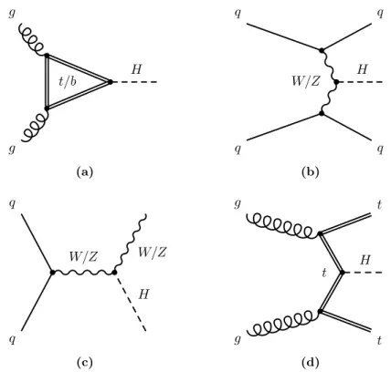
2.2.3 Higgs Boson Decays

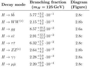
The Higgs boson, as predicted by the Standard Model, decays through many different decay modes. The Standard Model Higgs boson favors decays to heavy vector bosons and fermions. Table 2.3 lists the dominant decay modes, ordered according to their branching fractions exemplary for m

= 125 GeV. A Higgs boson with m

= 125 GeV dominantly decays into a b-quark-pair, followed by the decay into two W bosons. The decay to photons occurs predominantly via W boson and top quark loops. The H

gg decay process occurs in a similar manner via heavy quark loops like in ggF production (see Fig. 2.6a).

The sensitivity of the Higgs boson search depends not only on the branching fraction but also the final state signature and the amount of background for a particular final state. Strongly interacting decay products, such as b and c quarks, gluons or hadronic decays of W and Z bosons therefore are less sensitive final states in a hadron collider environment than final states with leptons.

When estimating the sensitivity for different Higgs boson decay channels, the subse- quent decays of unstable daughter particles, such as the massive vector bosons, have to be considered as well. The analysis in this thesis uses H

W W

`ν`ν decays where both W bosons decay leptonically. A theoretical study of this final state in combination with VBF production can be found in [59].

16

2.2 - Higgs Boson Production in Proton-Proton Collisions

Table 2.3: Overview of the dominant Higgs boson decay modes for a Higgs boson mass mH = 125 GeV [58]. Details on the branching fraction calculations can be found in [53].

Decay mode Branching fraction Diagram (mH = 125 GeV) (Figure)

H

b ¯ b 5.77

10

2.8c H

W W

2.15

10

2.8b H

gg 8.57

10

2.6a H

c¯ c 2.91

10

2.8c H

τ τ ¯ 6.32

10

2.8c H

ZZ

2.64

10

2.8b H

γγ 2.28

10

2.8a H

µ¯ µ 2.20

10

2.8c

H

γ γ

t/W

(a)

H

W/Z W/Z

(b)

H

f f

(c)

Figure 2.8:Leading-order Feynman diagrams for the main decay modes of the Standard Model Higgs boson.

Chapter 2. The Higgs Boson in the Standard Model

The

[60] program computes Higgs boson decay widths and branching ratios for all channels. All available higher-order QCD corrections are taken into account. The Monte-Carlo generator

[61, 62] simulates Higgs boson decays into four- leptons and is used for the branching fraction calculation. It takes into account all NLO QCD and electroweak corrections as well as interference terms from higher-order processes at LO and NLO, contributing to both the H

V V and the subsequent V

f f decays.

The determination of the uncertainties in the branching fraction calculations is detailed in [53]. Uncertainties in the input parameters α

and m

, m

and m

and uncertainties due to missing higher-order corrections are taken into account. Both contribute at the same level to the uncertainty in the branching ratio of dibosonic decays.

2.2.4 Event Generation and Simulation

In order to compare proton-proton collision data with theoretical predictions, large samples of simulated events are needed. The simulation proceeds in several steps, starting from the hard scattering process at the parton-level using the highest-order

(ME) calculation available. In a second step,

(PS) algorithms are used to simulate higher-order processes like gluon radiation by initial or final state particles, not taken into account in the matrix element calculation. The Monte-Carlo event generation is described in [63].

The hadronization of the final state partons is simulated using Monte-Carlo methods like the

[64]. The model parameters are tuned to electron-positron annihilation data where the hadronization process can be investigated in a clean envi- ronment.

In the last step, the underlying event is simulated. Like for the hadronization, the underlying event descriptions are tuned to data. Besides the underlying event, additional soft proton-proton interactions not involved in the hard scatter process, so called

events, discussed in Section 3.1, have to be taken into account. The simulation of the pile-up contributions is performed in the same way as it is done for the underlying event.

The presented analysis uses several Monte-Carlo generators for the simulation of the signal and background processes. An overview is given in Table 2.4. The generators are specialized either for the simulation of the hard or the soft part of the process

18

2.2 - Higgs Boson Production in Proton-Proton Collisions

Table 2.4: Overview of the Monte-Carlo event generators used in the presented analysis. The part of the event simulation the program is used for is indicated by HS for hard scattering process; had. for hadronization; PS for parton showering; UE+PU for underlying event and pile- up modelling. “All” indicates the case where the generator is used for the full event description.

Name Application Remarks

NLO

Powheg

[66] HS

[67] HS

LO

Alpgen

[68] HS

Combined with

and

using MLM [65]

matching scheme

[69] HS

MadGraph

[70–72] HS

GG2WW 3.2.1

[73, 74] HS Dedicated to gg

W W

[75] All Includes higher-order

electroweak corrections

[76, 77] had., PS, UE+PU Also for qq

V H HS

[78] had., PS

Jimmy

[79] UE+PU Combined with

and, therefore, are combined for the full event simulation. Most generators only include leading-order calculations. The

generator used for the signal simulation takes next-to-leading order corrections into account. The

generator is based only on leading-order ME calculations but employs the MLM scheme [65] to match parton shower contributions generated by the

program to the matrix-element calculations in an optimal way.

The generators used for simulation of the hard scattering process need Parton Dis-

tribution Functions (PDF) as input. The

and

generators use the

PDF set of CT10 [29] while the

,

and

generators use

the PDF set of CTEQ6L1 [30].

Chapter 2. The Higgs Boson in the Standard Model

2.3 Higgs Boson Properties

The Standard Model Higgs boson is a scalar CP-even particle, i.e. J

= 0

where J denotes the spin and P the parity. Furthermore, all couplings of the Higgs boson to Standard Model particles are determined, and can be tested experimentally. The mass of the Higgs boson is not predicted by the Standard Model. However, upper limits on the Higgs boson mass arise from the requirement of unitarity in W W scattering amplitudes (m

870 [80]), from the requirement of perturbativity of the branching fraction calculation of H

V V

decays (m

700 GeV [81]) as well as from constraints due to quadratic Higgs boson self coupling terms leading to a divergence (Landau pole) at a scale depending on the Higgs boson mass ( m

170 [82]). A lower bound on the Higgs boson mass arises from the claim for a stable vacuum (m

> (129.4

1.8) GeV

[83]). The constraints arising from Higgs boson self coupling terms and from the vacuum stability claim assume no new physics up to the Planck scale (M

2

10

GeV). In addition electroweak precision measurements, sensitive to the Higgs boson mass through higher- order corrections, are best compatible with a Higgs boson with m

= 94

GeV [84].

Since the startup of the LHC the Higgs boson has been searched for extensively by the LHC experiments ATLAS and CMS. In the higher mass range (m

2

m

) the decays into W and Z boson pairs are most sensitive for Higgs boson searches due to the large branching fractions (see Fig. 2.7b) while in the lower mass range (m

2

m

) despite the small branching fraction decays into two photons provide the highest sensitivity due to the very clean signature and high Higgs boson mass resolution.

Already in July 2012 the ATLAS [5] and CMS [6] experiments observed a significant excess of events, well compatible with the expectations for a Standard Model Higgs boson with a mass around 125 GeV, with a fraction of the full dataset (5 fb

at

s = 7 TeV and 5.8 fb

at

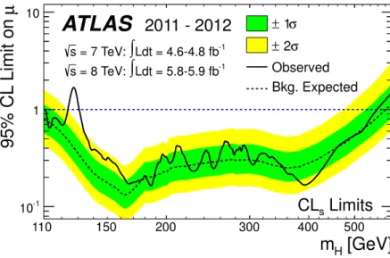
s = 8 TeV). Except for a small mass region around 125 GeV a Standard Model Higgs boson is excluded (see Fig. 2.9) in the mass region favored by theoretical and electroweak precision measurement constraints. Once the full dataset was analyzed the excluded mass region was extended to 110–123 GeV and 127–710 GeV [5, 85–88].

Employing the full available dataset measurements in the most sensitive decays to

∗The measured Higgs boson mass (mH= (125.5±0.6) GeV [7] andmH= (125.7±0.4) GeV [8]) is in contradiction to this constraint with a significance of two standard deviations. In case of confirmation with higher precision this leads to the conclusion that either there has to be new physics before the Planck scale or the vacuum is meta-stable. The lifetime of the meta-stable vacuum could, however, be longer than the age of the universe [82].

20

2.3 - Higgs Boson Properties

[GeV]

m

200 300 400 500

µ 9 5 % C L L im it o n

10-1

1

10 ± 1σ

σ

± 2

Observed Bkg. Expected

ATLAS 2011 - 2012

Ldt = 4.6-4.8 fb-1

∫

= 7 TeV:

s

Ldt = 5.8-5.9 fb-1

∫

= 8 TeV:

s

Limits CL

110 150

Figure 2.9: Exclusion limit at 95% confidence level as a function of the Higgs boson mass, mH. The observed limit (solid line) is compared to the limit expected from the background-only hypothesis (dashed line) including the±1σ(green) and±2σ(yellow) uncertainty bands in the expectation (from [5]).

two photons by the ATLAS [89] experiment, and two Z bosons by the ATLAS [86] and CMS [90] experiments show discovery-level signal significances with over six standard deviations, while the diphoton channel measurement by the CMS [87] experiment shows a significance of 3.2 standard deviations. These two channels additionally provide a precise measurement of the Higgs boson mass by means of the invariant mass computed from the final state particle four-momenta. Combining the two mass measurements a value of m

= (125.5

0.6) GeV [7] and m

= (125.7

0.4) GeV [8] is found by the ATLAS and CMS experiments, respectively.

Evidence, with roughly four standard deviation significance is found for the decays into two W bosons [91, 92] and two τ leptons [93, 94]. The former will be discussed in detail in Chapters 5 and 6. The latter is of particular interest since the coupling of the Higgs boson to leptons is directly confirmed. Indirect confirmation of the Yukawa coupling of the quark sector is given by the production via gluon fusion. No significant signal, i.e. with above three standard deviations, is yet observed in the decay modes to b quarks [95, 96] and muons [97, 98].

An important test to identify the new boson as the Standard Model Higgs boson is

Chapter 2. The Higgs Boson in the Standard Model

the measurement of spin and parity which are investigated in angular distributions of final state particles. The most sensitive Higgs boson decay channel is H

ZZ

4`

where the final state can be fully described by six angles defined between the final state leptons as well as between the leptons and the beam axis. Those angles are sensitive to spin and parity of the Higgs boson. For the measurement of the spin also the H

γγ and H

W W

channels can be used. The spin-1 hypothesis is excluded already by the observation of the decays to two photons with spin-1 and zero mass because of the Landau-Yang theorem [99,100]. Evidence against eigenstates J

= 1

, 1

, 2

is found at a significance level of three standard deviations and the odd-parity eigenstate 0

is disfavored at a level of two standard deviations [90, 102].

The Higgs boson mass, spin, parity and decay rates have been measured as well as the couplings of the Higgs boson to Standard Model particles and the different production mechanisms. The latter two are described in Chapter 6. All measurements show good agreement with the Standard Model predictions and the results of the ATLAS and CMS experiments are well compatible with each other.

∗A large number of spin-2 models are possible. A specific one, corresponding to a graviton-inspired tensor with minimal couplings to Standard Model particles is investigated by ATLAS and CMS as described in [101].

22

Chapter 3

The ATLAS Detector at the Large Hadron Collider

The Large Hadron Collider (LHC) is a proton storage ring with 27 km circumference located at the European Organization for Nuclear Research CERN which collides proton beams circulating in opposite directions. It was designed to provide collision energies and beam intensities sufficient for either the discovery or the exclusion of the Standard Model Higgs boson. The technologies needed to reach this goal, are summarized in Section 3.1 following the detailed description in [103–106].

The LHC provides proton-proton collisions for several experiments. The main ones are ATLAS [107], CMS [108], LHCb

[109] and ALICE

[110]. LHCb is dedicated to heavy flavor physics while ALICE studies the quark-gluon-plasma using special fills of the LHC with lead ions. ATLAS and CMS are multi-purpose experiments, dedicated to the search for the Higgs boson and for new physics beyond the Standard Model. The ATLAS detector, which delivered the data for the presented analysis, will be described in Section 3.2.

3.1 The Large Hadron Collider

The LHC physics goals require large collision energy since the cross sections of processes of interest, such as Higgs boson productions, raise faster with increasing collision energy compared to the cross sections of most background processes (see Fig. 2.3). Since the processes of interests are rare, many collision events are needed to gain statistical

∗LHCb: Large Hadron Collider Beauty

†ALICE: A Large Ion Collider Experiment

Chapter 3. The ATLAS Detector at the Large Hadron Collider

significance. This requires high beam intensity. The LHC collides proton beams in the tunnel of the former LEP electron-positron collider [111, 112] using superconducting dipole magnets to keep the protons on their orbits.

The protons are pre-accelerated before injected into the LHC as illustrated in Fig. 3.1.

Linac 2

accelerates the protons to 50 MeV before they are injected into the

which accelerates them further to 1.4 GeV. The

(PS) increases the energy to 25 GeV and the

(SPS) to 450 GeV. The protons are then injected into the LHC in two opposite directions where they are accelerated to their final energies. The maximum design energy is 7 TeV per beam.

The pre-acceleration stages provide protons in bunches. The LHC is designed to accelerate up to n

= 2835 bunches per beam with N

10

protons per bunch and collisions every 25 ns. The event rate, dN/dt = L σ, for a given process with cross section σ is determined by the instantaneous luminosity L, which depends on the beam parameters:

L = N

n

f

γ

4π

β

F , (3.1)

where f

is the revolution frequency of the protons, γ

their relativistic gamma-factor,

the beam emittance, β

the transverse beam amplitude at the interaction point and F a geometric reduction factor taking into account that the beams cross under an angle.

The design peak luminosity of the LHC is 10

s

cm

. However, not all beam parameters have reached their design values in the past years. In the year 2011, the LHC was running with a beam energy of 3.5 TeV which was increased to 4 TeV in 2012.

The number of bunches per beam was increased from 200 to 1380 during 2011 and kept at 1380 in 2012. Peak luminosities of about 4

10

s

cm

and 8

10

s

cm

have been reached in 2011 and 2012, respectively.

The physics program relies on the

luminosity

=

L dt collected over time. The integrated luminosities delivered by the LHC and recorded by the ATLAS detector are shown in Fig. 3.2a. An integrated luminosity of 5.46 fb

was delivered by the LHC at a collision energy of 7 TeV in the year 2011 of which 4.57 fb

were recorded by ATLAS and classified as good quality data. In the year 2012 an integrated luminosity of 22.8 fb

was delivered by the LHC at a collision energy of 8 TeV of which 20.3 fb

were recorded under good conditions by the ATLAS detector.

For a given peak luminosity, the expected number of inelastic proton-proton inter- actions per bunch crossing can be calculated from the total inelastic cross section σ

24

3.1 - The Large Hadron Collider

Figure 3.1: Illustration (from [113]) of the CERN accelerator system. The acceleration chain starts with Linac 2 and is followed by the acceleration in the booster. The protons are then accelerated further by theProton Synchrothron (PS) and theSuper Proton Synchrotron (SPS) before they are injected into the LHC.

Chapter 3. The ATLAS Detector at the Large Hadron Collider

shown in Fig. 2.3. For the design parameters of the LHC and the ones used in the years 2011 and 2012, the expected numbers of inelastic proton-proton interactions per bunch crossing are 23, 9 and 20, respectively. The distributions of the mean numbers of interactions per bunch crossing measured by the ATLAS detector in 2011 and 2012 are shown in Fig. 3.2b.

The rates of most processes of interest, such as Higgs boson production, are small (see Fig. 2.3). The processes of interest are therefore accompanied by additional inelastic proton-proton interactions in the same event due to the large inelastic cross section.

These contributions to the event are referred to as

inelastic proton-proton interaction occurred in the same bunch crossing. In particular for 25 ns bunch spacing, also proton-proton interactions from previous bunch crossings contribute which is referred to as

γ-rays from interactions of protons produced in collisions with the detector material, referred to as

In-time pile-up has by far the largest impact on the physics analyses.

Month in Year Jan Apr Jul Oct Jan Apr Jul Oct

-1fbTotal Integrated Luminosity

0 5 10 15 20 25 30

ATLAS Preliminary

= 7 TeV s 2011,

= 8 TeV s 2012, LHC Delivered

ATLAS Recorded Good for Physics

fb-1 Delivered: 5.46

fb-1 Recorded: 5.08

fb-1 Physics: 4.57

fb-1 Delivered: 22.8

fb-1 Recorded: 21.3

fb-1 Physics: 20.3

(a)

Mean Number of Interactions per Crossing

0 5 10 15 20 25 30 35 40 45

/0.1]-1Recorded Luminosity [pb

0 20 40 60 80 100 120 140 160

180 ATLASOnline Luminosity

> = 20.7 , <µ Ldt = 21.7 fb-1

∫

= 8 TeV, s

> = 9.1 µ , <

Ldt = 5.2 fb-1

∫

= 7 TeV, s

(b)

Figure 3.2: (a) Total integrated luminosity delivered by the LHC (green), recorded by ATLAS (yellow) and classified as good quality data (blue) at√s= 7 TeV and√s= 8 TeV in 2011 and 2012, respectively. (b) Luminosity weighted distributions of the mean number of interactions per bunch crossing for 2011 and 2012. The figures are from [114].

26