Evidence for Higgs boson Yukawa couplings in the H → ττ decay mode with the ATLAS detector

A TLAS-CONF-2014-061

ATLAS NOTE

ATLAS-CONF-2014-061

October 7, 2014

Evidence for Higgs boson Yukawa couplings in the H → ττ decay mode with the ATLAS detector

The ATLAS Collaboration

Abstract

Results of a search for H → ττ decays are presented, based on the full set of proton- proton collision data recorded by the ATLAS experiment at the LHC during 2011 and 2012.

The data correspond to integrated luminosities of 4.5 fb

and 20.3 fb

at centre-of-mass energies of √

s = 7 TeV and √

s = 8 TeV respectively. All combinations of leptonic (τ → `ν¯ ν with ` = e, µ) and hadronic (τ → hadrons ν) tau decays are considered. An excess of events over the expected background from other Standard Model processes is found with an observed (expected) significance of 4.5 (3.5) standard deviations. This excess provides evidence for the direct coupling of the recently discovered Higgs boson with mass m

=125 GeV to fermions. The measured signal strength, normalised to the Standard Model expectation, of µ = 1.42

is consistent with the predicted Yukawa coupling strength in the Standard Model.

c

Copyright 2014 CERN for the benefit of the ATLAS Collaboration.

Reproduction of this article or parts of it is allowed as specified in the CC-BY-3.0 license.

1 Introduction

The investigation of the origin of electroweak symmetry breaking and, related to this, the experimen- tal confirmation of the Brout-Englert-Higgs mechanism [1–6] is one of the prime goals of the physics programme at the Large Hadron Collider (LHC) [7]. With the discovery of a Higgs boson with a mass of approximately 125 GeV by the ATLAS [8] and CMS [9] Collaborations, an important milestone has been reached. More precise measurements of the properties of the discovered particle [10, 11] as well as tests of the spin-parity quantum numbers [12, 13] have strengthened the hypothesis of its consistency with the Standard Model (SM) Higgs boson.

These measurements rely predominantly on studies of the bosonic decay modes, H → γγ, H → ZZ

and H → WW

. To establish the mass generation for fermions as implemented in the SM, it is of prime importance to demonstrate the direct coupling of the Higgs boson to fermions and its proportionality to mass [14]. The most prominent candidate decay modes are the decays into tau leptons, H → ττ, and bottom quarks (b-quarks), H → b b. The search for decays to ¯ b b ¯ requires the restriction to Higgs bosons produced in association with vector bosons or t¯ t pairs, and by vector-boson fusion. The smaller rate of these processes in the presence of still large background makes their detection challenging. More favourable signal-to-background conditions are expected for H → ττ decays. Recently, the CMS Collab- oration has published evidence for H → ττ at a significance of three standard deviations (σ) [15] and an excess of events above the expected background corresponding to a significance of 2.1σ in the search for H → b b ¯ decays [16] for a Higgs boson mass, m

, of 125 GeV. The combination of the channels, based on a dataset corresponding to integrated luminosities of 5 fb

at a centre-of-mass energy of √

s = 7 TeV and ∼20 fb

at √

s = 8 TeV, provides evidence for fermionic couplings of the newly discovered Higgs boson with a significance of 3.8σ [17]. Recently, the ATLAS Collaboration has observed an excess of events above the expected background in the search for H → b b ¯ decays [18] corresponding to a signifi- cance of 1.4σ for m

= 125 GeV, based on the full dataset. In the search for H → ττ decays, the ATLAS Collaboration has set upper limits on the cross section times the branching ratio, normalised to the SM prediction, between 2.9 and 11.7 in the mass range 100–150 GeV from 4.7 fb

of data collected at

√ s = 7 TeV [19].

In this note, the results of a search for H → ττ decays are presented, based on the full proton–proton dataset collected by the ATLAS experiment during the 2011 and 2012 data taking periods, correspond- ing to integrated luminosities of 4.5 fb

at a centre-of-mass energy of √

s = 7 TeV and 20.3 fb

at

√ s = 8 TeV. All combinations of leptonic (τ → `ν¯ ν with ` = e, µ) and hadronic (τ → hadrons ν) tau decays are considered.

The corresponding three analysis channels are denoted as τ

τ

, τ

τ

, and τ

τ

in the following. The search is designed to be sensitive to the major production processes of a SM Higgs boson, i.e. production via gluon fusion (ggF) [20], vector-boson fusion (VBF) [21], and the associated production (V H) with V = W or Z. These production processes lead to different final state signatures, which have been exploited by defining an event categorisation. Two dedicated categories are considered to achieve both a good signal-to-background ratio and a good resolution for the reconstruc- tion of the ττ invariant mass. The VBF category, enriched in events produced via vector-boson fusion, is defined by the presence of two jets with a large separation in pseudorapidity.

The Boosted category contains events with a large transverse momentum of the reconstructed Higgs boson candidate. It is dominated by events produced via gluon fusion with additional jets from gluon radiation. In view of the signal-to-background conditions, and in order to exploit correlations between final state observables,

1Throughout this paper the inclusion of charge-conjugate decay modes is implied.

2The ATLAS experiment uses a right-handed coordinate system with its origin at the nominal interaction point (IP) in the centre of the detector and thez-axis along the beam direction. Thex-axis points from the IP to the centre of the LHC ring, and they-axis points upward. Cylindrical coordinates (r, φ) are used in the transverse (x, y) plane,φbeing the azimuthal angle around the beam direction. The pseudorapidity is defined in terms of the polar angleθasη=−ln tan(θ/2). The distance∆Rin theη−φspace is defined as∆R=p

(∆η)²+(∆φ)².

a multivariate analysis technique, based on boosted decision trees (BDTs) [22–24], is used to extract the final results. As a cross-check, a separate analysis where cuts on kinematic variables are applied is carried out.

2 The ATLAS detector and object reconstruction

The ATLAS detector [25] is a multi-purpose detector with a cylindrical geometry. It comprises an in- ner detector (ID) surrounded by a thin superconducting solenoid, a calorimeter system and an extensive muon spectrometer embedded in a toroidal magnetic field. The ID tracking system consists of a silicon pixel detector, a silicon microstrip detector (SCT), and a transition radiation tracker (TRT). It provides precise position and momentum measurements for charged particles and allows e ffi cient identification of jets containing b-hadrons in the pseudorapidity range |η| < 2.5. The ID is immersed in a 2 T axial magnetic field and is surrounded by high granularity lead/liquid-argon (LAr) sampling electromagnetic calorimeters which cover the pseudorapidity range |η| < 3.2. An iron / scintillator tile calorimeter provides hadronic energy measurements in the central pseudorapidity range (|η| < 1.7). In the forward regions (1.5 < |η| < 4.9), the system is complemented by two end-cap calorimeters using LAr as active material and copper or tungsten as absorbers. The muon spectrometer (MS) surrounds the calorimeters and con- sists of three large superconducting eight-coil toroids, a system of tracking chambers, and detectors for triggering. The deflection of muons is measured within |η| < 2.7 by three layers of precision drift tubes, and cathode strip chambers in the innermost layer for |η| > 2.0. The trigger chambers consist of resistive plate chambers in the barrel (|η| < 1.05) and thin-gap chambers in the end-cap regions (1.05 < |η| < 2.4).

A three-level trigger system [26] is used to select events. A hardware-based Level-1 trigger uses a subset of detector information to reduce the event rate to a value of at most 75 kHz. The rate of accepted events is then reduced to about 400 Hz by two software-based trigger levels, Level-2 and the Event Filter.

The reconstruction of the basic physics objects used in this analysis is described in the following.

The primary vertex is selected by choosing the vertex candidate with the highest sum of the squared transverse momentum of all tracks matched to the candidate.

Electron candidates are reconstructed from energy clusters in the electromagnetic calorimeters matched to a track in the ID. They are required to have an energy in the transverse plane E

> 15 GeV, be within the pseudorapidity range |η| < 2.47 and pass the medium shower shape and track selection criteria de- fined in Ref. [27]. Candidates found in the calorimeter transition region (1.37 < |η| < 1.52) are not considered. Typical reconstruction and identification efficiencies for electrons passing these selection cuts range between 80% and 90% depending on E

and η.

Muon candidates are reconstructed using an algorithm [28] that combines information from the ID and the MS. They are required to have a momentum in the transverse plane p

> 10 GeV and to be within |η| < 2.5. Typical e ffi ciencies for muons passing these selection criteria are above 95% [29].

Jets are reconstructed using the anti-k

jet clustering algorithm [30, 31] with a radius parameter R = 0.4, taking topological energy clusters [32] in the calorimeters as inputs. Jet energies are corrected for the contribution of pile-up interactions using a jet-area based technique [33] and are calibrated using p

and η dependent correction factors determined from simulation and data [34–36]. Jets are required to be reconstructed in the range |η| < 4.5 and to have p

> 30 GeV. To reduce the contamination of jets from multiple interactions in the same or neighbouring bunch crossings (pile-up), for jets with |η| < 2.4, the scalar sum of the p

of tracks matched to jets and originating from the primary vertex is required to be at least 75% (50%) of the scalar sum of the transverse momenta of all tracks in the jet for the 7 TeV (8 TeV) dataset (jet vertex fraction, JVF). Moreover, for the 8 TeV dataset, the JVF selection is applied only to jets with p

< 50 GeV. Jets with no associated tracks are retained.

In the pseudorapidity range |η| < 2.5, b-jets are selected using a tagging algorithm [37]. The b-

jet tagging algorithm used has an efficiency of 60–70% for b-jets in simulated t¯ t events [38]. The

corresponding light-quark jet misidentification probability is 0.1–0.5%, depending on the jet p

and η [39].

Hadronically decaying tau leptons are reconstructed starting from clusters of energy in the elec- tromagnetic and hadronic calorimeters. The τ

reconstruction is seeded by the anti-k

jet finding algorithm with a radius parameter R = 0.4. Tracks in a cone of radius ∆ R < 0.2 from the cluster barycen- tre are associated to the τ

candidate, and the τ

charge is determined from the sum of the charges of the tracks. The rejection against jets is provided in a separate identification step using discriminating variables based on tracks with p

> 1 GeV and calorimeter cells found in the core region ( ∆ R < 0.2) and in the region 0.2 < ∆ R < 0.4 around the τ

candidate direction. Such discriminating variables are combined in a boosted decision tree and three working points, labelled tight, medium and loose [40], are defined, corresponding to di ff erent τ

identification e ffi ciency values.

In this analysis, τ

candidates with p

> 20 GeV and |η| < 2.47 are used. The τ

candidates are required to have charge ±1, and must be 1- or 3-track (prong) candidates. In addition, a two-track sample (where the charge requirement is dropped) is retained for background studies, as described in Section 6.2. The identification e ffi ciency for τ

candidates passing the medium identification criteria is of the order of 55–60%. Dedicated criteria [40] to separate τ

candidates from misidentified electrons are also applied, with a selection e ffi ciency for true τ

decays of 95%. The probability to misidentify a jet with p

> 20 GeV as a τ

candidate is typically 1–2%.

Following their reconstruction, candidate leptons, hadronically decaying taus and jets may point to the same energy deposits in the calorimeters (within ∆ R < 0.2). Such overlaps are resolved by selecting in the order of priority muons, electrons, τ

, and jet candidates. For all channels, the leptons that are considered for overlap removal with τ

candidates need only to satisfy looser criteria than those defined above, to reduce misidentified τ

candidates from leptons. The p

threshold of muons considered for overlap removal is also lowered to 4 GeV.

The missing transverse momentum (E

) is reconstructed using the energy deposits in calorimeter cells calibrated according to the reconstructed physics objects (e, γ, τ

, jets and µ) to which they are associated [41]. The transverse momenta of reconstructed muons are included in the E

calculation, with the energy deposited by these muons in the calorimeters taken into account. The energy from calorimeter cells not associated with any other objects is scaled by the soft-term vertex fraction and also included in the E

calculation. This fraction is the ratio of the scalar sum of the p

of tracks from the primary vertex unmatched to objects to the scalar sum p

of all tracks in the event also unmatched to objects. This method allows a better reconstruction of the E

in high pile-up conditions [42].

3 Data and simulated samples

After data quality requirements, the integrated luminosities of the samples used are 4.5 fb

at √

s = 7 TeV and 20.3 fb

at √

s = 8 TeV.

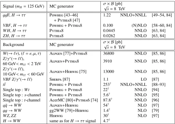
Samples of signal and background events were simulated using various Monte Carlo (MC) genera- tors, as summarised in Table 1. The generators used for the simulation of the hard scattering process and the model used for the simulation of the parton shower, of the hadronisation and of the underlying event activity are listed. In addition, the cross-section values to which the simulation is normalised and the perturbative order in QCD of the respective calculations are given.

The signal contributions considered include the three main processes for Higgs boson production at the LHC: the gluon fusion (ggF), the vector-boson fusion (VBF), and the associated V H production processes. The contributions from the associated t¯ tH production have been found to be small and are neglected. The gluon fusion and the VBF production are simulated with P owheg [43–46] interfaced to

3In the following, theτhadsymbol always refers to the visible decay product of theτhadronic decay.

P ythia 8 [47]. In the P owheg event generator the CT10 [48] parametrisation of the parton density func- tions (PDFs) is used. The overall normalisation of the ggF process is taken from a calculation at next- to-next-to-leading order (NNLO) [49–54] in QCD, including soft-gluon resummation up to the order of next-to-next-to-leading logarithm (NNLL) [55]. Next-to-leading order (NLO) electroweak (EW) correc- tions are also included [56, 57]. The VBF production is normalised to a cross section calculated with full NLO QCD and EW corrections [58–60] with an approximate NNLO QCD correction applied [61].

The associated V H production process is simulated with P ythia 8. The C teq 6L1 [62] parametrisation of PDFs is used for the P ythia 8 event generator. The predictions for V H production are normalised to cross sections calculated at NNLO in QCD [63], with NLO EW radiative corrections [64] applied.

Additional corrections to the shape of the generated p

distribution of Higgs bosons produced via gluon fusion are applied to match the distribution from a calculation at NNLO including the NNLL corrections provided by the HRes2.1 [65] program. In this calculation, the effects of finite masses of the top and bottom quarks [65, 66] are included and dynamical renormalisation and factorisation scales, µ

, µ

= q

m

+ p

, are used. A reweighting is performed separately for events with less than or equal to one jet at particle level and for events with two or more jets. In the latter case, the Higgs boson p

spectrum is reweighted to match the M in L o HJJ predictions [67]. The reweighting is derived such that the inclusive Higgs boson p

spectrum and the p

spectrum of events with at least two jets matches the HR es 2.1 and M in L o HJJ predictions respectively, and that the jet multiplicities are in agreement with (N)NLO calculations from J et VH eto [68–70].

The NLO EW corrections for the VBF production depend on the p

of the Higgs boson, varying from a few percent at low p

to ∼ 20% at p

= 300 GeV [71]. The VBF-produced Higgs boson p

spectrum is therefore reweighted, based on the di ff erence between the P owheg+ P ythia and the H awk [58, 59]

calculation, which includes these corrections.

The main and largely irreducible Z/γ

→ ττ background is modelled using Z/γ

→ µµ events from data,

where the muon tracks and associated energy depositions in the calorimeters are replaced by the corresponding simulated signatures of the final state particles of the tau decay. In this approach, essential features such as the modelling of the kinematics of the produced boson, the modelling of the hadronic activity of the event (jets and underlying event) as well as contributions from pile-up are taken from data.

Thereby the dependence on the simulation is minimised and only the τ decays and the detector response of the tau-lepton decay products are based on simulation. By requiring two isolated, high-energy muons with opposite charge and a dimuon invariant mass m

> 40 GeV, Z → µµ events can be selected from the data with high efficiency and purity. In order to replace the muons in the selected events, all tracks associated to the muons are removed and calorimeter cell energies associated to the muons are corrected by subtracting the corresponding energy depositions for a single simulated Z → µµ event with the same kinematics. Finally, both the track information and the calorimeter cell energies of a simulated Z → ττ decay are added to the data event. The decays of the tau leptons are simulated by T auola [72], matched to the kinematics of the muons in data they replace, including polarisation and spin correlations [73], and accounting for the mass di ff erence between the muons and the tau leptons. This hybrid sample is referred to as embedded data in the following.

Other background processes are simulated using di ff erent generators, each interfaced to P ythia [47, 74] or H erwig [75] to provide the parton shower, hadronisation and the modelling of the underlying event, as indicated in Table 1. For the Herwig samples, the decays of tau leptons are simulated using T auola [72]. P hotos [76] provides photon radiation from charged leptons for all samples. The samples for W /Z + jets production are generated with A lpgen [77], employing the MLM matching scheme [78]

between the hard process (calculated with LO matrix elements for up to five jets) and the parton shower.

For WW production the loop-induced gg → WW process is also generated using the gg 2WW [79]

4These processes are hereafter for simplicity denoted asZ→ττandZ→µµrespectively, even though the whole contin- uum above and below theZpeak is considered.

Signal (m

125 GeV) MC generator

[pb]

s=

8 TeV

ggF,H→ττ

P

[43–46] 1.22 NNLO

NNLL [49–54, 84]

+

P

8 [47]

VBF,H→ττ

P

P

8 0.100 (N)NLO [58–60, 84]

W H,H→ττ

P

8 0.0445 NNLO [63, 84]

ZH,H→ττ

P

8 0.0262 NNLO [63, 84]

Background MC generator

[pb]

s=

8 TeV

W(→`ν), (`=e, µ, τ)

A

[77]

P

8 36800 NNLO [85, 86]

Z/γ^∗

(→

A

P

8 3910 NNLO [85, 86]

60 GeV<

2 TeV

(

A

H

[75] 13000 NNLO [85, 86]

10 GeV<

60 GeV

VBF Z/γ^∗

(→

S

[87] 1.1 LO [87]

tt

¯ P

P

8 253

NNLO

NNLL [88–93]

Single top :

P

P

8 22

NNLO [94]

Single top :

P

P

8 5.6

NNLO [95]

Single top :

AcerMC [80]

P

6 [74] 87.8

NNLO [96]

qq

¯

A

H

54

NLO [97]

gg→WW

gg2WW [79]

H

1.4

NLO [79]

WZ,ZZ

H

30

NLO [97]

H→WW

same as for

signal 4.7

Table 1: Monte Carlo generators used to model the signal and background processes at √

s = 8 TeV.

The cross sections times branching fractions (σ × B ) used for the normalisation of some processes (many of these are subsequently normalised to data) are included in the last column together with the QCD perturbative order of the calculation. For the signal processes the H → ττ branching ratio is included, and for the W and Z/γ

background processes the branching ratios for leptonic decays (` = e, µ, τ) of the bosons are included. For all other background processes inclusive cross sections are quoted (marked with a †).

program. In the A cer MC [80], A lpgen , and H erwig event generators the C teq 6L1 parametrisation of the PDFs is used, while the CT10 parametrisation is used for the generation of events with gg2WW. The normalisation of these background contributions is either estimated from control regions using data, as described in Section 6, or the cross sections quoted in Table 1 are used.

For all samples, a full simulation of the ATLAS detector response [81] using the G eant 4 program [82]

was performed. In addition, events from minimum bias interactions were simulated using the AU2 [83]

tuning of Pythia8. They are overlaid on the signal and background simulated events according to the luminosity profile of the recorded data. The contributions from these pile-up interactions are simulated both within the same bunch crossing as the hard-scattering process and in neighbouring bunch crossings.

Finally, the resulting simulated events are processed through the same reconstruction programs as the

data.

Trigger

Trigger Analysis level thresholds [GeV]

level √

s=7 TeV thresholds,

pT[GeV] τlepτlep τlepτhad τhadτhad

Single electron 20−22 eµ: pT(e)>22−24 eτ: pT(e)>25 pT(µ)>10 pT(τ)>20 – Single muon 18 µµ: pT(µ1)>20

µτ: pT(µ)>22 pT(µ2)>10 pT(τ)>20 – Di-electron 12/12 ee: pT(e1)>15

– –

pT(e2)>15

Di-τhad 29/20 – – ττ: pT(τ1)>35

pT(τ2)>25 Trigger

Trigger Analysis level thresholds [GeV]

level √

s=8 TeV thresholds,

pT[GeV] τlepτlep τlepτhad τhadτhad

Single electron 24

eµ: pT(e)>26

eτ: –

pT(µ)>10 pT(e)>26 ee: pT(e1)>26 pT(τ)>20

pT(e2)>15

Single muon 24 – µτ: pT(µ)>26

pT(τ)>20 – Di-electron 12/12 ee: pT(e1)>15

– –

pT(e2)>15 Di-muon 18/8 µµ: pT(µ1)>20

– –

pT(µ2)>10 Electron+muon 12/8 eµ: pT(e)>15

– –

pT(µ)>10

Di-τhad 29/20 – – ττ: pT(τ1)>35

pT(τ2)>25

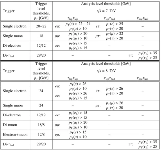
Table 2: Summary of the triggers used to select events for the di ff erent analysis channels at the two centre-of-mass energies. Both the transverse momentum thresholds applied at trigger level as well as in the analysis are listed. When more than one trigger is used, a logical OR is taken and the trigger e ffi ciencies are calculated accordingly.

4 Event selection and categorisation

4.1 Event selection

Single lepton, dilepton and di-hadronic tau triggers were used to select the events for the analysis. A summary of the triggers used by each channel at the two centre-of-mass energies is reported in Table 2.

Due to the increasing luminosity and the di ff erent pile-up conditions, the online p

thresholds increased during data taking and more stringent identification requirements were applied for the data taking at

√ s = 8 TeV in 2012. The p

requirements on the objects in the analysis are usually 2 GeV higher than the trigger requirements, to ensure that the trigger is fully e ffi cient.

In addition to applying criteria to ensure that the detector was functioning properly, requirements to increase the purity and quality of the data sample are applied by rejecting non-collision events such as cosmic rays and beam halo events. At least one reconstructed primary vertex is required with at least four associated tracks and a position consistent with the beam spot.

With respect to the object identification requirements described in Section 2, tighter criteria are ap-

plied to address the different background contributions and compositions in the different analysis chan-

nels. Higher p

thresholds are applied to electrons, muons, and τ

candidates according to the trigger

τ

τ

τ

τ

Electrons

7 TeV I( p

, 0.4) < 0.06 I( p

, 0.4) < 0.06 I (E

, 0.2) < 0.08 I(E

, 0.2) < 0.06 8 TeV I( p

, 0.4) < 0.17 I( p

, 0.4) < 0.06 I (E

, 0.2) < 0.09 I(E

, 0.2) < 0.06

Muons

7 TeV I( p

, 0.4) < 0.06 I( p

, 0.4) < 0.06 I (E

, 0.2) < 0.04 I(E

, 0.2) < 0.06 8 TeV I( p

, 0.4) < 0.18 I( p

, 0.4) < 0.06 I (E

, 0.2) < 0.09 I(E

, 0.2) < 0.06

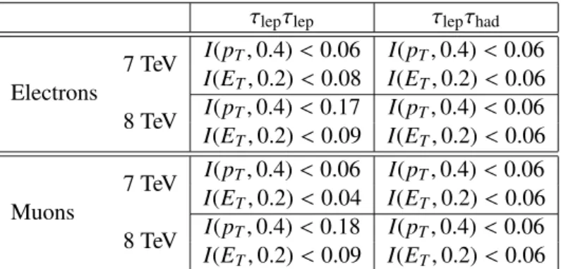
Table 3: Summary of isolation requirements applied for the selection of isolated electrons and muons at the two centre-of-mass energies. The isolation variables are defined in the text.

conditions satisfied by the event, as listed in Table 2. For the channels involving leptonic tau decays, τ

τ

and τ

τ

, additional isolation criteria on electrons and muons, based on tracking and calorime- ter information, are used to suppress the background from misidentified jets or from semileptonic decays of charm and bottom hadrons. The calorimeter isolation variable I(E

, ∆ R) is defined as the sum of the total transverse energy in the calorimeter in a given cone of size ∆ R around the electron cluster or the muon track, divided by the E

of the electron cluster or the p

of the muon respectively. The track-based isolation I( p

, ∆ R) is defined as the sum of the transverse momenta of tracks within a cone of ∆ R around the electron or muon track, divided by the E

of the electron cluster or the muon p

respectively. The isolation requirements applied are slightly different for the two centre-of-mass energies and are listed in Table 3.

In the τ

τ

channel, isolated taus are defined, if no tracks with p

> 0.5 GeV are found in an isolation region of 0.2 < ∆ R < 0.6 around the tau direction. This requirement leads to a 12% (4%) e ffi ciency loss for hadronic taus, while 30% (10%) jet rejection is obtained in 8 (7) TeV data.

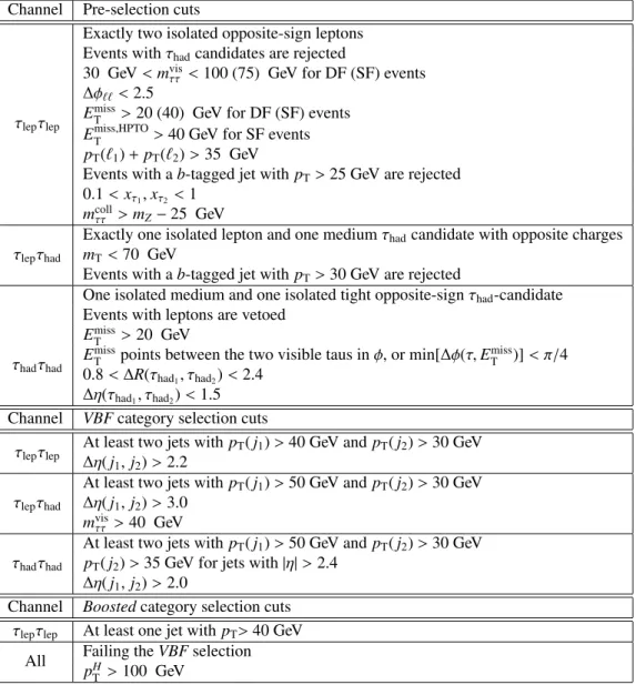
After the basic lepton selection further channel-dependent cuts are applied, as detailed in the follow- ing. The full event selection is summarised in Table 4.

τ

τ

channel: Exactly two isolated leptons with opposite-sign (OS) electric charges, passing the p

threshold listed in Table 2, are required. Events containing a τ

candidate are vetoed. For the τ

candidates considered the criteria used to reject electrons misidentified as τ

candidates are tightened to a working-point of 85% signal e ffi ciency [40].

In addition to the irreducible Z → ττ background, sizeable background contributions from Z → ``

and from t¯ t production are expected in this channel. Background contributions from Z decays, but also from charmonium and bottomonium resonances, are rejected by requirements on the invariant mass m

of the visible tau decay products, on the angle ∆ φ

between the two leptons in the transverse plane and on the missing transverse momentum E

. In order to reject the large Z → `` contribution in events with same-flavour (SF) leptons (ee, µµ) more stringent cuts on the visible mass and on E

are applied for these events than for events with di ff erent-flavour (DF) leptons (eµ). For SF final states, an additional variable named High p

Objects E

(E

) is also used to reject background from Z/γ

production. It is calculated from the high p

objects in the event, i.e. from the two leptons and jets with p

> 25 GeV. Due to the presence of real neutrinos, the two E

variables are strongly correlated for signal events but only loosely correlated for background from Z → ee and Z → µµ decays.

To further suppress background contributions from misidentified leptons

a minimal value of the

5Misidentified leptons (τhadcandidates) are also referred to as “fake" leptons (τhadcandidates) in this paper.

scalar sum of the transverse momenta of the two leptons is required. Contributions from t¯ t events are further reduced by rejecting events with a b-tagged jet with p

> 25 GeV.

Within the colinear approximation [98], i.e. assuming that the tau directions are given by the di- rections of the visible tau decay products and that the momenta of the neutrinos constitute the missing transverse momentum, the tau momenta can be reconstructed. For tau decays, the fractions of the tau momenta carried by the visible decay products

, x

= p

/(p

+ p

), are expected to lie in the interval 0 < x

< 1, and hence corresponding requirements are applied to further reject non-tau background contributions.

Finally, to avoid overlap between this analysis and the search for H → WW

→ `ν`ν decays, the ττ mass in the colinear approximation is required to satisfy m

> m

− 25 GeV.

τ

τ

channel: Exactly one isolated lepton and one τ

candidate with OS charges, passing the p

thresholds listed in Table 2, are required. The criteria used to reject electrons misidentified as τ

are also tightened in this channel to a working-point of 85% signal efficiency [40].

The production of W + jets and of top quarks constitute the dominant reducible background in this channel. To substantially reduce the W + jets contribution, a cut on the transverse mass

constructed from the lepton and the E

is applied and events with m

> 70 GeV are rejected. Contributions from t¯ t events are reduced by rejecting events with a b-tagged jet with p

> 30 GeV.

τ

τ

channel: One isolated medium and one isolated tight τ

candidate with OS charges are required. Events with electron or muon candidates are rejected. For all data, E

is required to exceed 20 GeV and its direction must either be between the two visible τ

candidates in φ or within ∆ φ < π/4 of the nearest τ

candidate. In order to further reduce the background from multijet production, additional cuts on the ∆ R and pseudorapidity separation ∆ η between the two τ

candidates are applied.

With these selections, there is no overlap between the individual channels.

4.2 Analysis categories

In order to exploit signal-sensitive event topologies, two analysis categories are defined in an exclusive way:

• The VBF category targets events with a Higgs boson produced via vector boson fusion and is char- acterised by the presence of two high p

jets with a large pseudorapidity separation (see Table 4).

The ∆ η( j

, j

) requirement is applied using the two highest-p

jets in the event. In the τ

τ

channel there is an additional requirement that m

> 40 GeV, , to eliminate low-mass Z/γ

events.. Although this category is dominated by VBF events, it also includes smaller contributions from gluon-fusion and V H production.

• The Boosted category targets events with a boosted Higgs boson produced via gluon fusion. Higgs boson candidates are required to have a large transverse momentum, p

> 100 GeV. The p

is reconstructed using the vector sum of E

and the transverse momentum of the visible tau decay products. In the τ

τ

channel at least one jet with p

> 40 GeV is required. In order to define an orthogonal category, events passing the VBF categorisation are not considered. This category also includes small contributions from VBF and VH production.

6pvisis defined as the total momentum of the visible decay products of the tau lepton,pmisis defined as the momentum of the neutrino reconstructed using the colinear approximation.

7mT = q

2pT(`)E^miss_T ·(1−cos∆φ), where∆φis the azimuthal separation between the directions of the lepton and the missing transverse momentum vector.

Channel Pre-selection cuts

τlepτlep

Exactly two isolated opposite-sign leptons Events with

candidates are rejected

30 GeV

100 (75) GeV for DF (SF) events

∆φ_``<

2.5

E^miss_T >

20 (40) GeV for DF (SF) events

E^miss,HPTO_T >

40 GeV for SF events

p_T

(`

)

(`

)

35 GeV

Events with a

25 GeV are rejected 0.1

1

m^coll_ττ >m_Z−

25 GeV

Exactly one isolated lepton and one medium

candidate with opposite charges

70 GeV

Events with a

30 GeV are rejected

τhadτhad

One isolated medium and one isolated tight opposite-sign

-candidate Events with leptons are vetoed

E^miss_T >

20 GeV

E^miss_T

points between the two visible taus in

)]

0.8

)

2.4

∆η(τhad₁, τhad₂

)

1.5 Channel

category selection cuts

τlepτlep

At least two jets with

(

)

40 GeV and

(

)

30 GeV

∆η(j1,j2

)

2.2

At least two jets with

(

)

50 GeV and

(

)

30 GeV

∆η(j1,j2

)

3.0

40 GeV

At least two jets with

(

)

50 GeV and

(

)

30 GeV

(

)

35 GeV for jets with

2.4

∆η(j1,j2

)

2.0

Channel

category selection cuts

At least one jet with

40 GeV

All Failing the

selection

100 GeV

Table 4: Summary of the event selection for the three analysis channels. The cuts used in both the pre-

selection and for the definition of the analysis categories are given. The labels (1) and (2) refer to the

leading (highest p

) and subleading final state objects (leptons, τ

, jets). The variables are defined in

the text.

While these categories are conceptually identical across the three channels, differences in the dom- inant background contributions require di ff erent selection criteria. For both categories, the requirement on jets is inclusive and additional jets, apart those passing the category requirements, are allowed.

For the τ

τ

channel the so-called Rest category is used as a control region. In this category, events passing the pre-selection requirements but not passing the VBF or Boosted selections are consid- ered. This category is used to constrain the Z → ττ and multijet background contributions. The signal contamination in this category is negligible.

4.3 Higgs boson candidate mass reconstruction

The ττ invariant mass (m

) is reconstructed using the missing mass calculator (MMC) [99]. This requires solving an underconstrained system of equations for six to eight unknowns, depending on the number of neutrinos in the ττ final state. These unknowns include the x-, y-, and z-components of the momentum carried by the undetected neutrinos for each of the two tau leptons in the event, and the invariant mass of the two neutrinos from any leptonic tau decays. This is done by using the constraints from the measured x- and y-components of E

and the visible masses of both tau candidates. A scan is performed over the two components of the E

vector and the yet undetermined variables. Each scan point is weighted by its probability according to the E

resolution and the tau decay topologies. The estimator for the ττ mass is defined as the most probable value of the scan points.

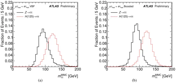
The MMC algorithm provides a solution for ∼99% of the H → ττ and Z → ττ events. This is a distinct advantage compared to the mass calculation using the colinear approximation where the failure rate is higher due to the implicit colinearity assumptions. The small loss rate of about 1% for signal events is due to large fluctuations of the E

measurement or other scan variables. In Figure 1 reconstructed m

mass distributions are shown for τ

τ

signal events with a mass of 125 GeV in the VBF and Boosted categories. The mass resolution, R , is found to be 15% and 16% for the VBF and Boosted categories respectively. The resolutions in the other categories are: R

lepτlep

≈ 16%, R

lepτlep

≈ 16%, R

hadτhad

≈ 14%, and R

hadτhad

≈ 14%. The distributions of reconstructed m

for Z → ττ background events are also shown in Figure 1.

[GeV]

τ τ

mMMC

0 50 100 150 200

Fraction of Events / 5 GeV

0 0.02 0.04 0.06 0.08 0.1 0.12 0.14 0.16 0.18 0.2 0.22

τ τ Z→

τ τ (125)→ H

ATLAS Preliminary

had VBF eτ

had + τ µ

(a)

[GeV]

τ τ

mMMC

0 50 100 150 200

Fraction of Events / 5 GeV

0 0.02 0.04 0.06 0.08 0.1 0.12 0.14 0.16 0.18 0.2 0.22

τ τ Z→

τ τ (125)→ H

ATLAS Preliminary Boosted

τhad

+ e τhad

µ

(b)

Figure 1: The reconstructed m

mass distributions for H → ττ (m

= 125 GeV) and Z → ττ events

in MC simulation and embedding, respectively, for events passing the VBF selection (a) and the Boosted

(b) selection in the τ

τ

channel.

5 Boosted decision trees

Boosted decision trees are used in each category to extract the Higgs boson signal from the large num- ber of background events. Decision trees [22] recursively partition the parameter space into multiple regions where signal or background purities are enhanced. Boosting is a method which improves the performance and stability of decision trees and involves the combination of many trees into a single final discriminant [23, 24]. After boosting, the final score undergoes a transformation to map the scores on the interval −1 to 1. The most signal-like events have scores near 1 while the most background-like events have scores near − 1.

Separate BDTs are trained for each analysis category and channel with signal and background sam- ples, described in Section 6, at √

s = 8 TeV. They are then applied to the analysis of the data of both centre-of-mass energies. The separate training naturally exploits differences in event kinematics between di ff erent Higgs boson production modes. It also allows di ff erent discriminating variables to be used to address the different background compositions in each channel. For the training in the VBF category only a VBF signal sample is used, while in the Boosted category gluon fusion, VBF, and V H signal samples are included. The Higgs boson mass has been chosen to be m

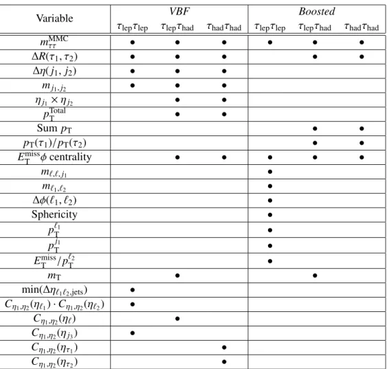
= 125 GeV for all signal samples. The BDT input variables used at both centre-of-mass energies are listed in Table 5. Most of these variables have straightforward definitions, and the more complex ones are defined in the following:

• ∆ R(τ

, τ

): The distance in ∆ R between the two leptons, between the lepton and τ

, or between the two τ

candidates, depending on the decay mode.

• p

: magnitude of the vector sum of the visible components of the tau decay products, the two leading jets, and E

.

• Sum p

: scalar sum of the p

of the visible components of the tau decay products and of the jets.

• E

φ centrality: a variable that quantifies the relative angular position of the missing transverse momentum with respect to the tau decay products in the transverse plane. The transverse plane is transformed such that the direction of the tau decay products are orthogonal, and that the smaller φ angle between the tau decay products defines the positive quadrant of the transformed plane.

E

φ centrality is defined as the sum of the x and y components of the E

unit vector in this transformed plane.

• Sphericity: a variable that describes the isotropy of the energy flow in the event [100]. It is based on the quadratic momentum tensor

S

= P

i

p

p

P

i

| p ~

| . (1)

In this equation, α and β are the indices of the tensor. The summation is performed over the momenta of the selected leptons and jets in the event. The sphericity of the event (S ) is then defined in terms of the two smallest eigenvalues of this tensor, λ

and λ

:

S = 3

2 (λ

+ λ

). (2)

• Object η centrality: a variable that quantifies the η position of an object (an isolated lepton, a τ

candidate or a jet) with respect to the two leading jets in the event. It is defined as

C

(η) = exp

"

−4 (η

− η

)

η − η

+ η

2

#

, (3)

where η, η

and η

are the pseudorapidities of the object and the two leading jets respectively. This variable has a value of 1 when the object is halfway in η between the two jets, 1/e when the object is aligned with one of the jets, and < 1/e when the object is outside the jets. In the τ

τ

channel the η centrality of a third jet in the event, C

(η

), and the product of the η centralities of the two leptons are used as BDT input variables, while in the τ

τ

channel the η centrality of the lepton, C

(η

), is used, and in the τ

τ

channel the η centrality of each τ, C

(η

) and C

(η

), is used. Events with only two jets are assigned a dummy value of −0.5 for C

(η

).

Among these variables, the most discriminating ones include: m

, ∆ R(τ

, τ

) and ∆ η( j

, j

).

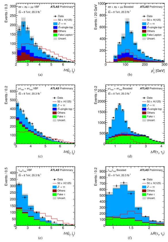
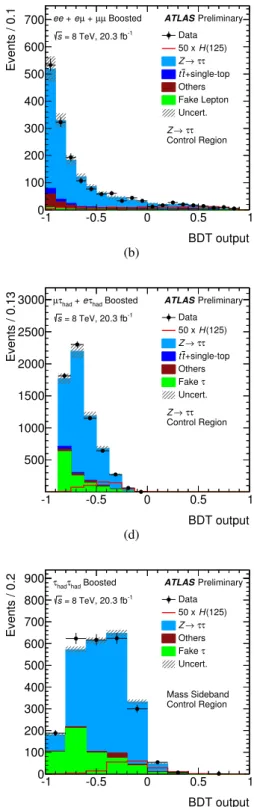
In Figure 2 the distributions of selected BDT input variables are shown. For the VBF category, the distributions of ∆ η( j

, j

) are shown for all three channels. For the Boosted category the distributions of

∆ R(τ

, τ

) are shown for the τ

τ

and τ

τ

channels and the distribution of the p

of the leading jet is shown for the τ

τ

channel. For all distributions the data are compared to the predictions from SM background processes at √

s = 8 TeV. The corresponding uncertainties are indicated by the shaded bands. All input distributions are well described, giving confidence that the background models (from simulation and data) describe well the relevant input variables of the BDT. Similarly good agreement is found for the distributions at √

s = 7 TeV.

Variable VBF Boosted

τ

τ

τ

τ

τ

τ

τ

τ

τ

τ

τ

τ

m

• • • • • •

∆ R(τ

, τ

) • • • • •

∆ η( j

, j

) • • •

m

• • •

η

× η

• •

p

• •

Sum p

• •

p

(τ

)/ p

(τ

) • •

E

φ centrality • • • • •

m

•

m

•

∆ φ(`

, `

) •

Sphericity •

p

•

p

•

E

/ p

•

m

• •

min(∆ η

) • C

(η

) · C

(η

) •

C

(η

) •

C

(η

) •

C

(η

) •

C

(η

) •

Table 5: Discriminating variables used in the training of the BDT for each channel and category at

√ s = 8 TeV. The filled circles indicate which variables are used in each case. Variables such as

∆ R(τ

, τ

) are defined between the two leptons, between the lepton and τ

, or between the two τ

candidates, depending on the decay mode.

2)

1, j (j η

∆

2 3 4 5 6 7

Events / 0.3

50 100 150 200 250 300

Data (125) 50 x H

τ τ

→ Z

+single-top t t Others Fake Lepton Uncert.

VBF µ + µ eµ +

ee ATLASPreliminary

, 20.3 fb-1 = 8 TeV s

(a)

[GeV]

j1

pT

0 100 200 300

Events / 20 GeV

200 400 600 800 1000

Data (125) H 50 x

τ τ Z→

+single-top t t Others Fake Lepton Uncert.

Boosted µ + µ eµ +

ee ATLASPreliminary

, 20.3 fb-1 = 8 TeV s

(b)

2)

1, j (j η

∆

3 4 5 6 7

Events / 0.2

0 100 200 300 400 500 600

Data (125) 50 x H

τ τ

→ Z

+single-top t t Others Fake τ Uncert.

had VBF τ + e τhad

µ ATLASPreliminary

, 20.3 fb-1 = 8 TeV s

(c)

2) , τ τ1

(

∆R

1 2 3 4

Events / 0.2

0 500 1000 1500 2000 2500

Data (125) 50 x H

τ τ

→ Z

+single-top t t Others Fake τ Uncert.

Boosted τhad

+ e τhad

µ ATLASPreliminary

, 20.3 fb-1 = 8 TeV s

(d)

2)

1, j (j η

∆

2 3 4 5 6 7

Events / 0.5

0 50 100 150 200 250 300 350 400

Data (125) 50 x H

τ τ

→ Z Others Fake τ Uncert.

had VBF

hadτ

τ ATLASPreliminary

, 20.3 fb-1 = 8 TeV s

(e)

2) , τ τ1

(

∆R

1 1.5 2

Events / 0.2

0 100 200 300 400 500 600 700 800 900

Data (125) 50 x H

τ τ Z→ Others Fake τ Uncert.

Boosted τhad

τhad ATLASPreliminary , 20.3 fb-1

= 8 TeV s

(f)

Figure 2: Distributions of important BDT input variables for the three channels and the two categories (VBF, left) and (Boosted, right) for data collected at √

s = 8 TeV. The distributions are shown for (a)

∆ η( j

, j

) and (b) p

( j

) in the τ

τ

channel, for (c) ∆ η( j

, j

) and (d) ∆ R(τ

, τ

) in the τ

τ

channel and for (e) ∆ η( j

, j

) and (f) ∆ R(τ

, τ

) in the τ

τ

channel. The contributions from a

Standard Model Higgs boson with m

= 125 GeV are superimposed, multiplied by a factor of 50. These

figures use background predictions made without the global fit defined in Section 8. The error band

includes statistical and pre-fit systematic uncertainties.

6 Background estimation

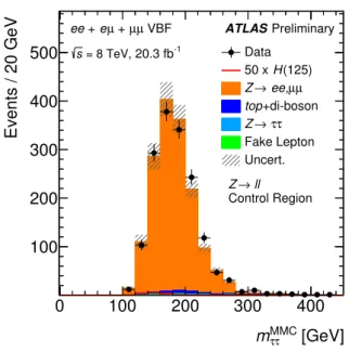
The di ff erent final-state topologies of the three analysis channels have di ff erent background compositions which necessitate different strategies for the background estimation. In general, the number of expected background events and the associated kinematic distributions are derived from a mixture of data-driven methods and simulation. The normalisation of several important background contributions is performed by comparing the simulated samples of individual background sources to data in regions which only have a small or negligible contamination from signal or other background events.

Common to all channels is the dominant Z → ττ background, for which the kinematic distributions are taken from data by employing the embedding technique, as described in Section 3. Background con- tributions from jets that are misidentified as hadronically decaying taus (fake backgrounds) are estimated by using either a fake factor method or samples of non-isolated τ

candidates. Likewise, samples of non-isolated leptons are used to estimate fake lepton contributions from either jets or hadronically decaying taus and leptons from other sources, such as heavy quark decay.

Other non-fake contributions from various physics processes are estimated using the simulation, normalised to the theoretical cross sections, as given in Table 1. A more detailed discussion on the estimation of the various background components in the different channels is given in the following.

6.1 Backgrounds from Z → ττ production

A reliable modelling of the irreducible Z → ττ background is an important ingredient of the analysis.

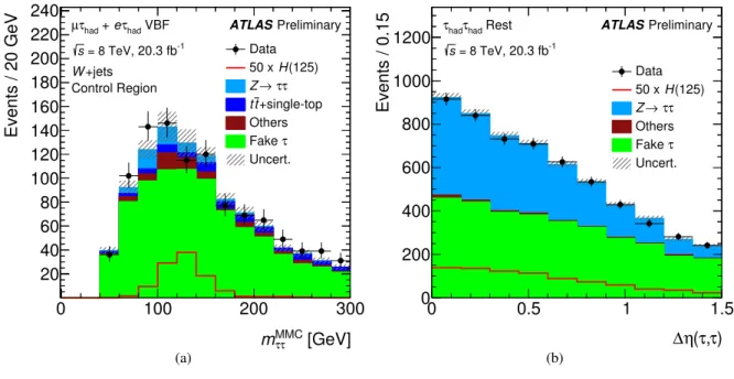
Since it is not possible to select a su ffi ciently pure and signal-free Z → ττ control sample from data, the contribution of this background is estimated using embedded data. This procedure has been extensively validated by using both data and simulation. To validate the subtraction procedure of the muon cell energies and tracks from data and the subsequent embedding of the corresponding information from simulation, the muons in Z → µµ events are replaced by simulated muons. The calorimeter isolation energy in a cone of ∆ R = 0.3 around the muons from data before and after embedding are compared in Figure 3(a). Good agreement is found, which indicates that no deterioration in the muon environment is introduced. Another important test constitutes the validation of the embedding of more complex Z → ττ events, which can only be performed in the simulation. To achieve a meaningful validation, the same MC generator with identical settings was used to simulate both Z → µµ and Z → ττ events. The sample of embedded events is corrected for the bias due to the trigger, reconstruction and acceptance of the original muons. These corrections are determined from data as a function of p

(µ) and η(µ), and allow the acceptance of the original selection to be corrected. The tau decay product are treated as any other objects determined from the simulation, with one important di ff erence due to the absence of trigger simulation in this sample. Trigger effects are parameterised from the simulation as a function of the tau decay product p

. After replacing the muons by simulated taus, kinematic distributions of the embedded sample can be directly compared to the simulated ones. As an example, the reconstructed invariant mass, m

, is shown in Figure 3(b). Also in this case, good agreement is found and the observed di ff erences are covered by the systematic uncertainties. Similarly, good agreement is found for other variables, such as the missing transverse energy, the kinematic variables of the hadronically decaying tau lepton or of the associated jets in the event. A direct comparison of the Z → ττ background in data and the modelling using the embedding technique also shows good agreement. This can be seen, e.g. from several distributions of kinematic quantities, which are dominated by Z → ττ events, shown in Figure 2.

The normalisation for this background process is taken from the final fit described in Section 8. The normalisation is taken to be independent for the τ

τ

, τ

τ

, and τ

τ

analysis channels.

8Leptons from heavy quark decays are considered as fake leptons in the following.

) [GeV]

( µ p

, 0.3) ⋅ E

( I

Arbitrary Units

0 0.05 0.1 0.15 0.2 0.25 0.3 0.35

Data

Embedded Data ATLASPreliminary µ

µ Z→

) [GeV]

( µ p

, 0.3) ⋅ E

I (

0 2 4 6 8 10

Emb. / Data

0.8 0.9 1 1.1 1.2

(a)

MMC [GeV]

60 80 100 120 140 160 180

Arbitrary Units

0 0.02 0.04 0.06 0.08 0.1 0.12 0.14 0.16

MC

MC Stat. Error Embedded MC Emb. Uncertainty ATLASSimulation

Preliminary

[GeV]

MMC τ

m

60 80 100 120 140 160 180

Emb. / MC

0.8 0.9 1 1.1 1.2

(b)

Figure 3: (a) The distribution of the calorimeter isolation energy I(E

, 0.3) · p

(µ) within a cone of

radius ∆ R = 0.3 around the muons in Z → µµ events from data, before and after embedding of simulated

muons. (b) The distribution of the reconstructed invariant ττ mass, m

, for simulated Z → ττ events,

compared to the one obtained from simulated Z → µµ events after tau embedding. The ratios of the

values before and after embedding and between the embedded Z → µµ and Z → ττ events are given in (a)

and (b) respectively. The errors in (a) and (b) on the ratios (points) represent the statistical uncertainties,

while the systematic uncertainties are indicated by the hatched bands in (b). The shaded bands represent

the statistical uncertainties from the Z → µµ data event in (a) and from the Z → ττ MC in (b).

6.2 Backgrounds from misidentified leptons or hadronically decaying taus

For the τ

τ

channel, all background sources resulting from misidentified leptons are treated together.

In this approach contributions from multijet and W + jets production, as well as the part of the t¯ t back- ground resulting from lepton-hadron decays (t¯ t → `νb qqb) are included. A control sample is defined in data by inverting the isolation selections for one of the two leptons, while applying all other signal region requirements. The contributions from other background channels (dileptonic t¯ t decays (t¯ t → `νb `νb), Z → ee, Z → µµ, and diboson production) are obtained from the simulation and are subtracted. From this control sample a template is created. The normalisation factor is obtained by fitting the p

distribution of the sub-leading lepton at an early stage of the pre-selection.

For the τ

τ

channel, the fake-factor method is used to derive estimates for the multijet, W + jets, Z + jets, and semi-leptonic t¯ t background events that pass the τ

τ

selection due to a misidentified τ

candidate. The fake factor is defined as the ratio of the number of τ

candidates identified as medium, to the number passing the loose, but not the medium criteria. Since the fake factor depends on the nature and on the p

of the jet, it is determined as a function of p

separately for quark- and gluon-enriched samples. In addition, the fake factor is found to be different for 1-track and 3-track candidates. Three di ff erent, quark-jet dominated samples are used separately for the W + jets, t¯ t and Z + jets background components. They are defined by selecting the high-m

region (m

> 70 GeV), by inverting the b-tag veto and by requiring two leptons with an invariant mass consistent with m

(80 GeV < m

< 100 GeV) respectively. In addition, a gluon-jet dominated multijet sample is selected by relaxing the lepton identification and requiring the lepton to pass the loose identification criteria.

The derived fake factors are found to vary from 0.124 (0.082) for p

= 20 GeV to 0.088 (0.038) for p

= 150 GeV for 1-track (3-track) candidates in the VBF category. The corresponding values for the Boosted category are 0.146 (0.084) for p

= 20 GeV and 0.057 (0.033) for p

= 150 GeV. To obtain the fake background estimate for the VBF and Boosted signal regions, these factors are then applied, weighted by the expected relative W +jets, Z +jets, multijet, and t¯ t fractions, to the events in regions defined by applying the selections of the corresponding signal region, except that the τ

candidate is required to pass the loose and to fail the medium τ

identification. As an example, the good agreement between data and background estimations is shown in Figure 4(a) for the reconstructed ττ mass for events in the high-m

region, which is dominated by fakes from W + jets production.

For the τ

τ

channel, the multijet background is modelled using a template extracted from data that pass the VBF or Boosted signal selection, where, however, the taus fail the isolation and opposite-sign charge requirements. The normalisation of the multijet background is first determined by performing a simultaneous fit of the multijet (modelled by the data sample just mentioned) and Z → ττ (modelled by embedding) templates after the pre-selection cuts. The fit is performed for the distribution of the differ- ence in pseudorapidity between the two hadronic tau candidates, ∆ η(τ

, τ

). The signal contribution is expected to be small in this category. The agreement between data and background estimation for this distribution is shown in Figure 4(b) for a control region using the Rest category defined in Section 4. The preselection normalisation is used as a reference point and starting value for the global fit (see below) and is used for validation plots. The final normalisations of the two important background components, from multijet and Z → ττ events, are extracted from the final global fit, as described in Section 8, in which the ∆ η(τ

, τ

) distribution for the Rest category is included.

6.3 Z → ee and Z → µµ backgrounds

The Drell-Yan Z/γ

→ ee and Z/γ

→ µµ background channels are important for the final states with

two same-flavour leptons. They also contribute to the other channels. As described below, a simulation

based on Alpgen has been used to estimate these background sources. Correction factors are applied to

account for differences between data and simulation.