Combined coupling measurements of the Higgs-like boson with the ATLAS detector using up to 25 fb

ATLAS-CONF-2013-034 14March2013

ATLAS NOTE

ATLAS-CONF-2013-034

March 13, 2013

Combined coupling measurements of the Higgs-like boson with the ATLAS detector using up to 25 fb

of proton-proton collision data

The ATLAS Collaboration

Abstract

This note presents an update of the measurements of the properties of the newly dis- covered boson using the full

collision data sample recorded by the ATLAS experi- ment at the LHC for the channels

4` and

responding to integrated luminosities of up to 4.8 fb

at

s =

7 TeV and 20.7 fb

at

√s=

8 TeV. The combination also includes results from the

and

¯ channels based on

collision data corresponding to an integrated luminosity of up to 4.7 fb

at

√s =

7 TeV and 13 fb

at

s =

8 TeV. The combined signal strength is determined to be

1

30

0

13 (stat)

0

14 (sys) at a mass of 125.5 GeV. The cross section ratio be- tween vector boson mediated and gluon (top) initiated Higgs boson production processes is found to be

1.2

, giving more than 3σ evidence for Higgs-like boson production through vector-boson fusion. Measurements of relative branching fraction ratios between the

,

4

and

channels, as well as combined fits testing the fermion and vector coupling sector, couplings to

and

and loop induced processes of the Higgs-like boson show no significant deviation from the Standard Model expectation.

c Copyright 2013 CERN for the benefit of the ATLAS Collaboration.

Reproduction of this article or parts of it is allowed as specified in the CC-BY-3.0 license.

1 Introduction

The observation of a new particle in the search for the Standard Model (SM) Higgs boson at the LHC, reported by the ATLAS [1] and CMS [2] Collaborations, is a milestone in the quest to understand elec- troweak symmetry breaking. In Refs. [1] and [3] the ATLAS Collaboration reported first measurements of the mass of the particle and its coupling properties. The combined signal strength value for the chan- nels H → WW

→ `ν`ν , H → ττ and H → b b ¯ was reported in Ref. [4]. The mass and signal strength measurements were updated in Refs. [5, 6] based on 13 fb

of data at √

s

8 TeV and 20.7 fb

at

√ s

8 TeV respectively for the high mass resolution channels.

This document presents an update of the measurements of signal strength and couplings of the ob- served new particle using 4.8 fb

of pp collision data at √

s

7 TeV and 20.7 fb

at √

s

8 TeV for the three most sensitive channels H → γγ [7], H → ZZ

→ 4 ` [8] and H → WW

→ `ν`ν [9].

The results are based on the same statistical model as in Refs. [1, 3]. The aspects of the individual channels relevant for these measurements are briefly summarized in Section 2. The statistical proce- dure and the treatment of systematic uncertainties are outlined in Section 3. In Section 4 the measured yields are analysed in terms of the signal strengths, for di

erent production and decays modes, and their combinations.

Finally, in Section 5 the couplings of the newly discovered boson are tested through fits to the ob- served data. These studies aim to probe, under the assumptions described in the text, the Lagrangian structure in the vector boson and fermion sectors, the ratio of couplings to the W and Z bosons and the loop induced couplings to gluons and photons.

2 Input Channels

For the H→ γγ, H → ZZ

and H → WW

channels, the updated analyses based on the full 2011 and 2012 datasets as presented in Refs. [7–9] are used. For the H → ττ and H → b b ¯ channels, the analyses [10, 11] are applied to the full 2011 data sample at √

s

7 TeV and a subsample of the 2012 data corresponding to 13 fb

at √

s

8 TeV . The different final states and channel categories considered in this analysis are summarized in Table 1.

3 Statistical Procedure

The statistical modelling of the data is described in Refs. [12–16]. Systematic uncertainties on observ- ables are handled by introducing nuisance parameters. When these parameters are related to observables that are estimated externally an additional constraint is added to the model as a probability density func- tion (pdf) associated with the uncertainty on the corresponding parameter. The typical constraints used are Gaussian, log-normal or gamma distributions. Rectangular pdfs are also used in specific cases which will be detailed in this note. The latter give a flat a priori likelihood in the range of the ±1σ Gaussian uncertainty intervals for the corresponding sources of systematic uncertainties. The use of such a pdf model for systematic uncertainties could lead to a coherent shift of the nuisance parameters within their allowed range to values which reduce the tension between measurements.

The number of signal events in the likelihood function is parametrized in terms of scale factors for

the cross section σ

of each SM Higgs boson production mode i, the branching ratios B

of the SM

Higgs boson decay modes f , and the mass of the Higgs boson m

. For each production mode, a signal

strength factor µ

σ

/σ

is introduced. Similarly, for each decay final state, a factor µ

B

/ B

is introduced. For each analysis category (k) the number of signal events (n

) is parametrized as:

n



∑

i

µ

σ

× A

× ε





× µ

× B

× L

(1)

where A represents the detector acceptance, ε the reconstruction efficiency and L the integrated lumi- nosity. The number of signal events expected from each combination of production and decay mode is scaled by the corresponding product µ

µ

, with no change to the distribution of kinematic or other properties. This parametrization generalizes the dependence of the signal yields on the production cross sections and decay branching fractions, allowing for a coherent variation across several channels. This approach is also general in the sense that it is not restricted by any relationship between production cross sections and branching ratios. The relationship between production and decay in the context of a specific theory or benchmark is achieved via a parametrization of µ

, µ

→ f (

), where

are the parameters of

Table 1: Summary of the individual channels entering the combined results presented here. In channels sensitive to associated production of the Higgs boson, V indicates a W or Z boson. The symbols ⊗ and ⊕ represent direct products and sums over sets of selection requirements, respectively. The abbreviations listed here are described in the corresponding References indicated in the last column. For the determi- nation of the combined signal strength µ , reported in Section 4, the inclusive H → ZZ

→ 4 ` analysis [8]

is used.

Higgs Boson Subsequent

Sub-Channels

∫

L dt

Decay Decay [fb

] Ref.

2011 √

s

7 TeV

H → ZZ

4` {4e, 2e2µ, 2µ2e, 4µ, 2-jet VBF, `-tag} 4.6 [8]

H → γγ – 10 categories

4.8 [7]

{ p

⊗ η

⊗ conversion } ⊕ { 2-jet VBF }

H → WW

`ν`ν { ee , e µ, µ e , µµ} ⊗ { 0-jet, 1-jet, 2-jet VBF } 4.6 [9]

H → ττ

τ

τ

{ e µ} ⊗ { 0-jet } ⊕ {``} ⊗ { 1-jet, 2-jet, p

> 100 GeV, V H } 4.6

τ

τ

{ e , µ} ⊗ { 0-jet, 1-jet, p

> 100 GeV, 2-jet } 4.6 [10]

τ

τ

{1-jet, 2-jet} 4.6

V H → Vbb

Z → νν E

∈ {120 − 160, 160 − 200, ≥ 200 GeV} ⊗ {2-jet, 3-jet} 4.6

W → `ν p

∈ {< 50, 50 − 100, 100 − 150, 150 − 200, ≥ 200 GeV} 4.7 [11]

Z → `` p

∈ {< 50 , 50 − 100 , 100 − 150 , 150 − 200 , ≥ 200 GeV } 4.7 2012 √

s

8 TeV

H → ZZ

4 ` { 4e , 2e2 µ, 2 µ 2e , 4 µ, 2-jet VBF , ` -tag }} 20.7 [8]

H → γγ – 14 categories

20.7 [7]

{ p

⊗ η

⊗ conversion } ⊕ { 2-jet VBF } ⊕ {` -tag, E

-tag, 2-jet VH }

H → WW

`ν`ν { ee , e µ, µ e , µµ} ⊗ { 0-jet, 1-jet, 2-jet VBF } 20.7 [9]

H → ττ

τ

τ

{``} ⊗ { 1-jet, 2-jet, p

> 100 GeV, V H } 13

τ

τ

{e, µ} ⊗ {0-jet, 1-jet, p

> 100 GeV, 2-jet} 13 [10]

τ

τ

{ 1-jet, 2-jet } 13

V H → Vbb

Z → νν E

∈ {120 − 160, 160 − 200, ≥ 200 GeV} ⊗ {2-jet, 3-jet} 13

W → `ν p

∈ {< 50 , 50 − 100 , 100 − 150 , 150 − 200 , ≥ 200 GeV } 13 [11]

Z → `` p

∈ {< 50 , 50 − 100 , 100 − 150 , 150 − 200 , ≥ 200 GeV } 13

the theory or benchmark under consideration as defined in Section 5. In the simplest cases the product µ

µ

is also represented by a single signal strength parameter µ

, where j is an index representing both the production and decay indices i and f . For example, the global signal strength µ scales the total num- ber of events from all combinations of production and decay modes relative to their SM values, such that µ

0 corresponds to the background-only hypothesis and µ

1 corresponds to the SM Higgs boson signal in addition to the background.

The likelihood is a function of a vector of signal strength factors

m

and the nuisance parameters

. Hypothesis testing and confidence intervals are based on the profile likelihood ratio [17].

The parameters of interest are di

erent in the various tests, while the remaining parameters are profiled.

Hypothesized values of

are tested with a statistic

(

)

L

ˆˆ (

)

L( ˆ

ˆ ) , (2)

where the single circumflex denotes the unconditional maximum likelihood estimate of a parameter and the double circumflex (e.g.

ˆˆ (

)) denotes the conditional maximum likelihood estimate (e.g. of

) for given fixed values of

. This test statistic extracts the information on the parameters of interest from the full likelihood function. When the signal strength parameters

are reparametrized in terms of

same equation is used for

(

) with

→

.

Asymptotically, a test statistic − 2 ln

(

) of several parameters of interest

is distributed as a χ

distribution with n degrees of freedom, where n is the dimensionality of the vector

the 100(1 − α )% confidence level (CL) contours are defined by − 2 ln

(

) < k

, where k

satisfies P( χ

> k

)

α . For two degrees of freedom the 68% and 95% CL contours are given by − 2 ln

(

)

2 . 3 and 6.0, respectively. All contours shown in the following Sections are based on likelihood evaluations and can therefore be translated into CL contours only if the asymptotic approximation is valid.

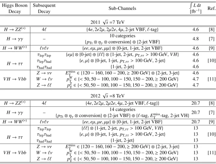
4 Signal Production Strength in Individual Decay Modes

This section focuses on the global signal strength parameter µ and the individual signal strength param- eters µ

which depend upon the production mode i and the decay mode f , for a fixed mass hypothesis m

. Hypothesized values of µ and µ

are tested with the statistic

The best-fit signal strength parameter µ is a convenient observable to test the compatibility of the data with the background-only hypothesis ( µ

0) and the SM Higgs hypothesis ( µ

1). The best- fit values of the signal strength parameter for each channel independently and for the combination are illustrated in Fig. 1 and in Table 2 for a mass of m

125 . 5 GeV, derived from the combination of the H → γγ and H → ZZ

→ 4 ` channels [6]. Checks allowing the Higgs boson mass hypothesis to float, using it as an additional nuisance parameter in measurements of

experimental uncertainty on its estimate, were performed and no significant deviations from the results presented herein were observed.

The measured global signal yield is ˆ µ

1.30 ± 0.13 (stat) ± 0.14 (sys) for m

125.5 GeV with all channels combined. This combined signal strength ˆ µ is consistent with the SM Higgs boson hypothesis µ

1 at the 9% level. The consistency with the SM Higgs boson hypothesis is also tested using rectan- gular pdfs for the dominant theory systematic uncertainties from gg → H QCD scale and PDF variations following the recommendations in Refs. [19, 20]. With this treatment, the consistency of the observed signal strength with the SM hypothesis increases to ∼ 40%. The global compatibilty between the signal

1HereΛis used for the profile likelihood ratio to avoid confusion with the parameterλused in Higgs boson coupling scale factor benchmarks [18].

2Whenever probabilities are translated into number of Gaussian standard deviations the two-sided convention is chosen.

strengths of the five channels and the SM expectation of one is about 8%. The compatibility between the combined best-fit signal strength ˆ µ and the best-fit signal strengths of the five channels is 13%. The dependence of the combined value of ˆ µ on the assumed m

has been investigated and is relatively weak:

changing the mass hypothesis between 124.5 and 126.5 GeV changes the value of ˆ µ by about 4%.

Table 2: Summary of the best-fit values and uncertainties for the signal strength µ for the individual channels and their combination at a Higgs boson mass of 125.5 GeV.

Higgs Boson Decay µ

(m

125.5 GeV) V H → Vbb − 0 . 4 ± 1 . 0

H → ττ 0 . 8 ± 0 . 7 H → WW

1 . 0 ± 0 . 3 H → γγ 1 . 6 ± 0 . 3 H → ZZ

1 . 5 ± 0 . 4 Combined 1 . 30 ± 0 . 20

µ ) Signal strength ( -1 0 +1

Combined

→ 4l ZZ(*)

→ H

γ γ

→ H

ν νl

→ l WW(*)

→ H

τ τ

→ H

→ bb W,Z H

Ldt = 4.6 - 4.8 fb-1

∫

= 7 TeV:

s

Ldt = 13 - 20.7 fb-1

∫

= 8 TeV:

s

Ldt = 4.6 fb-1

∫

= 7 TeV:

s

Ldt = 20.7 fb-1

∫

= 8 TeV:

s

Ldt = 4.8 fb-1

∫

= 7 TeV:

s

Ldt = 20.7 fb-1

∫

= 8 TeV:

s

Ldt = 4.6 fb-1

∫

= 7 TeV:

s

Ldt = 20.7 fb-1

∫

= 8 TeV:

s

Ldt = 4.6 fb-1

∫

= 7 TeV:

s

Ldt = 13 fb-1

∫

= 8 TeV:

s

Ldt = 4.7 fb-1

∫

= 7 TeV:

s

Ldt = 13 fb-1

∫

= 8 TeV:

s

= 125.5 GeV mH

0.20

± = 1.30 µ

ATLAS Preliminary

Figure 1: Measurements of the signal strength parameter µ for m

125.5 GeV for the individual chan- nels and their combination.

In the SM, the production cross sections are completely fixed once m

is specified. The best-fit value

for the global signal strength factor µ does not give any direct information on the relative contributions

from di

erent production modes. Furthermore, fixing the ratios of the production cross sections to the

ratios predicted by the SM may conceal tension between the data and the SM. Therefore, in addition to

the signal strength in different decay modes, the signal strengths of different Higgs production processes

contributing to the same final state are determined. Such a separation avoids model assumptions needed

for a consistent parametrization of both production and decay modes in terms of Higgs boson couplings.

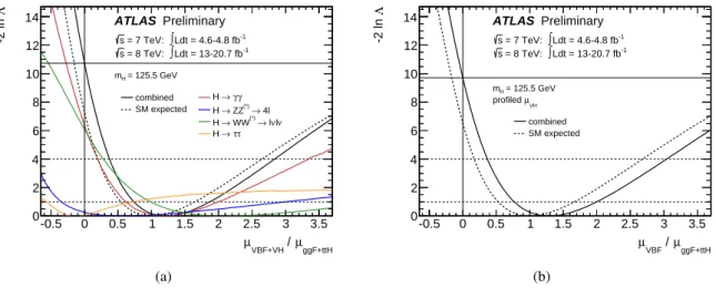
Since several Higgs boson production modes are available at the LHC, results shown in two di- mensional plots require either some µ

to be fixed or several µ

to be related. No direct t¯ tH production has been observed yet, hence a common signal strength scale factor µ

has been assigned to both gluon fusion production (ggF) and the very small t tH ¯ production mode, as they both scale dominantly with the ttH coupling in the SM. Similarly, a common signal strength scale factor µ

has been assigned to the VBF and V H production modes, as they scale with the W H/ZH gauge coupling in the SM. The resulting contours for the H → γγ , H → WW

→ `ν`ν , H → ZZ

→ 4 ` and H → ττ channels for m

125.5 GeV are shown in Fig. 2.

B/B

×

µ

-2 -1 0 1 2 3 4 5 6 7 8

SM

B/B ×

µ

-4 -2 0 2 4 6 8 10

Standard Model Best fit 68% CL 95% CL γ

γ

→ H

→ 4l ZZ(*)

→ H

ν νl

→ l WW(*)

→ H

τ τ

→ H

Preliminary ATLAS

Ldt = 4.6-4.8 fb-1

∫

= 7 TeV:

s

Ldt = 13-20.7 fb-1

∫

= 8 TeV:

s

= 125.5 GeV mH

Figure 2: Likelihood contours for the H→ γγ, H→ ZZ

→ 4`, H→ WW

→ `ν`ν and H → ττ channels in the ( µ

, µ

) plane for a Higgs boson mass hypothesis of m

125 . 5 GeV. Both µ

and µ

are modified by the branching ratio factors B / B

, which are di

erent for the di

erent final states. The quantity µ

(µ

) is a common scale factor for the gluon fusion and t tH ¯ (VBF and V H ) production cross sections. The best fit to the data ( × ) and 68% (full) and 95% (dashed) CL contours are also indicated, as well as the SM expectation (

).

The factors µ

are not constrained to be positive in order to account for a deficit of events from the corresponding production process. As described in Ref. [12], while the signal strengths may be negative, the total probability density function must remain positive everywhere, and hence the total number of expected signal+background events has to be positive everywhere. This restriction is responsible for the sharp cuto

in the H → ZZ

→ 4 ` contour. It should be noted that each contour refers to a di

erent branching fraction B / B

, hence a direct combination of the contours from di

erent final states is not possible.

It is nevertheless possible to use the ratio of production modes channel by channel to eliminate the

dependence on the branching fractions and illustrate the relative discriminating power between ggF

t¯ tH

and VBF

V H, and test the compatibility of the measurements among channels. The relevant channels

have the following proportionality:

σ(gg → H) ∗ BR(H→ γγ) ∼ µ

σ (qq

→ qq

H) ∗ BR(H → γγ ) ∼ µ

· µ

/µ

σ ( gg → H) ∗ BR(H → ZZ

) ∼ µ

σ (qq

→ qq

H) ∗ BR(H → ZZ

) ∼ µ

· µ

/µ

σ ( gg → H) ∗ BR(H → WW

) ∼ µ

(3) σ (qq

→ qq

H) ∗ BR(H → WW

) ∼ µ

· µ

/µ

σ ( gg → H) ∗ BR(H → ττ ) ∼ µ

σ(qq

→ qq

H) ∗ BR(H → ττ) ∼ µ

· µ

/µ

where µ

is defined as

µ

σ (ggF) · BR(H → XX)

σ

(ggF) · BR

(H → XX)

σ (t¯ tH) · BR(H → XX)

σ

(t tH) ¯ · BR

(H → XX) (4) and µ

/µ

is the parameter of interest giving the ratio between VBF

V H and ggF

t tH ¯ scale factors.

The likelihood as a function of the common ratio µ

/µ

, while profiling over all pa- rameters µ

, is shown in Fig. 3 for the H→ γγ, H→ ZZ

→ 4`, H→ WW

→ `ν`ν and H → ττ channels and their combination. For this combination it is only necessary to assume that the same boson H is responsible for all observed Higgs-like signals and that the separation of gluon- fusion-like events and VBF-like events within the individual analyses based on the event kinematic properties is valid. The measurements in the four channels, as well as the observed combined ratio µ

/µ

1 . 2

, are compatible with the SM expectation of unity. The p-value

when test- ing the hypothesis µ

/µ

0 is 0.05% , corresponding to a significance against the vanishing vector boson mediated production assumption of 3.3σ. The ratio µ

/µ

, where the signal strength µ

of the V H Higgs production process is profiled instead of being treated together with µ

, gives the same result of µ

/µ

1 . 2

. The p-value for µ

/µ

0 is 0.09% corresponding to a significance against the vanishing VBF production assumption of 3.1σ.

In another approach the dependence on the individual production µ

cancels out when taking the ratio of µ

× BR within the same production mode. For the example of the H → γγ and H → ZZ

→ 4 ` channels, this results in a ratio of relative branching ratios ρ, defined as:

ρ

BR(H → γγ )

BR(H → ZZ

) × BR

(H → ZZ

)

BR

(H → γγ ) , (5)

where the first term is the ratio of branching ratios and the second term rescales this ratio to the SM expectations. The relevant channels have the following proportionality:

σ ( gg → H) ∗ BR(H → γγ ) ∼ µ

· ρ

σ(qq

→ qq

H) ∗ BR(H→ γγ) ∼ µ

· µ

/µ

· ρ

σ ( gg → H) ∗ BR(H → ZZ

) ∼ µ

(6)

σ (qq

→ qq

H) ∗ BR(H → ZZ

) ∼ µ

· µ

/µ

3The p-value and significance are calculated for the test hypothesisµVBF+V H/µggF+t¯tH =0 against the one-sided alternative µVBF+V H/µggF+ttH¯ >0 using the profile likelihood test statistic.

ggF+ttH

µ

VBF+VH / µ

-0.5 0 0.5 1 1.5 2 2.5 3 3.5

Λ-2 ln

0 2 4 6 8 10 12 14

combined SM expected

γ γ

→ H

→ 4l ZZ(*)

→ H

ν νl

→ l WW(*)

→ H

τ τ

→ H

Preliminary ATLAS

Ldt = 4.6-4.8 fb-1

∫

= 7 TeV:

s

Ldt = 13-20.7 fb-1

∫

= 8 TeV:

s

= 125.5 GeV mH

(a)

ggF+ttH

µ

VBF / µ

-0.5 0 0.5 1 1.5 2 2.5 3 3.5

Λ-2 ln

0 2 4 6 8 10 12 14

combined SM expected

Preliminary ATLAS

Ldt = 4.6-4.8 fb-1

∫

= 7 TeV:

s

Ldt = 13-20.7 fb-1

∫

= 8 TeV:

s

= 125.5 GeV mH

µVH profiled

(b)

Figure 3: Likelihood curves for the ratio (a) µ

/µ

and (b) µ

/µ

for the H → γγ , H → ZZ

→ 4 ` , H → WW

→ `ν`ν and H → ττ channels and their combination for a Higgs boson mass hypothesis of m

125.5 GeV. The branching ratios and possible non-SM effects coming from the branching ratios cancel in µ

/µ

and µ

/µ

, hence the di

erent measurements from all four channels can be compared and combined. For the measurement of µ

/µ

, the signal strength µ

is profiled. The dashed curves show the SM expectation for the combination. The horizontal dashed lines indicate the 68% and 95% confidence levels.

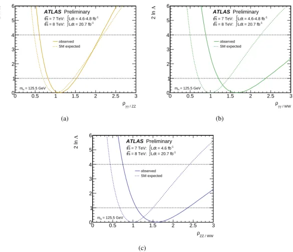
Figure 4 shows the likelihood as a function of the ratios ρ

for pairwise combinations of the H→ γγ, H→ ZZ

→ 4` and H→ WW

→ `ν`ν channels, while profiling over the parameters µ

and µ

/µ

. The best-fit values are

ρ

1 . 1

ρ

1.7

(7)

ρ

1.6

, in agreement with the SM expectation of one.

5 Coupling fits

In the previous section signal strength scale factors µ

for either the Higgs production or decay modes were determined. However, for a consistent measurement of Higgs boson couplings, production and de- cay modes cannot be treated independently. Following the framework and benchmarks as recommended in Ref. [18,21], measurements of coupling scale factors are implemented using a LO tree level motivated framework. This framework makes the following assumptions:

• The signals observed in the di

erent search channels originate from a single narrow resonance with a mass near 125.5 GeV. The case of several, possibly overlapping, resonances in this mass region is not considered.

• The width of the assumed Higgs boson near 125.5 GeV is neglected, i.e. the zero-width approxi- mation for this state is used. Hence the product σ × BR(ii → H →

) can be decomposed in the following way for all channels:

σ × BR(ii → H →

)

σ

·

ΓH

, (8)

/ ZZ γ

ργ

0 0.5 1 1.5 2 2.5 3

Λ2 ln

0 1 2 3 4 5 6

observed SM expected

Preliminary ATLAS

Ldt = 4.6-4.8 fb-1

∫ = 7 TeV:

s

Ldt = 20.7 fb-1

∫ = 8 TeV:

s

= 125.5 GeV mH

(a)

/ WW γ

ργ

0 0.5 1 1.5 2 2.5 3

Λ2 ln

0 1 2 3 4 5 6

observed SM expected

Preliminary ATLAS

Ldt = 4.6-4.8 fb-1

∫ = 7 TeV:

s

Ldt = 20.7 fb-1

∫ = 8 TeV:

s

= 125.5 GeV mH

(b)

ZZ / WW

ρ

0 0.5 1 1.5 2 2.5 3

Λ2 ln

0 1 2 3 4 5 6

observed SM expected

Preliminary ATLAS

Ldt = 4.6 fb-1

∫ = 7 TeV:

s

Ldt = 20.7 fb-1

∫ = 8 TeV:

s

= 125.5 GeV mH

(c)

Figure 4: Likelihood curves for pairwise ratios of branching ratios normalized to their SM expectations (a) ρ

, (b) ρ

and (c) ρ

of the H→ γγ, H→ ZZ

→ 4` and H→ WW

→ `ν`ν channels, for a Higgs boson mass hypothesis of m

125 . 5 GeV. The dashed curves show the SM expectation.

where σ

is the production cross section through the initial state ii,

the partial decay width into the final state

and

the total width of the Higgs boson.

• Only modifications of couplings strengths, i.e. of absolute values of couplings, are taken into ac- count, while the tensor structure of the couplings is assumed to be the same as in the SM prediction.

This means in particular that the observed state is assumed to be a CP-even scalar as in the SM.

The LO motivated coupling scale factors

are defined in such a way that the cross sections σ

and the partial decay widths

associated with the SM particle j scale with the factor

when compared to the corresponding SM prediction. Details can be found in Refs. [3, 18]

Taking the process gg → H →

as an example, one would write the cross section as:

σ · BR (gg → H →

)

σ

(gg → H) · BR

(H →

) ·

2g

·

κ²_H

(9)

where the values and uncertainties for both σ

(gg → H) and BR

(H →

) are taken from Refs. [19, 20, 22] for a given Higgs boson mass hypothesis.

In some of the fits the e

ective scale factors

and

for the processes H →

and gg → H, which

are loop induced in the SM, are treated as a function of the more fundamental coupling scale factors

,

κb

,

, and similarly for all other particles that contribute to these SM loop processes. In these cases the scaled fundamental couplings are propagted through the loop calculations, including all interference e

ects, using the functional form derived from the SM [21].

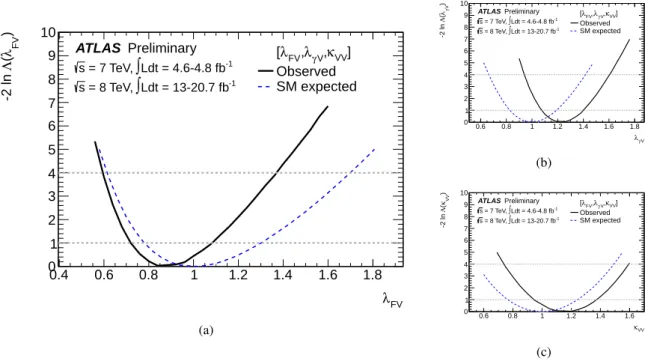
5.1 Fermion versus vector (gauge) couplings

This benchmark is an extension of the single parameter µ fit, where different strengths for the fermion and vector couplings are probed. It assumes that only SM particles contribute to the H → γγ and gg → H vertex loops, but any modification of the coupling strength factors for fermions and vector bosons are propagated through the loop calculations. The fit is performed in two variants, with and without the assumption that the total width of the Higgs boson is given by the sum of the known SM Higgs boson decay modes (modified in strength by the appropriate fermion and vector coupling scale factors).

5.1.1 Only SM contributions to the total width

The fit parameters are the coupling scale factors

for all fermions and

for all vector couplings:

κV = κW =κZ

(10)

κF = κt =κb=κτ =κg

(11)

As only SM particles are assumed to contribute to the gg → H vertex loop in this benchmark, the gluon fusion process measures directly the fermion scale factor

. For the most relevant Higgs boson production and decay modes the following proportionality is found:

σ(gg → H) ∗ BR(H→ γγ) ∼

2

F

·

(

,

) 0.75 ·

0.25 ·

σ(qq

→ qq

H) ∗ BR(H→ γγ) ∼

2

V

·

(

,

) 0.75 ·

0.25 ·

σ ( gg → H) ∗ BR(H → ZZ

, H → WW

) ∼

2 F

·

0 . 75 ·

0 . 25 ·

(12) σ (qq

→ qq

H) ∗ BR(H → ZZ

, H → WW

) ∼

2 V

·

0 . 75 ·

0 . 25 ·

σ (qq

→ qq

H , V H) ∗ BR(H → ττ, H → b b) ¯ ∼

2 V

·

0.75 ·

0.25 ·

,

where

(

,

) is the SM functional dependence of the effective scale factor

on the scale factors

and

, which is to first approximation:

κ²_γ

(

,

)

1.59 ·

− 0.66 ·

0.07 ·

. (13) The denominator is the total width scale factor

expressed as a function of the scale factors

and

, where 0.75 is the SM branching ratio to fermion and gluon final states and 0.25 the SM branching ratio into WW

, ZZ

and γγ for m

125 . 5 GeV.

Figure 5 shows the results for this benchmark. Only the relative sign between

and

is physical and hence in the following only

> 0 is considered without loss of generality. Some sensitivity to this relative sign is gained from the negative interference between the W-loop and t-loop in the H → γγ decay.

4The fit uses the full dependence of_κγon_κW,_κt,_κband_κτ[21].

κV

0.7 0.8 0.9 1 1.1 1.2 1.3

Fκ

-1 0 1 2 3

SM Best fit 68% CL 95% CL Ldt = 13-20.7 fb-1

∫

= 8 TeV, s

Ldt = 4.6-4.8 fb-1

∫

= 7 TeV, s

ATLAS Preliminary

(a) (b)

κV

0.7 0.8 0.9 1 1.1 1.2 1.3 1.4

)Vκ(Λ-2 ln

0 1 2 3 4 5 6 7 8 9 10

F] κ

V, κ [ Observed SM expected Ldt = 13-20.7 fb-1

∫

= 8 TeV, s

Ldt = 4.6-4.8 fb-1

∫

= 7 TeV, s

ATLAS Preliminary

(c)

κF

-1.5 -1 -0.5 0 0.5 1 1.5

) Fκ(Λ-2 ln

0 1 2 3 4 5 6 7 8 9 10

F] κ

V, κ [ Observed SM expected Ldt = 13-20.7 fb-1

∫

= 8 TeV, s

Ldt = 4.6-4.8 fb-1

∫

= 7 TeV, s

ATLAS Preliminary

(d)

Figure 5: Fits for 2-parameter benchmark models described in Equations (10-13) probing different cou- pling strength scale factors for fermions and vector bosons, assuming only SM contributions to the total width: (a) Correlation of the coupling scale factors

and

; (b) the same correlation, overlaying the 68% CL contours derived from the individual channels and their combination; (c) coupling scale factor

(

is profiled); (d) coupling scale factor

(

is profiled). The dashed curves in (c) and (d) show the SM expectation. The thin dotted lines in (c) indicate the continuation of the likelihood curve when restricting the parameters to either the positive or negative sector of

.

As can be seen in Fig. 5(a) the fit prefers the SM minimum with a positive relative sign, but the local minimum with negative relative sign is also compatible at the ∼ 1 σ level. The likelihood as a function of

when

is profiled and as a function of

when

is profiled is presented in Fig. 5(c) and Fig. 5(d) respectively. Figure 5(d) shows in particular to what extent the sign degeneracy is resolved. Figure 5(b) illustrates how the H → γγ , H → ZZ

, H → WW

, H → ττ and H → b b ¯ channels contribute to the combined measurement.

The 68% CL intervals of

and

when profiling over the other parameter are:

κF

∈ [ − 0 . 88 , − 0 . 75] ∪ [0 . 73 , 1 . 07] (14)

∈ [0 . 91 , 0 . 97] ∪ [1 . 05 , 1 . 21] . (15)

These intervals combine all experimental and theoretical systematic uncertainties. The two-dimensional

compatibility of the SM hypothesis with the best fit point is 8%.

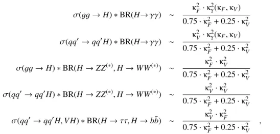
5.1.2 No assumption on the total width

The assumption on the total width gives a strong constraint on the fermion coupling scale factor

in the previous benchmark model, as the total width is dominated in the SM by the sum of the b, τ and gluon-decay widths. The fit is therefore repeated without the assumption on the total width.

In this case only ratios of coupling scale factors can be measured. Hence there are the following free parameters:

λFV = κF

/

(16)

κVV = κV

·

/

. (17)

λFV

is the ratio of the fermion and vector coupling scale factors, and

an overall scale that includes the total width and applies to all rates. For the most relevant Higgs boson production and decay modes the following proportionality is found:

σ(gg → H) ∗ BR(H→ γγ) ∼

·

·

(

, 1) σ (qq

→ qq

H) ∗ BR(H → γγ ) ∼

·

(

, 1)

σ ( gg → H) ∗ BR(H → ZZ

, H → WW

) ∼

·

(18) σ(qq

→ qq

H) ∗ BR(H → ZZ

, H → WW

) ∼

σ(qq

→ qq

H, V H) ∗ BR(H → ττ, H → b b) ¯ ∼

·

,

where the second order polynomial form of

(

,

), given in Equation (13), allows to factorize out the scale factor

into the common factor

and the ratio

as argument to the

function.

Figure 6 shows the results of this fit. The 68% confidence interval of

and

when profiling over the other parameter yield:

λFV

∈ [ − 0 . 94 , − 0 . 80] ∪ [0 . 67 , 0 . 93] (19)

∈ [0 . 96 , 1 . 12] ∪ [1 . 18 , 1 . 49] . (20) The two-dimensional compatibility of the SM hypothesis with the best fit point is 7%.

5.1.3 No assumption on the total width and on the

H → γγ

As the H→ γγ decay is loop induced, it can be a very sensitive probe of beyond the SM physics. There- fore the H→ γγ decay is treated in the following benchmark as additional degree of freedom. This gives the following benchmark model with the parameters of interest:

λFV = κF

/

(21)

λγV = κγ

/

(22)

κVV = κV

·

/

, (23)

where

is the ratio of the fermion and heavy vector coupling scale factors,

the ratio between the photon and vector coupling scale factors and

an overall scale that includes the total width and acts on all rates. For the most relevant Higgs boson production and decay modes the following proportionality is found:

σ ( gg → H) ∗ BR(H → γγ ) ∼

·

·

σ(qq

→ qq

H) ∗ BR(H→ γγ) ∼

·

σ ( gg → H) ∗ BR(H → ZZ

, H → WW

) ∼

·

(24) σ (qq

→ qq

H) ∗ BR(H → ZZ

, H → WW

) ∼

σ(qq

→ qq

H, V H) ∗ BR(H → ττ, H → b b) ¯ ∼

·

.

λFV

-1.5 -1 -0.5 0 0.5 1 1.5

) FVλ(Λ-2 ln

0 1 2 3 4 5 6 7 8 9 10

VV] κ

FV, λ [

Observed SM expected Ldt = 13-20.7 fb-1

∫

= 8 TeV, s

Ldt = 4.6-4.8 fb-1

∫

= 7 TeV, s

ATLAS Preliminary

(a)

κVV

0.6 0.8 1 1.2 1.4 1.6 1.8

FVλ

-1.5 -1 -0.5 0 0.5 1 1.5 2

2.5 SM

Best fit 68% CL 95% CL Ldt = 13-20.7 fb-1

∫ = 8 TeV, s

Ldt = 4.6-4.8 fb-1

∫ = 7 TeV, s

ATLAS Preliminary

(b)

κVV

0.4 0.6 0.8 1 1.2 1.4 1.6 1.8

)VVκ(Λ-2 ln

0 1 2 3 4 5 6 7 8 9 10

VV] κ

FV, λ [ Observed SM expected Ldt = 13-20.7 fb-1

∫ = 8 TeV, s

Ldt = 4.6-4.8 fb-1

∫ = 7 TeV, s

ATLAS Preliminary

(c)

Figure 6: Fits for a 2-parameter benchmark model described in Equations (16-18) probing di

erent coupling strength scale factors for fermions and vector bosons without assumptions on the total width:

(a) coupling scale factor ratio

(

is profiled); (b) correlation of the coupling scale factors

/

and

·

/

; (c) coupling scale factor ratio

(

is profiled). The dashed curves in (a) and (c) show the SM expectation. The thin dotted lines in (c) indicate the continuation of the likelihood curve when restricting the parameters to either the positive or negative sector of

.

λFV

0.4 0.6 0.8 1 1.2 1.4 1.6 1.8

) FVλ(Λ-2 ln

0 1 2 3 4 5 6 7 8 9 10

VV] κ

V, λγ FV, λ [

Observed SM expected Ldt = 13-20.7 fb-1

∫

= 8 TeV, s

Ldt = 4.6-4.8 fb-1

∫

= 7 TeV, s

ATLAS Preliminary

(a)

γV

λ

0.6 0.8 1 1.2 1.4 1.6 1.8

)Vγλ(Λ-2 ln

0 1 2 3 4 5 6 7 8 9 10

VV] κ

V, λγ FV, λ [ Observed SM expected Ldt = 13-20.7 fb-1

∫ = 8 TeV, s

Ldt = 4.6-4.8 fb-1

∫ = 7 TeV, s

ATLAS Preliminary

(b)

κVV

0.6 0.8 1 1.2 1.4 1.6

)VVκ(Λ-2 ln

0 1 2 3 4 5 6 7 8 9 10

VV] κ

V, λγ FV, λ [ Observed SM expected Ldt = 13-20.7 fb-1

∫ = 8 TeV, s

Ldt = 4.6-4.8 fb-1

∫ = 7 TeV, s

ATLAS Preliminary

(c)

Figure 7: Fits for a 3-parameter benchmark model described in Equations (21-24) probing di

erent

coupling strength scale factors for fermions, photons and heavy vector bosons without assumptions on

the total width: (a) coupling scale factor ratio

(

and

are profiled); (b) coupling scale factor

ratio

(

and

are profiled); (c) overall scale factor

(

and

are profiled). The dashed

curves show the SM expectation.