Measurements of Higgs boson properties in the diphoton decay channel using 80 fb−

A TLAS-CONF-2018-028 31/03/2019 A TLAS-CONF-2018-028 05 July 2018

ATLAS CONF Note

ATLAS-CONF-2018-028

5th July 2018

Measurements of Higgs boson properties in the diphoton decay channel using 80 fb ⁻¹ of p p collision data at √

s = 13 TeV with the ATLAS detector

The ATLAS Collaboration

This note reports measurements of Higgs boson properties in the two-photon final state us- ing 79.8 fb ^{− 1} of data recorded at √ s = 13 TeV by the ATLAS experiment at the Large Hadron Collider. The cross sections of Higgs boson production through gluon–gluon fusion, vector-boson fusion, and in association with a vector boson or a top-quark pair are measured.

Measurements of the Higgs boson production divided further into kinematic regions, called

simplified template cross sections, are also reported. Additionally, the cross section for the

production of the Higgs boson decaying to two isolated photons is measured in a fiducial

phase space designed to closely match the ATLAS detector acceptance, and is found to be

60.4 ± 6.1 (stat.) ± 6.0 (exp.) ± 0.3 (theo.) fb, in agreement with the Standard Model pre-

diction of 63.5 ± 3.3 fb. Finally, the fiducial cross section is measured differentially in bins

of several kinematic observables with sensitivity to properties of the Higgs boson. Among

these, the number of b-jets produced in association with the Higgs boson is measured to

probe Higgs production in association with heavy flavor hadrons. No significant deviations

between the observed data and the Standard Model prediction are observed.

1 Introduction

In 2012, the ATLAS [1] and CMS [2] collaborations announced the discovery of the Higgs boson [3, 4]. Subsequent measurements have sought to characterize the properties of the Higgs boson and its production mechanisms. This year (2018), the observation of Higgs boson production in association with a top quark pair was reported by both CMS and ATLAS [5, 6]. Higgs boson properties have been previously measured in the diphoton decay channel at √ s = 13 TeV [7, 8]; in 2017, ATLAS recorded an additional 43.6 fb ⁻¹ of good quality data, allowing for roughly a 50% improvement in statistical precision compared to the previous measurement [7].

This note reports measurements of the properties of the Higgs boson decaying to two photons, using 79.8 fb ⁻¹ of pp collision data collected by the ATLAS detector between 2015 and 2017. The cross sections of the Higgs production modes are measured inclusively and in kinematic phase space regions known as simplified template cross sections (STXS) [9, 10]. The cross section is also measured inclus- ively in a fiducial phase space designated to match the selection at reconstruction level, and corrected for detector effects to the particle level. Within this phase space, the Higgs boson signal is measured differentially in bins of kinematic observables that shed light on its properties. In addition, the number of b-jets is measured in a fiducial region containing one or more central jets and no electrons or muons, in order to probe Higgs boson production in association with heavy-flavor hadrons (excluding t tH ¯ ). All measurements are compared to Standard Model (SM) theoretical predictions.

The measurements presented in this note follow a methodology that is largely unchanged since Ref. [7];

differences are highlighted in the text. A notable exception is the re-optimization of the measurement of the top-associated production mode, which is documented as part of the ATLAS observation of t¯ tH production [6] and summarized in this note. Despite sharing the same methodology and data set, the measurement of the t tH ¯ production mode in this note differs from Ref. [6] due to a different treatment of the other production modes, which were fixed to the SM prediction in Ref. [6] and are fit to data here, and due to different effects of the systematic uncertainties derived from the fit of additional categories. The fiducial measurement of the number of b-jets is also new in this note.

The note is organized as follows. The remainder of this section introduces the general analysis strategy.

Section 2 briefly describes the ATLAS detector, and Section 3 defines the data set used for these results.

Section 4 describes the simulated samples used for the measurements. Section 5 outlines the procedure

to reconstruct objects and events in the data set. The modeling of signal and background processes

and the statistical methods used for interpreting the results are described in Section 6. The systematic

uncertainties are described in Section 7. The results of the production mode and simplified template cross

section measurements are reported in Section 8, and findings of the inclusive fiducial and differential

cross section measurements are reported in Section 9. Section 10 summarizes the main conclusions of

the results.

1.1 Higgs boson production mode cross sections and simplified template cross sections In this note, for Higgs boson absolute rapidity1 | y H | < 2.5, cross sections are measured for several pro- duction modes of the Higgs boson: gluon–gluon fusion (ggF), vector-boson fusion (VBF), Higgs boson production in association with a vector boson (V H : sum of W H, q q ¯ ⁰ → Z H, and gg → Z H processes), and Higgs boson production in association with a top–antitop quark pair (t tH) or a single top quark (tH: ¯ sum of t-channel process tHq and W-associated process tHW). Higgs boson production in association with a bottom–antibottom quark pair (b bH) is merged with ggF, because it is expected to have small ¯ contributions, and similar kinematics and acceptance to ggF. In addition, the signal strength, defined as the ratio of the observed to expected event yield, is measured for inclusive Higgs production.

Furthermore, the simplified template cross sections introduced in Refs. [9, 10] are investigated. For

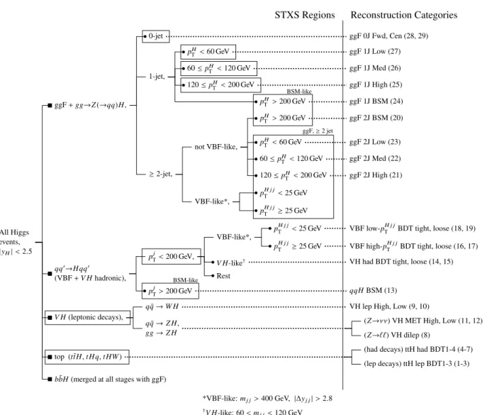
| y _H | < 2.5, the different Higgs boson production modes are separated into fiducial regions of phase space using the kinematics and topology of the final state, defined by the Higgs boson, the vector bosons or top quarks, and the hadronic jets in the event. The SM predictions of the Higgs boson production modes are used as “templates” for those fiducial regions. The template cross section measurements are designed to proceed in stages: “stage 0” is defined using the five main production modes (ggF, VBF, V H (leptonic decays), top-associated production, and b bH); “stage 1” divides these regions further based on event kin- ¯ ematic properties, to be measured when the experimental sensitivity allows. In the simplified template cross section framework, the W H and q q ¯ ⁰ → Z H processes with the vector boson decaying hadronically are grouped with the VBF production mode, and the gg → Z H process with the Z boson decaying had- ronically is grouped with the ggF production mode. This organization is different from the one used in the production mode cross section measurements. Additionally, because the current data set is not large enough to probe all 31 stage-1 cross sections, regions with poor sensitivity or with large anti-correlations are merged together, such that 9 cross section regions are measured.

Figure 1 and Table 1 summarize the stage-0 and stage-1 cross sections relevant to this measurement and indicate the 9 measured cross sections. The diphoton events are divided into 29 categories based on the reconstructed event properties, to target the different production modes and the different simplified template cross section regions. These event reconstruction categories are also shown in Figure 1, and discussed in Section 8.

1.2 Fiducial integrated and di ff erential cross sections

The pp → H → γγ cross section is measured in a fiducial region matching the selection imposed at recon- struction level and reported both as an integrated cross section and in di ff erential measurements. The diphoton fiducial region used for the inclusive measurement is defined at the particle level by requiring two photons, not originating from hadrons, that are each required to have an absolute pseudorapidity

| η | < 2 . 37 and outside the region 1 . 37 < | η | < 1 . 52. The two photons with the highest transverse mo- menta define the diphoton system. The leading (subleading) photon must have a transverse momentum greater than 35% (25%) of the mass of the diphoton system, m γγ . Both photons must be isolated from other activity using a particle-level isolation requirement. The kinematic and isolation requirements of

1

The ATLAS experiment uses a right-handed coordinate system with its origin at the nominal interaction point (IP) in the

center of the detector and the z-axis along the beam pipe. The x-axis points from the IP to the center of the LHC ring, and the

y-axis points upward. Cylindrical coordinates (r, φ) are used in the transverse plane, φ being the azimuthal angle around the

z-axis. The pseudorapidity is defined in terms of the polar angle θ as η = − ln tan(θ/2). When dealing with massive particles,

the rapidity y = 1/2 ln[(E + p

)/( E − p

)] is used, where E is the energy and p

is the z-component of the momentum.

All Higgs events,

|y_H|<2.5

ggF+gg!Z(!qq)H,

0-jet ggF 0J Fwd, Cen (28, 29)

1-jet,

p_T^H<60 GeV ggF 1J Low (27)

60p_T^H<120 GeV ggF 1J Med (26)

120p_T^H<200 GeV ggF 1J High (25) p_T^H>200 GeV ggF 1J BSM (24)

2-jet,

not VBF-like,

p_T^H>200 GeV ggF 2J BSM (20)

p_T^H<60 GeV ggF 2J Low (23) 60p_T^H<120 GeV ggF 2J Med (22) 120p_T^H<200 GeV ggF 2J High (21)

VBF-like*, p_T^{H j j}<25 GeV p_T^{H j j} 25 GeV

qq⁰!Hqq⁰

(VBF+V Hhadronic),

p_T^j<200 GeV,

VBF-like*, p^{H j j}_T <25 GeV VBF low-p_T^{H j j}BDT tight, loose (18, 19) p^{H j j}_T 25 GeV VBF high-p^{H j j}_T BDT tight, loose (16, 17) V H-like^† VH had BDT tight, loose (14, 15) Rest

p_T^j>200 GeV qqHBSM (13)

V H(leptonic decays),

qq¯!W H VH lep High, Low (9, 10)

qq¯!Z H, gg!Z H

(Z!⌫⌫) VH MET High, Low (11, 12)

(Z!``) VH dilep (8)

top (t¯tH,tHq,tHW) (had decays) ttH had BDT1-4 (4-7)

(lep decays) ttH lep BDT1-3 (1-3) bbH¯ (merged at all stages with ggF)

BSM-like

BSM-like

ggF, 2 jet

Reconstruction Categories STXS Regions

*VBF-like:mj j>400 GeV, | yj j|>2.8

†V H-like: 60<mj j<120 GeV

Figure 1: The particle-level kinematic regions relevant to this measurement, as defined by the simplified template

cross section (STXS) framework. Stage-0 simplified template cross section regions are indicated with an adjacent

square; stage-1 regions are denoted with a circle. Some stage-1 regions are omitted from the figure in cases where

the data set lacks the sensitivity to resolve them. The event reconstruction categories targeting specific particle-level

kinematic regions, defined in Table 3, are listed to the right of each region. Events in data are assigned preferentially

to categories starting from “ttH lep BDT1” and using the order indicated by the numbers in parentheses (note that

the ggF categories are mutually exclusive of one another). Though some of the non-t tH ¯ category names have

changed, the definition of those categories is the same as in Ref. [7]. The particle-level regions are merged to form

9 intermediate regions, indicated with rectangular boxes, whose cross sections are measured in this note. Note that

one disjoint region (“BSM-like”) is denoted by two labeled boxes.

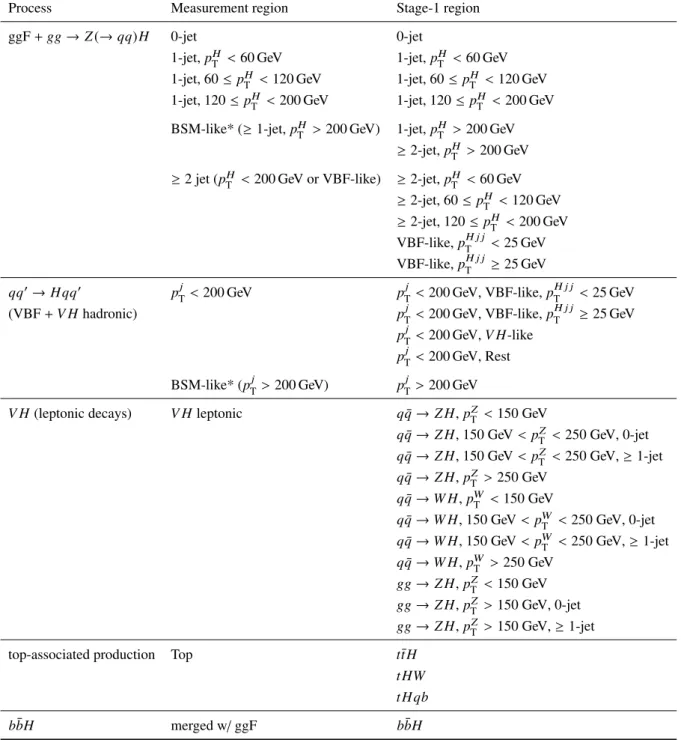
Process Measurement region Stage-1 region

ggF + gg → Z( → qq)H 0-jet 0-jet

1-jet, p

< 60 GeV 1-jet, p

< 60 GeV 1-jet, 60 ≤ p

< 120 GeV 1-jet, 60 ≤ p

< 120 GeV 1-jet, 120 ≤ p

< 200 GeV 1-jet, 120 ≤ p

< 200 GeV BSM-like* ( ≥ 1-jet, p

> 200 GeV) 1-jet, p

> 200 GeV

≥ 2-jet, p

> 200 GeV

≥ 2 jet (p

< 200 GeV or VBF-like) ≥ 2-jet, p

< 60 GeV

≥ 2-jet, 60 ≤ p

< 120 GeV

≥ 2-jet, 120 ≤ p

< 200 GeV VBF-like, p

< 25 GeV VBF-like, p

≥ 25 GeV

qq

→ Hqq

p

< 200 GeV p

< 200 GeV, VBF-like, p

< 25 GeV (VBF + V H hadronic) p

< 200 GeV, VBF-like, p

≥ 25 GeV

p

< 200 GeV, V H-like p

< 200 GeV, Rest BSM-like* (p

> 200 GeV) p

> 200 GeV

V H (leptonic decays) V H leptonic q q ¯ → Z H, p

< 150 GeV

q q ¯ → Z H, 150 GeV < p

< 250 GeV, 0-jet q q ¯ → Z H, 150 GeV < p

< 250 GeV, ≥ 1-jet q q ¯ → Z H, p

> 250 GeV

q q ¯ → W H , p

< 150 GeV

q q ¯ → W H , 150 GeV < p

< 250 GeV, 0-jet q q ¯ → W H , 150 GeV < p

< 250 GeV, ≥ 1-jet q q ¯ → W H , p

> 250 GeV

gg → Z H, p

< 150 GeV gg → Z H, p

> 150 GeV, 0-jet gg → Z H, p

> 150 GeV, ≥ 1-jet

top-associated production Top t¯ tH

tHW tHqb

b bH ¯ merged w/ ggF b bH ¯

Table 1: The kinematic regions of the stage-1 simplified template cross sections. The left column indicates the five main production modes, the middle column describes the 9 measurements probed in this result, and the right column lists the stage-1 template cross sections and their relation to the measurements. Note that the cross section of the sum of the two measurement regions labeled “BSM-like” (marked with an asterisk) is reported. All regions require | y

| < 2.5. Jets are defined using the anti-k

algorithm with radius parameter R = 0.4 and are required to have p

> 30 GeV. The leading jet and Higgs boson transverse momenta are denoted by p

and p

, respectively.

The transverse momentum of the Higgs boson and the leading and subleading jet is denoted as p

. Events are

considered “VBF-like” if they contain at least two jets with an invariant mass of m

> 400 GeV and a rapidity

seperation between the two jets of | ∆y

| > 2.8. Events are considered “V H -like” if they contain at least two jets

with an invariant mass of 60 GeV < m

< 120 GeV. All qq

→ Hqq

VBF and V H events (with the vector boson

V decaying hadronically) which are neither VBF nor V H-like are part of the “Rest” selection.

the fiducial selection are defined to mimic the event selection imposed on data in order to minimize any uncertainty associated with extrapolating outside the detector fiducial volume. Electrons, muons and jets are also defined at the particle level as described in detail in Section 9.

Using the diphoton fiducial region defined above, the following distributions are measured di ff erentially at the particle level:

• p ^γγ _T , the transverse momentum of the diphoton system,

• | y γγ | , the rapidity of the diphoton system,

• p _T ^j

, the transverse momentum of the leading jet,

• N b-jets , the number of central jets2 containing a b-hadron, in a fiducial region described below.

The distribution of N b-jets is measured in a fiducial region designed to probe Higgs boson production in association with heavy-flavor particles, which is poorly constrained theoretically, and which is an important background in measurements and searches for t tH ¯ and H H production. In order to specifically target Higgs boson production in association with heavy-flavor particles and reduce the fraction of t¯ tH events, the fiducial region for this measurement is constructed using a veto on electrons and muons.

In addition, at least one central jet with transverse momentum p T > 30 GeV is required to match the acceptance of the inner detector.

2 ATLAS detector

The ATLAS detector [1] covers almost the entire solid angle around the proton–proton interaction point.

It consists of an inner tracking detector, electromagnetic and hadronic calorimeters, and a muon spectro- meter.

The inner detector (ID), immersed in a 2 T axial magnetic field provided by a superconducting solen- oid, provides precision tracking for charged particles ( | η | < 2.5). The ID consists of a silicon pixel detector (including the insertable B-layer [11]), a silicon microstrip detector (SCT), and a transition radi- ation tracker (TRT). The ID is surrounded by the electromagnetic (EM) and hadronic calorimeters. The EM calorimeter is a lead/liquid-argon (LAr) sampling calorimeter, measuring electromagnetic showers in the barrel ( | η | < 1.475) and endcap (1.375 < | η | < 3.2) regions. The hadronic calorimeter recon- structs hadronic showers using steel and scintillator tiles ( | η | < 1 . 7), copper/LAr (1 . 5 < | η | < 3 . 2), or copper–tungsten/LAr (3.1 < | η | < 4.9). A muon spectrometer (MS) surrounds the calorimeter system.

It comprises separate trigger chambers ( | η | < 2.4) and precision tracking chambers ( | η | < 2.7), in a magnetic field provided by three superconducting air-core toroids.

ATLAS data-taking uses a two-level trigger system [12]: a hardware-based first-level (L1) trigger com- ponent, reducing the event rate to at most 100 kHz, and a software-based high-level trigger component, reducing the event rate to approximately 1 kHz.

2

Central jets are defined as having | y | < 2.5, matching the acceptance of the inner detector.

3 Data set

This study uses a data set of √ s = 13 TeV proton-proton collisions recorded by the ATLAS detector from 2015 to 2017. After data quality requirements are applied to ensure good working condition of all detector components, the data set amounts to an integrated luminosity of 79.8 ± 1.6 fb ⁻¹ . The mean number of interactions per bunch crossing was on average < µ> = 24 combining data collected in 2015 and 2016, and in 2017 it increased to < µ> = 38. Events are selected by a diphoton trigger with transverse energy thresholds of 35 GeV and 25 GeV for the leading and subleading photon candidates, respectively.

The photon identification requirements of this trigger were tightened in 2017 to cope with a higher in- stantaneous luminosity. On average, the trigger has an efficiency greater than 98% for events that pass the diphoton event selection described in Section 5.

4 Event simulation

Signal events from ggF, VBF, V H , t tH ¯ and b bH ¯ production modes are generated using Powheg [13–20], with the PDF4LHC15 PDF set [21], and interfaced to Pythia8 [22, 23] for parton showering, hadroniza- tion and underlying event using the AZNLO set of parameters that are tuned to data [24]. tH processes are modeled using Madgraph5_aMC@NLO [25] with the CT10 PDF set [26]. tHq events are passed to Pythia8 with the A14 parameter set [27], while tHW events are interfaced to Herwig++ [28–30] with the Herwig++ UEEE5 parameter set. The generated signal events are passed through a Geant4 [31] simula- tion of the ATLAS detector response. The cross sections of Higgs production processes are reported for a center-of-mass energy of √ s = 13 TeV and a SM Higgs with mass 125.09 GeV. These cross sections [9, 32–49], along with the Higgs branching ratio to diphotons (0.227%) [9, 50–54], are used to normalize the simulated signal events.

Background events from continuum γγ production and V γγ production are generated using Sherpa 2.2.4 [55], and merged with the Sherpa parton shower [56] according to the ME+PS@NLO prescrip- tion [57]. The CT10 PDF set and dedicated parton shower tuning developed by the Sherpa authors are used. t tγγ ¯ production is modeled using Madgraph5_aMC@NLO interfaced to Pythia8, with the PDF4LHC15 PDF set and the A14 parameter set. The background samples are passed through a fast parametric simulation of the ATLAS detector response [58].

Additional proton-proton interactions (pile-up) are produced using Pythia8 with the A2 parameter set [59]

and the MSTW2008lo PDF set [60]. They are included in the simulation for all generated events such that the distribution of the mean number of interactions per bunch crossing reproduces that observed in the data.

A summary of the simulated signal and background samples is shown in Table 2.

5 Event reconstruction and selection

Collision events are reconstructed in the ATLAS detector using a series of object reconstruction al- gorithms, summarized below. Events in this analysis are selected using the following procedure: first, reconstructed photon candidates are required to satisfy a set of preselection-level identification criteria.

The two highest-p T preselected photons are used to define the diphoton system, and an algorithm is used

Process Generator Showering PDF set √ s σ = [pb] 13 TeV Order of σ calculation ggF P owheg NNLOPS P ythia 8 PDF4LHC15 48.52 N

LO(QCD)+NLO(EW) VBF Powheg-Box Pythia 8 PDF4LHC15 3.78 approximate-NNLO(QCD)+NLO(EW)

W H Powheg-Box Pythia 8 PDF4LHC15 1.37 NNLO(QCD)+NLO(EW)

q q ¯

→ Z H Powheg-Box Pythia 8 PDF4LHC15 0.76 NNLO(QCD)+NLO(EW)

gg →Z H Powheg-Box Pythia 8 PDF4LHC15 0.12 NNLO(QCD)+NLO(EW)

t tH ¯ Powheg-Box Pythia 8 PDF4LHC15 0.51 NNLO(QCD)+NLO(EW)

b bH ¯ Powheg-Box Pythia 8 PDF4LHC15 0.49 NNLO(QCD)+NLO(EW)

tHq MG5_ a MC@NLO P ythia 8 CT10 0.07 4FS(LO)

tHW MG5_aMC@NLO Herwig++ CT10 0.02 5FS(NLO)

γγ Sherpa Sherpa CT10

V γγ Sherpa Sherpa CT10

t¯ tγγ MG5_aMC@NLO Pythia 8 PDF4LHC15

Table 2: Event generators and PDF sets used to model signal and background processes. The cross sections of Higgs production processes [9, 32–49] are reported for a center of mass energy of √ s = 13 TeV and a SM Higgs with mass 125.09 GeV. The order of the calculated cross section is reported in each case. The cross sections for the background processes are omitted, because the background normalisation is determined in fits to the data.

to select the diphoton primary vertex among the reconstructed vertices. Finally, the photons are required to satisfy isolation and additional identification selection criteria. Additional objects (jets, muons, elec- trons, and missing energy) are also reconstructed and identified for the purpose of further categorizing the events and measuring Higgs boson properties.

5.1 Photon reconstruction and identification

Photons are reconstructed from calorimeter clusters formed using a dynamical, topological cell clustering- based algorithm [61, 62]. The photon candidate is classified as converted if two tracks forming a con- version vertex, or one track with the signature of an electron track but without hits in the innermost pixel layer, are matched to it; otherwise it is labeled as unconverted. The photon candidate energy is calibrated using a procedure developed in Run 1 [63] and re-optimized for 13 TeV data [64].

Reconstructed photons must satisfy | η | < 2 . 37 in order to fall inside the region of the EM calorimeter with a finely segmented layer, and outside the range 1.37 < | η | < 1.52 corresponding to the transition region of the barrel and endcap EM calorimeters. Photon candidates are separated from jet backgrounds using an identification criteria based on calorimeter shower shape variables [61, 65]. A loose working point is used for preselection, and the final selection of photon candidates is made using a tight selection.

For photons above 25 GeV, the efficiency of the tight identification ranges from about 84% to 94% (85%

to 98%) for unconverted photons (converted photons).

The final selection of photons includes calorimeter- and track-based isolation requirements to further suppress jets misidentified as photons. The calorimeter isolation variable is defined as the energy in the EM calorimeter in a radius ∆ R = 0 . 2 around the photon candidate, excluding the energy associated to the photon candidate and correcting for pile-up and underlying event contributions [65, 66]. The calorimeter- based isolation must be less than 6.5% of the photon transverse energy for each photon candidate. The track-based isolation variable is defined as the scalar sum of the transverse momenta of tracks with a radius

∆R < 0.2 around the photon candidate. The tracks considered in the isolation variable are restricted to

those with p T > 1 GeV that are associated to the selected diphoton primary vertex and not associated

0 10 20 30 40 50 60 µ 0

20 40 60 80 100

Fraction [%]

Preliminary

ATLAS s = 13 TeV, 79.8 fb

γ

γ Stat. Unc.

γ j Tot. Unc.

jj

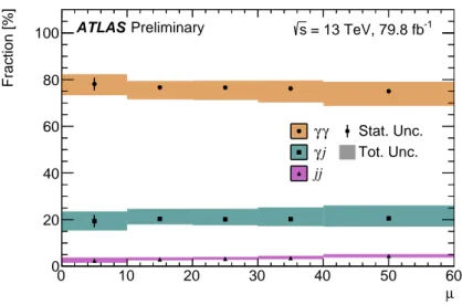
Figure 2: The purity of γγ events in the diphoton fiducial region, measured in bins of µ (the mean number of interactions per bunch crossing). The fraction of γγ, γ j and j j events in each µ region is measured using the procedure described in Section 6.2.

with a photon conversion vertex. Both photons must have a track isolation less than 5% of the photon transverse energy.

5.2 Event selection and selection of the diphoton primary vertex

Events are selected by first requiring at least two photons satisfying the loose identification preselection criteria. The two highest-p T preselected photons are designated as the candidates for the diphoton system, and all other photon candidates are discarded. The measured trajectory of these two photons, along with the reconstructed vertex information in the event, are used as inputs to a neural-network algorithm trained on simulation to determine the correct primary vertex [67]. This algorithm has been shown to select the correct primary vertex (within 0.3 mm of the true vertex) in simulated gluon-fusion signal events 76%

of the time. Its performance was validated using Z → ee events in data and simulation, ignoring the track information of the electrons and treating them as photon candidates [68]. The two preselected photon candidates are required to satisfy the tight identification criteria and the isolation selection described above. Finally, the leading and subleading photon candidates are required to satisfy p T /m γγ > 0.35 and 0.25, respectively.

The trigger, object and event selection described up until now are used to define the events that are selected for further analysis for Higgs boson properties. In total, 733455 events are selected in this data set with a diphoton invariant mass between 105 and 160 GeV. The predicted signal efficiency, assuming a SM Higgs boson and including the fiducial acceptance of the kinematic selection, is 34%.

With respect to the previous analysis, which used data collected in 2015 and 2016, the additional data

collected in 2017 features higher pile-up conditions. Despite this increase in pile-up, the purity of γγ

events with respect to events with one or two jets reconstructed as photons is fairly stable. Figure 2

illustrates the purity of γγ events in bins of µ as measured by the background composition procedure

described in Section 6.2.

5.3 Reconstruction and selection of hadronic jets, b-jets, leptons and missing transverse momentum

Jets are reconstructed from topological clusters in the calorimeters using the anti-k t algorithm with radius parameter 0.4 [69]. Jets are required to have | η | < 4.4, as well as p T > 25 or 30 GeV depending on the measurement performed. Jets originating from pile-up collisions in the range | η | < 2 . 4 and p T < 60 GeV are suppressed using a jet vertex tagger multivariate discriminant [70, 71]. Jets with | η | < 2 . 5 containing b-hadrons are identified using the MV2c10 b-tagging algorithm with a working point selected to achieve a 70% or 77% b-tagging efficiency [72, 73] depending on the measurement.

Electrons are constructed by matching tracks in the ID to topological calorimeter clusters formed using the same dynamical, topological cell clustering-based algorithm as in the photon reconstruction [62, 74].

Electron candidates are required to have p T > 10 GeV, | η | < 2 . 47 and must satisfy a selection based on a likelihood discriminant made from calorimeter shower shapes and track parameters [75]. Isolation criteria are applied to electrons using calorimeter- and track-based information using a selection designed to obtain a flat efficiency of 99% in all ranges of η and p T . The reconstructed track associated to the electron candidate must be consistent with the diphoton vertex by requiring its longitudinal impact parameter z 0

relative to the vertex to satisfy | z 0 sin θ | < 0.5 mm. In addition, the electron transverse impact parameter with respect to the beam axis divided by its uncertainty, | d 0 | /σ _d

, must be less than 5.

Muons are reconstructed by matching tracks from the MS and ID subsystems. Muons without an ID track but whose MS track is compatible with the interaction point are also considered. Muon candidates are required to have p T > 10 GeV, | η | < 2 . 7, and must satisfy the medium identification requirements [76]. Muons are required to satisfy calorimeter- and track-based isolation requirements that are 95-97%

efficient for muons with p T ∈ [10, 60] GeV and 99% efficient for p T > 60 GeV. Muon tracks must satisfy

| z 0 sin θ | < 0 . 5 mm and | d 0 | /σ _d

< 3.

An overlap removal procedure is performed in order to avoid double-counting objects, using the quantity

∆R = p

∆φ ² + ∆y ² . First, electrons overlapping with the two selected photons (∆R < 0.4) are removed.

Jets overlapping with the selected photons ( ∆ R < 0 . 4) and electrons ( ∆ R < 0 . 2) are removed. Electrons overlapping with the remaining jets (∆R < 0.4) are removed to match the requirements imposed when measuring isolated electron efficiencies. Finally, muons overlapping with photons or jets (∆R < 0.4) are removed.

The missing transverse momentum is defined as the negative vector sum of the transverse momenta of the selected photon, electron, muon and jet objects, as well as of the transverse momenta of remaining low-p T particles estimated using tracks associated to the primary vertex but not assigned to any of the above selected objects [77].

6 Signal and background modeling

The Higgs boson signal yield is extracted using a maximum likelihood fit to the diphoton invariant mass spectrum in each event reconstruction category and differential cross-section bin, and in the diphoton fiducial region (which are defined in Sections 8 and 9). The fit is performed on data in the range 105 <

m γγ < 160 GeV using parameterized models for signal and background. The signal and background

modeling follows the methodology described in Ref. [7] and is summarized below.

115 120 125 130 135 140 [GeV]

γ

m

0 0.02 0.04 0.06 0.08 0.1 0.12 0.14 0.16

/ 0.5 GeV

m 1/N dN/d

Simulation Preliminary ATLAS

= 13 TeV s = 125 GeV , mH

γ γ

→

= 1.7 GeV σ68

ggF 0J CEN, MC Signal Model

= 2.1 GeV σ68

ggF 0J FWD, MC Signal Model

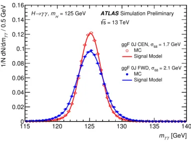
Figure 3: Simulated signal events and the fitted signal parameterization for two event categories. The ggF 0J Cen category has among the best mass resolutions, and the ggF 0J Fwd region has the worst mass resolution of the measured categories.

6.1 Signal model

The Higgs boson signal is modeled as a double-sided Crystal Ball function, with the bulk of the distribu- tion modeled by a Gaussian distribution and upper and lower tails described using power-law functions [78, 79]. The parameters of the signal model are obtained using a fit to the simulated Higgs samples in each differential bin and event reconstruction category, and in the diphoton fiducial region. Figure 3 depicts the signal model parameterizations for two event categories having among the best (ggF 0J Cen), and the worst (ggF 0J Fwd) mass resolutions. The effective signal mass resolutions of these categories, defined as half the smallest m γγ window containing 68% of signal events, are 1.7 and 2.1 GeV, respect- ively. Table 11 in the appendix reports the effective signal mass resolutions in all 29 reconstruction categories.

6.2 Background model and composition

The background is modeled in each event region or category using either a power law function, a fourth- order Bernstein polynomial, or an exponential of a first-, second-, or third-order polynomial. Background functions are chosen in each region to ensure a small potential bias on the measured signal yield while keeping the number of degrees of freedom small to reduce the statistical uncertainty. The procedure to measure the possible bias, and thus to make the choice of function, is performed using fits of the signal plus background model to a sample representing the background-only invariant mass spectrum.

The background samples used to perform the bias tests and determine the background functional form are

taken from data control regions or simulated samples, depending on the region. For fiducial differential

bins, ggF categories, VBF categories, and V H hadronic categories, which are dominated by γγ, γ j and j j

backgrounds, the simulated Sherpa γγ events are used as a background model. This sample is corrected

to reflect the shape differences of γ j and j j and taking into account the relative event fractions of γγ, γ j and j j in each region.

To measure the relative γγ, γ j and j j event fractions in each region, a double two-dimensional sideband method [66, 80] is applied using data control regions in which the nominal identification and isolation requirements are relaxed. To determine the shape difference between Sherpa γγ and γ j, the simulated γγ shape is compared to a control region in which the identification criteria of exactly one of the two photons is inverted; contamination from γγ in this region is subtracted, and a linear reweighting is derived to match the γγ and control region shapes. The procedure is repeated in a control region in which the identification criteria of both photons is inverted to determine a shape reweighting for j j events. These derived shapes are combined with the measured relative event fractions to obtain the total background shape. In the inclusive sample of selected events with diphoton invariant mass between 105 and 160 GeV, the γγ fraction is measured to be 75.6 ^+3.1 _{− 4.8} %; the error is dominated by the systematic uncertainty. Figure 2 in Section 5 reports the purity of γγ events in bins of the mean number of interactions per bunch crossing.

Background templates for categories targeting V H signal decaying to charged or neutral leptons are obtained using simulated V γγ and γγ background samples, combined according to the predicted cross sections. Categories targeting leptonic tH and t tH ¯ decay modes use simulated t t ¯ γγ samples to model the background.

For categories targeting tH and t¯ tH production with hadronically decaying top quarks, data control re- gions are obtained using events in which at least one of the two photons fails either isolation or identi- fication selection criteria, and the requirement on the number of b-tagged jets is removed, but satisfying all other selection criteria. These templates are validated by verifying that their shape describes the data in the diphoton invariant mass ranges 105 < m γγ < 120 GeV and 130 < m γγ < 160 GeV of the signal region.

In each category or region, signal plus background fits are performed on the background-only templates described above using candidate background functions and the parameterized signal model. The absolute value of the amount of signal fitted in a signal plus background fit is a measure of the potential bias caused by the choice of background function. The maximum of this quantity from a series of fits scanning the parameterized signal mass in the range 121-129 GeV, called the spurious signal, is the metric used to describe the systematic uncertainty due to the choice of background function.

If the spurious signal of a background function is less than 10% of the expected SM Higgs yield, or less than 20% of the expected error on the measured signal yield, or if the spurious signal is consistent with satisfying one of these criteria within 2σ of the statistical uncertainty on the estimated spurious signal, then the function is considered as a background model. The statistical uncertainty on the estimated spuri- ous signal is caused by the finite size of the background sample used to perform the test. Furthermore, a background-only fit of the function to the background sample must satisfy a loose χ ² requirement, p( χ ² ) > 0 . 01.3 Among the functions satisfying these criteria in a given region or category, the function with the smallest number of parameters is chosen. In case two candidate functions have the same num- ber of parameters, the function with the smallest spurious signal is chosen. The selected functions have between 1 and 4 degrees of freedom (excluding the parameter used to normalize to data), depending on the category, bin, or region.

3

In a few differential bins and categories, p( χ

) requirement fails for all candidate functions due to random fluctuations in the

background sample. The requirement is dropped in these individual cases.

6.3 Statistical Model

The statistical procedure used to interpret the data is described in Ref. [81] and follows the methods from Ref. [7]. For each measurement, signal yields are determined using the maximum profile likelihood ratio for an extended likelihood function. The likelihood functions used in each measurement are described below.

For the inclusive fiducial measurement, the likelihood function is built from the diphoton invariant mass distribution of data events in the range m γγ ∈ [105 , 160] GeV and satisfying the diphoton fiducial region requirements. The signal and background parameterizations determined for the inclusive measurement are used to model the data in the likelihood.

Similarly, in each bin and category, and in the diphoton fiducial region, an extended likelihood function is constructed from the m γγ distribution of data events in the range m γγ ∈ [105, 160] GeV, modeled using the signal and background parameterizations derived for each region. The likelihood used in the production mode and simplified template cross section measurements is the product of extended likelihood functions from each reconstruction category. For each differential cross section measurement, the likelihood is taken as the product of extended likelihood functions from each bin in the distribution.

Systematic uncertainties are incorporated into the likelihood function of each bin, category and region using a set of Gaussian or log-normal constraints on nuisance parameters. The full list and treatment of systematic uncertainties is discussed in Section 7.

7 Systematic uncertainties

Systematic uncertainties considered in this analysis can be grouped into three categories: (i) uncertainties in the signal and background modeling of the m γγ spectrum, (ii) experimental uncertainties affecting the expected signal yields in each reconstruction category and di ff erential bin, and in the diphoton fiducial region, and (iii) theoretical uncertainties in the signal yield modeling. These systematic uncertainties are discussed in the following sections.

The measurements based on event reconstruction categories incorporate the yield uncertainties and the m γγ spectrum uncertainties directly into the likelihood function (described in Section 6.3), which is used to extract the signal strength or cross section. For the measurements of fiducial and differential cross sections, the likelihood function is constructed using only the uncertainties in the modeling of the m γγ

spectrum to extract the signal events, and yield uncertainties are incorporated at a later stage as part of a correction factor (introduced in Section 9.2) or part of the luminosity. Theoretical uncertainties are also evaluated differently as discussed in Sections 7.3 and 7.4.

7.1 Systematic uncertainties in the signal and background modeling of the m _γγ spectrum The photon energy scale uncertainties shift the position of the signal peak by between ± 0.2% and ± 0.4%, while the photon energy resolution uncertainties change the width of the signal peak by between ± 6%

and ± 15%, following Refs. [64, 82]. These uncertainties are implemented as independent sources of

systematic uncertainty. Another uncertainty affecting the signal peak position is the uncertainty due to

the knowledge of the Higgs boson mass of 0.24 GeV [83].

The uncertainty due to the background function choice is taken to be the spurious signal yield discussed in Section 6.2, and assumed to be uncorrelated between categories.

7.2 Experimental systematic uncertainties a ff ecting the expected signal yields

The uncertainty in the combined 2015-2017 integrated luminosity is 2.0%. It is derived, following a methodology similar to that detailed in Ref. [84], from a preliminary calibration of the luminosity scale using x-y beam-separation scans.

Other sources of experimental uncertainties affecting the expected signal yields include: the efficiency of the diphoton trigger [12], the photon identification efficiencies [61], the photon isolation efficiencies, the photon energy scale and resolution [64, 82], the modeling of pile-up in the simulation, the jet energy scale and resolution [69, 85, 86], the efficiency of the jet vertex tagger, the efficiency of the b-tagging algorithm [87], the electron [75] and muon [76] reconstruction, identification and isolation efficiencies, the electron [64] and muon [76] energy and momentum scale and resolution, as well as the contribu- tion to E _T ^miss from charged-particle tracks that are not associated with high-p T electrons, muons, jets, or photons [77]. Among these, the uncertainties with the largest variations in signal yields are the jet energy scale and resolution uncertainties (up to 24%) and photon isolation efficiency uncertainties (4-5%).

7.3 Theoretical modeling uncertainties for production mode and simplified template results

For the production mode and simplified template cross section measurements, the theoretical modeling uncertainties affecting the acceptance and efficiency of Higgs boson production processes include those due to:

• missing higher-order terms in the perturbative QCD calculations, estimated by varying the renor- malization and factorization scales. For the gluon–gluon fusion process, nine additional uncertainty sources are included for the missing higher-order QCD corrections: four sources [9, 88–90] account for modeling uncertainties in the jet multiplicities; three sources parameterize modeling uncertain- ties in the Higgs boson p T ; two sources [91, 92] account for the uncertainty in the acceptance of gluon–gluon fusion events in the VBF categories. The variations due to these uncertainties range from less than 1% to 27%.

• the choice of parton distribution functions and the value of α _S , estimated using the PDF4LHC15 recommendations [21]. Their effects are usually small.

• the modeling of the parton shower, underlying event, and hadronization, assessed by comparing the acceptance of simulated signal samples showered with Pythia to that of samples showered with Herwig. For the ggF process, the effects of the eigenvector tunes from the AZNLO set are merged to provide one additional uncertainty. The variations due to these uncertainties range from less than 1% to 18%.

Finally, in the categories targeting the t tH ¯ processes, the predicted ggF, VBF and V H yields are each

assigned a conservative 100% uncertainty (correlated between categories), which is due to the theoretical

uncertainty in the radiation of additional heavy-flavor jets in these Higgs boson production modes. This is

supported by measurements using H → Z Z ^∗ → 4 ` [93], t tb ¯ b ¯ [94], and V b [95, 96] events, and is consistent

with the N b-jets measurement reported in Section 9.4. The impact of this uncertainty on the results is small, due to the high t tH ¯ signal purity in these categories.

The uncertainty sources of missing higher-order QCD effects and choice of parton distribution functions a ff ect both the process cross sections and the event kinematic properties. The cross section measurements do not consider the effect on the cross section prediction, while the signal strength measurements take both effects into account. Additionally, the signal strength measurements consider the H → γγ branching ratio uncertainty [50–54].

7.4 Theoretical modeling uncertainties for fiducial integrated and di ff erential results The correction factors used to unfold detector-level distributions to the particle level, described in Sec- tion 9.2, are impacted by uncertainties in the modeling of Higgs boson production. The uncertainty in the fiducial integrated and differential cross sections due to theoretical modeling is evaluated by taking the envelope of the following three sources:

• the uncertainty in the relative contributions of the di ff erent Higgs boson production modes, evalu- ated by varying them within the corresponding experimental bounds [97].

• the uncertainty due to a possible mismodeling of the Higgs boson transverse momentum and rapid- ity distributions, estimated by reweighting the reconstruction-level distributions of selected events in simulation to match those observed in data.

• the uncertainty in the modeling of the parton shower, underlying event, and hadronization, derived using the same method as described in Section 7.3.

In addition, the correction factor removes a small fraction of reconstructed H → f f γ Dalitz decays, where f refers to any fermion except the top quark. These events are not considered as signal and are removed as part of the correction factor. A conservative (100%) uncertainty on the modeling of this process in simulated events is assessed as part of the correction factor uncertainty, and amounts to about 0.4% of the measured cross section.

The impact of the modeling uncertainties on fiducial integrated and differential cross section results is small, as shown in Section 9.5.

8 Measurement of production mode cross sections and simplified template cross sections

8.1 Event categorization

Events that satisfy the inclusive diphoton selection are classified into 29 exclusive categories that are

optimized for the production mode cross section and stage-1 simplified template cross section measure-

ments, as indicated in Figure 1. The categorization proceeds from the production modes with smaller

expected cross sections, to the production modes with larger expected cross sections, in the order de-

scribed below. Jets are required to have p T > 30 GeV, except for t tH ¯ -enriched categories which use jets

with p T greater than 25 GeV. Throughout this section, reconstruction-level leptons refer to electrons and

muons, as taus are not considered in the event categorization.

8.1.1 t t H ¯ enriched categories

To target the t tH ¯ process, 7 analysis categories are defined. Exactly the same analysis categories are used in Ref. [6]. These categories are either from a ‘Lep’ region, where at least one top quark decays to a charged lepton that is reconstructed and identified, or from a ‘Had’ region, where both top quarks decay to hadrons, or where the leptons from the top quark decays are not reconstructed or identified.

The ‘Had’ region selects events with no leptons and at least three jets, of which at least one is b-tagged using the working point with an 77% efficiency. A boosted decision tree (BDT), BDT ttHhad , is trained using signal from the t tH ¯ simulation and background from a data control region that has the same se- lection as the ‘Had’ region except at least one of the two photons fails either identification or isolation requirements. This BDT exploits a number of object-level variables: the transverse momentum p T , the pseudorapidity η, the azimuthal angle φ, the energy E and the b-tagging decision of up to 6 leading jets, the magnitude and φ of missing transverse momentum, as well as the p T /m γγ , η , and φ of each of the two photons.

In the ‘Lep’ region, events are required to contain at least one lepton and at least one b-tagged jet. Similar to the ‘Had’ region, a BDT, BDT ttHlep , is trained on the t tH ¯ signal using the object-level variables of the missing transverse momentum and the photons. The background training sample is a data control region that differs from the ‘Lep’ region by requiring exactly 0 b-tagged jet, at least one central jet, and at least one of the two photons failing either identification or isolation requirements. Additionally, this BDT uses the p T , η , φ and E of up to four leading jets and two leading leptons.

The BDTs, trained using the XGBoost package [98], maximize the usage of event information and thus efficiently separate the t tH ¯ signal from major backgrounds, including γγ , t t ¯ γγ , and the other Higgs production modes. Using several control samples in data and simulation, it is further checked that the BDTs do not artificially create a peak in the m γγ spectrum, which would introduce a large spurious signal yield. Furthermore, to better exploit the BDT separation power, four (three) categories in the ‘Had’

(‘Lep’) region are defined using the BDT output. Events with low BDT output values do not enter these categories and are assigned to non-t¯ tH categories as discussed in the next Section.

8.1.2 Non-t ¯ t H categories

The other reconstruction categories target the V H, VBF, and ggF production modes:4

• 5 categories are enriched in V H production with leptonic decays of the vector bosons:

The V H dilepton (“VH dilep”) category requires the presence of two same-flavor opposite-sign leptons with the invariant mass of the two leptons (m `` ) between 70 GeV and 110 GeV. In the two V H one-lepton categories, events are required to have exactly one electron or muon, and single- electron events are vetoed if the invariant mass of the selected electron and any of the two signal photons (m eγ ) is between 84 GeV and 94 GeV. The “VH lep High” (“VH lep Low”) category requires the p T of the system of E _T ^miss plus the lepton, p ^`+E _T

, to be higher (lower) than 150 GeV.

Additionally, an E _T ^miss significance (E _T ^miss / √P

E T ) > 1.0 requirement is applied to the “VH lep Low” category. Among the two V H missing transverse momentum categories, the “VH MET Low”

4

Some of the non-t tH ¯ category names have changed slightly from Ref. [7], however the definition of those categories remains

the same.

category requires 80 GeV < E _T ^miss < 150 GeV and E _T ^miss significance > 8, while the “VH MET High” category requires either E ^miss _T > 150 GeV and E _T ^miss significance > 9, or E _T ^miss > 250 GeV.

• 7 categories enhance the sensitivity to V H production with hadronic decays of the vector bosons and VBF production:

The “qqH BSM” category is defined by events with at least 2 jets and the transverse momentum of the leading jet (p T, j1 ) greater than 200 GeV. In the two V H hadronic categories, events are required to have at least two jets with 60 < m j j < 120 GeV, where m j j is the dijet invariant mass.

A BDT, BDT V H , is trained to separate V H process from other processes. Using the BDT output as the discriminating variable, events are classified into the “VH had BDT tight” and “VH had BDT loose” categories.

In the four VBF categories, events are required to contain at least two jets, and the pseudorapidity separation between the two leading jets ( | ∆η _{j j} | ) is required to be greater than 2. In addition,

| η _γγ − 0 . 5( η _j1 + η _j2 ) | is required to be less than 5, where η _γγ denotes the pseudorapidity of the diphoton system and η _j1 (η j2 ) denotes the pseudorapidity of the leading (sub-leading) jet. Based on the transverse momentum p _T ^{H j j} of the vector sum of the momenta of the reconstructed Higgs boson and of the two leading jets, events are split into a p _T ^{H j j} < 25 GeV region and a p _T ^{H j j} > 25 GeV region. Another BDT, BDT VBF , is trained to separate VBF process from other processes. Four exclusive categories are then defined with “tight” and “loose” requirements on the BDT classifier in the two p _T ^{H j j} regions: “VBF high-p _T ^{H j j} BDT tight”, “VBF high-p _T ^{H j j} BDT loose”, “VBF low- p _T ^{H j j} BDT tight”, “VBF low-p ^{H j j} _T BDT loose”. In these V H hadronic and VBF categories, except

“VBF low-p _T ^{H j j} BDT tight”, more than half of the signal is expected to be from the ggF production.

• 10 categories measure the properties of events from ggF production:

The remaining events (mainly from ggF production) are separated into events with zero jets, exactly one-jet, or at least two jets. The zero-jet events are split into a “ggF 0J Cen” category where both photons are in the pseudorapidity region of | η | < 0 . 95, and a “ggF 0J Fwd” category where at least one photon in the pseudorapidity region of | η | > 0 . 95. The exclusive one-jet (“ggF 1J”) and inclusive two-jet (“ggF 2J”) events are further split into regions of diphoton transverse momentum:

p ^γγ _T ∈ [0, 60), [60, 120), [120, 200) and > 200 GeV, denoted as “Low”, “Med”, “High” and “BSM”, respectively.

These categories were optimized using simulated events for the sensitivity to the production mode and simplified template cross sections. Their definitions remain the same as those in Ref. [7], except the “qqH BSM” category has been updated with a requirement of at least 2 jets, in order to better measure the corresponding simplified template cross section.

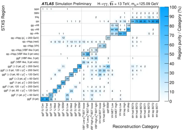
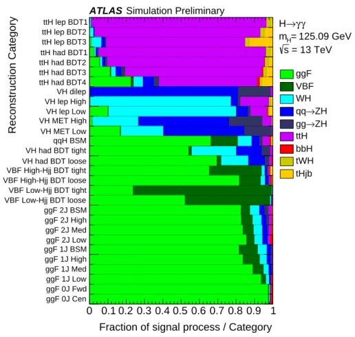
A summary of the definitions of all categories is provided in Table 3. Figure 4 shows the compositon of signal events for each category in terms of different simplified template cross section regions, while Figure 5 shows the composition of signal events for each category in terms of different production modes.

More information about the signal efficiencies times acceptance, composition of signal events, effective

signal mass resolution, and number of signal and background events for each category can be found in

Tables 9, 10 and 11 in the appendix.

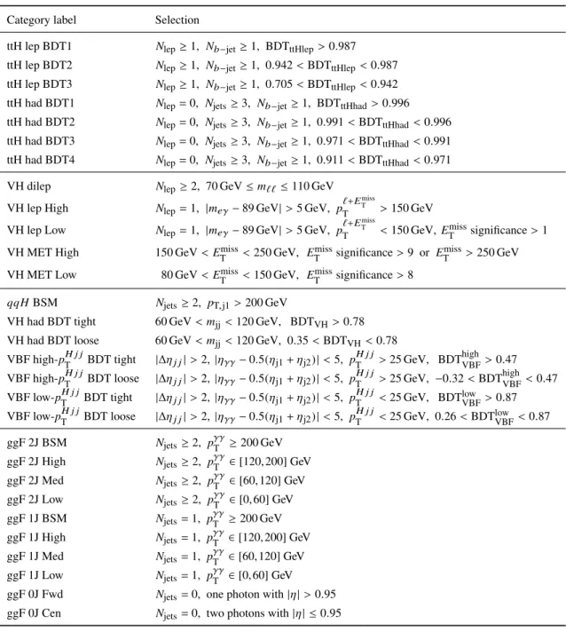
Category label Selection

ttH lep BDT1 N

≥ 1, N

≥ 1, BDT

> 0.987 ttH lep BDT2 N

≥ 1, N

≥ 1, 0.942 < BDT

< 0.987 ttH lep BDT3 N

≥ 1, N

≥ 1, 0.705 < BDT

< 0.942 ttH had BDT1 N

= 0, N

≥ 3, N

≥ 1, BDT

> 0.996 ttH had BDT2 N

= 0, N

≥ 3, N

≥ 1, 0.991 < BDT

< 0.996 ttH had BDT3 N

= 0, N

≥ 3, N

≥ 1, 0.971 < BDT

< 0.991 ttH had BDT4 N

= 0, N

≥ 3, N

≥ 1, 0.911 < BDT

< 0.971 VH dilep N

≥ 2, 70 GeV ≤ m

≤ 110 GeV

VH lep High N

= 1, | m

− 89 GeV | > 5 GeV, p

> 150 GeV

VH lep Low N

= 1, | m

− 89 GeV | > 5 GeV, p

< 150 GeV, E

significance > 1 VH MET High 150 GeV < E

< 250 GeV, E

significance > 9 or E

> 250 GeV VH MET Low 80 GeV < E

< 150 GeV, E

significance > 8

qqH BSM N

≥ 2, p

> 200 GeV

VH had BDT tight 60 GeV < m

< 120 GeV, BDT

> 0.78 VH had BDT loose 60 GeV < m

< 120 GeV, 0.35 < BDT

< 0.78

VBF high-p

BDT tight |∆η

| > 2, | η

− 0.5(η

+ η

)| < 5, p

> 25 GeV, BDT

> 0.47 VBF high-p

BDT loose | ∆η

| > 2, | η

− 0.5(η

+ η

) | < 5, p

> 25 GeV, − 0.32 < BDT

< 0.47 VBF low-p

BDT tight | ∆η

| > 2, | η

− 0.5(η

+ η

) | < 5, p

< 25 GeV, BDT

> 0.87 VBF low-p

BDT loose | ∆η

| > 2, | η

− 0.5(η

+ η

) | < 5, p

< 25 GeV, 0.26 < BDT

< 0.87 ggF 2J BSM N

≥ 2, p

≥ 200 GeV

ggF 2J High N

≥ 2, p

∈ [120, 200] GeV ggF 2J Med N

≥ 2, p

∈ [60,120] GeV ggF 2J Low N

≥ 2, p

∈ [0, 60] GeV ggF 1J BSM N

= 1, p

≥ 200 GeV ggF 1J High N

= 1, p

∈ [120,200] GeV ggF 1J Med N

= 1, p

∈ [60, 120] GeV ggF 1J Low N

= 1, p

∈ [0, 60] GeV ggF 0J Fwd N

= 0, one photon with | η | > 0.95 ggF 0J Cen N

= 0, two photons with | η | ≤ 0.95

Table 3: Summary of the 29 event reconstruction categories for the measurement of production mode cross sections

and simplified template cross sections. Each category targets a particle-level kinematic region that is reflected

in the category label. Each event is assigned to the first category whose requirements are satisfied, using the

descending order given in the table. As a result, the event populations of categories are mutually exclusive. Note

that the categories are separated by horizontal lines based on the definitions of the stage-0 simplified template cross

sections: top, V H leptonic, qq

→ Hqq

(VBF + V H ), and ggF. Though some of the non-t tH ¯ category names have

changed, the definition of those categories is the same as in Ref. [7]. N

denotes the number of selected electrons

and muons, N

the number of selected jets, and N

the number of b-tagged jets. Other variables are defined in

the text.

91 90 38 3 24 1 3 8 2 5

5 5 51 1 25 5 12 1 2

1 76 2 24 6 1 10 8 8 2 4 1

70 1 10 1 2 4 3 3

69 3 4

3 34 2 4 2 1 1

8 56 1 3 9 4 26 9 3 6 3 1

10 71 2 1 11 4 25 30 10 3 8 4 1

11 79 2 3 8 5 14 43 11 7 4 2

26 14 4 5 1

1 4 3 18 30 3 1

1 36 68 3 8

2 4 5 18

3 2 2 2 20 35 3 1

4 8 10 2 7 10 11 9 10 4 6 4 5 3 5 3 1

12 23 3 2

1 1 22 25 69 77 5 2

44 49 6 4 81 2

15 18 1 1 18

1 1 1 2 1 1 4 5 9 16 1 54 75 86 91 76 90 95

2 2 1 6 4 2 1 13 5 1

1 1 2 2 3 2 2 2

1 1 1 1 1

ggF 0J Cen ggF 0J Fwd ggF 1J Low ggF 1J Med ggF 1J High ggF 1J BSM ggF 2J Low ggF 2J Med ggF 2J High ggF 2J BSM BDT looseHjj TVBF Low-p BDT tightHjj TVBF Low-p BDT looseHjj TVBF High-p BDT tightHjj TVBF High-p VH had BDT loose VH had BDT tight qqH BSM VH MET Low VH MET High VH lep Low VH lep High VH dilep ttH had BDT4 ttH had BDT3 ttH had BDT2 ttH had BDT1 ttH lep BDT3 ttH lep BDT2 ttH lep BDT1

Reconstruction Category

ggF (0-jet) < 60 GeV)

H

ggF (1-jet, pT

< 120 GeV)

H

pT

ggF (1-jet, 60 ≤

< 200 GeV)

H

pT

ggF (1-jet, 120 ≤

200 GeV)

H≥ ggF (1-jet, pT

< 60 GeV)

H

2-jet, pT

ggF (≥

< 120 GeV)

H

pT

2-jet, 60 ≤ ggF (≥

< 200 GeV)

H

pT

2-jet, 120 ≤ ggF (≥

200 GeV)

H≥ 2-jet, pT

ggF (≥

ggF (VBF-like, 3-jet veto) ggF (VBF-like, 3-jet) Hqq (VBF-like 3-jet veto) qq→

Hqq (VBF-like 3-jet) qq→

Hqq (VH) qq→

Hqq (rest) qq→

200 GeV)

j≥ Hqq (pT

qq→

Hlν qq→

Hll qq→

→Hll gg

ttH tHq tWH bbH

STXS Region

0 10 20 30 40 50 60 70 80 90 100 Simulation Preliminary

ATLAS H → γ γ , s = 13 TeV, m

= 125.09 GeV

Region purity / Category (%)

Figure 4: The expected composition of signal events, as classified by the particle-level regions (rows) of the stage-1 simplified template cross sections (STXS), in each reconstruction category (columns). Some stage-1 regions are merged in cases where the data set lacks the sensitivity to resolve them. For each reconstruction category, the target particle-level categories are indicated with a box. The gray horizontal and vertical lines delimit stage-0 STXS regions and their corresponding reconstruction categories. Numbers in each column add up to 100%. Entries smaller than 1% are suppressed.

8.2 Production mode measurements

The global signal strength, production mode cross sections and simplified template cross sections are extracted using simultaneous fits to the diphoton invariant mass distribution in the 29 categories, with the extended likelihood functions described in Section 6.3.

8.2.1 Observed Data

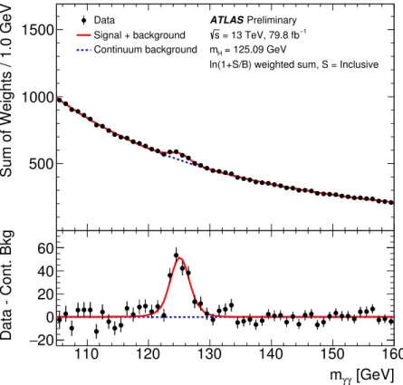
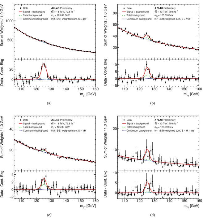
Figure 6 and Figure 7 show the weighted diphoton invariant mass distributions observed in 79.8 fb ⁻¹ of

13 TeV data using all analysis categories. Events are weighted by ln(1+S 90 / B 90 ), where S 90 (B 90 ) for each

category is the expected signal (background) in the smallest m γγ window containing 90% of the expected

signal. In Figure 6, the signal is the sum of all Higgs production modes. In Figure 7 (a) - (d), the signal

is ggF, VBF, V H , and top-associated production, respectively, while the other Higgs boson production

modes are included in the background. In both figures, the solid red curve shows the fitted signal-plus-

background model with the Higgs boson mass constrained to 125.09 ± 0.24 GeV. This constraint is

consistent with the observed mass peak position. The fit is performed in all analysis categories for the

global signal strength, assuming the relative ratios of different production modes are as predicted by the

0 0.1 0.2 0.3 0.4 0.5 0.6 0.7 0.8 0.9 1 Fraction of signal process / Category

ggF 0J Cen ggF 0J Fwd ggF 1J Low ggF 1J Med ggF 1J High ggF 1J BSM ggF 2J Low ggF 2J Med ggF 2J High ggF 2J BSM VBF Low-Hjj BDT loose VBF Low-Hjj BDT tight VBF High-Hjj BDT loose VBF High-Hjj BDT tight VH had BDT loose VH had BDT tight qqH BSM VH MET Low VH MET High VH lep Low VH lep High VH dilep ttH had BDT4 ttH had BDT3 ttH had BDT2 ttH had BDT1 ttH lep BDT3 ttH lep BDT2 ttH lep BDT1

Reconstruction Category

ggF VBF WH

→ ZH qq

→ ZH gg ttH bbH tWH tHjb Simulation Preliminary

ATLAS

γ γ

→ H

125.09 GeV

H

= m

= 13 TeV s

Figure 5: The expected composition of signal events, based on production mode, of each reconstruction category.

SM. The non-resonant background component is shown with the dotted blue curve. In Figure 7, the total background component is shown with the dashed green curve. Both the signal-plus-background and background-only curves shown here are obtained from the weighted sum of the individual curves in each analysis category.

8.2.2 Production mode cross sections

A global signal strength µ is measured for the inclusive Higgs boson production, assuming the ratios of different production modes are the same as in the SM prediction within the assigned theoretical systematic uncertainties. µ is found to be

µ = 1.06 ^+0.14 _{− 0.12} = 1.06 ± 0.08 (stat.) ^+0.08 _{− 0.07} (exp.) ^+0.07 _{− 0.06} (theo.) ,

which is consistent with the SM expectation ( µ = 1). The global signal strength measurement is dominated by the systematic uncertainty, for which the experimental uncertainty and theoretical uncertainty have similar importance.

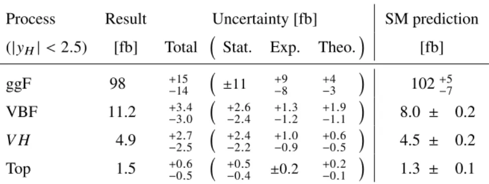
The production mode cross sections are evaluated in a region with Higgs-boson rapidity | y H | < 2 . 5.

σ _top , denoted as the sum of the t tH ¯ , tHq, and tHW production mode cross sections, is fitted under the

assumption that their relative ratios are as predicted by the SM. Similarly, the V H production mode cross

110 120 130 140 150 160 500

1000 1500

Sum of Weights / 1.0 GeV

Data

Signal + background Continuum background

Preliminary ATLAS

1

= 13 TeV, 79.8 fb

s

= 125.09 GeV m

ln(1+S/B) weighted sum, S = Inclusive

110 120 130 140 150 160

[GeV]

γ

m γ

20

− 0 20 40 60

Data - Cont. Bkg

Figure 6: Weighted diphoton invariant mass spectrum in all the analysis categories observed in 79.8 fb

of 13 TeV

data. Events are weighted by ln(1+S

/B

), where S

(B

) for each category is the expected signal (background)

in the smallest m

window containing 90% of the expected signal. The signal is the sum of all Higgs production

modes. The error bars represent 68% confidence intervals of the weighted sums. The solid red curve shows the

fitted signal-plus-background model with the Higgs boson mass constrained to 125.09 ± 0.24 GeV. The fit is done

in all the analysis categories for the global signal strength, assuming the relative ratios of different production modes

are as predicted by the SM. The non-resonant background component of the fitted signal-plus-background model

is shown with the dotted blue curve. Both the signal-plus-background and background-only curves shown here are

obtained from the weighted sum of the individual curves in each analysis category. The lower panel shows the

residuals between the data and the non-resonant background component.