Combined measurements of the mass and signal strength of the Higgs-like boson with the ATLAS detector using up to 25 fb − 1 of proton-proton

A TLAS-CONF-2013-014 06 Mar ch 2013

ATLAS NOTE

ATLAS-CONF-2013-014

March 5, 2013

Combined measurements of the mass and signal strength of the Higgs-like boson with the ATLAS detector using up to 25 fb ^{− 1} of proton-proton

collision data

The ATLAS Collaboration

Abstract

An update is presented of the measurement of the properties of the newly discovered boson using the the full pp collision data sample recorded by the ATLAS experiment at the LHC for the channels H → γγ and H → ZZ

→ 4ℓ, corresponding to integrated lumi- nosities of about 4.8 fb

at √

s = 7 TeV and 20.7 fb

at √

s = 8 TeV. The combined mass measurement derived from the H → γγ and H → ZZ

→ 4ℓ channels is m

= 125.5 ± 0.2 (stat)

(sys) GeV.

The combination of all studied final states, including the H → ττ and H → b b ¯ channels using data corresponding to integrated luminosities of about 4.8 fb

at √ s = 7 TeV and 13 fb

at √

s = 8 TeV and the H → WW

→ ℓνℓν channel using data corresponding to an integrated luminosity of 13 fb

at √

s = 8 TeV, is reported in terms of the combined signal strength (µ) and production and decay mode specific signal strengths. The combined signal strength is determined to be µ = 1.43 ± 0.16 (stat) ± 0.14 (sys) at a mass of 125.5 GeV.

c Copyright 2013 CERN for the benefit of the ATLAS Collaboration.

Reproduction of this article or parts of it is allowed as specified in the CC-BY-3.0 license.

1 Introduction

The observation of a new particle in the search for the Standard Model (SM) Higgs boson at the LHC, reported by the ATLAS [1] and CMS [2] Collaborations, is a milestone in the quest to understand elec- troweak symmetry breaking [3–5]. In Refs. [1, 6] the ATLAS Collaboration reported first measurements of the mass of this particle and its coupling properties. An update of the combined signal strength value for the channels H → WW

→ ℓνℓν, H → ττ and H → b b ¯ has been reported in Ref. [7]. Recently the mass and signal strength measurements for H → γγ and H → ZZ

→ 4ℓ have been updated using about 13 fb

at √

s = 8 TeV [8]. This document presents an update of the combined measurements of the mass and signal strength of the observed new particle including the updated analyses for H → γγ [9] and H → ZZ

→ 4ℓ [10] using about 4.8 fb

of pp collision data at √

s = 7 TeV and 20.7 fb

at √

s = 8 TeV.

The results are based on the same statistical model as in Refs. [1, 6]. The aspects of the individual channels relevant for these measurements are briefly summarized in Section 2. The statistical procedure and the treatment of systematic uncertainties are outlined in Section 3. The measurement of the mass, obtained from the H → γγ and H → ZZ

→ 4ℓ channels, is described in Section 4. Finally in Section 5 the measured yields are analysed in terms of the signal strengths, for different production and decay modes and for their combination.

2 Individual channels

For the H → γγ and H → ZZ

→ 4ℓ channels, the updated analyses based on the full 2011 and 2012 datasets of 4.8 fb

at √

s = 7 TeV and 20.7 fb

at √

s = 8 TeV as presented in Refs. [9, 10] are used.

For the H → ττ and H → b b ¯ channels, the analyses [11, 12] are applied to the full 2011 data sample at

√ s = 7 TeV and a subsample of the 2012 data of 13 fb

at √

s = 8 TeV. For the H → WW

→ ℓνℓν final state, the results in Ref. [13], based on 13 fb

of 2012 data, are considered here. The different final states and channel categories considered in this study are summarized in Table 1.

3 Statistical procedure

The statistical modelling of the data is described in Refs. [14–17].

The likelihood function of the observed data is parametrized in terms of scale factors for the cross section σ

of each SM Higgs production mode, the branching ratios B

of the SM Higgs boson decays, and the mass of the Higgs boson m

. For each production mode i, a signal strength factor µ

defined as µ

= σ

/σ

is introduced. Similarly, for each decay final state f , a factor µ

= B

/B

is introduced. For each analysis category (k) the number of signal events (n

) is parametrized as:

n

=



 

 

  X

i

µ

σ

× A

× ε



 

 

  × µ

× B

× L

, (1)

where A represents the detector acceptance, ε the reconstruction efficiency and L the integrated lumi-

nosity. The number of signal events expected from each combination of production and decay modes

is scaled by the corresponding product µ

µ

, with no change to the distribution of kinematic or other

properties. This parametrization generalizes the dependency of the signal yields on the production cross

sections and decay branching fractions, allowing for a coherent variation across several channels. This

approach is also general in the sense that it is not restricted by any relationship between production cross

sections and branching ratios. For instance, it is possible to force the production cross section σ

= 0

while maintaining a non-zero branching ratio B

.

In the simplest cases, the product µ

µ

can also be represented by a single signal strength parameter µ

, where j is an index representing both the production and decay indices i and f . For example, the global signal strength µ scales the total number of events from the combination of all production and decay modes relative to their SM values, such that µ = 0 corresponds to the background-only hypothesis and µ = 1 corresponds to the SM Higgs boson signal in addition to the background.

The combined results presented in this note assume that all measurements are compatible with a sin- gle resonance hypothesis. The masses measured from the two high resolution H → γγ and H → ZZ

→ 4ℓ channels, denoted by m

and m

, are compared for compatibility by defining ∆m

≡ m

− m

. The chosen likelihood is a function of a vector of signal strength factors µ, the masses m

(the combined mass), m

and m

and nuisance parameters θ. Hypothesis testing and confidence intervals are based on the profile likelihood ratio [18]. The parameters of interest depend on the test in question, while the remaining parameters are profiled. As indicated in the sections below, the mass parameter m

may be fixed, be an explicit parameter of interest, or be profiled.

Table 1: Summary of the individual channels entering the combined results presented here. In channels sensitive to associated production of the Higgs boson, V indicates a W or Z boson. The symbols ⊗ and ⊕ represent direct products and sums over sets of selection requirements, respectively. The abbreviations listed here are described in the corresponding Refs. reported in the last column. For the determination of the µ

to µ

correlation reported in Section 5, H → ZZ

→ 4ℓ results including VBF and V H categories were used.

Higgs Boson Subsequent

Sub-Channels

R L dt

Decay Decay [fb

] Ref.

2011 √

s =7 TeV

H → ZZ

4ℓ { 4e, 2e2µ, 2µ2e, 4µ } 4.6 [10]

H → γγ – 10 categories

4.8 [9]

{ p

⊗ η

⊗ conversion } ⊕ { 2-jet VBF } H → ττ

τ

τ

{ eµ } ⊗ { 0-jet } ⊕ { ℓℓ } ⊗ { 1-jet, 2-jet, p

> 100 GeV, V H } 4.6

τ

τ

{ e, µ } ⊗ { 0-jet, 1-jet, p

> 100 GeV, 2-jet } 4.6 [11]

τ

τ

{ 1-jet, 2-jet } 4.6

V H → Vbb

Z → νν E

∈ { 120 − 160, 160 − 200, ≥ 200 GeV } ⊗ { 2-jet, 3-jet } 4.6

W → ℓν p

∈ { < 50, 50 − 100, 100 − 150, 150 − 200, ≥ 200 GeV } 4.7 [12]

Z → ℓℓ p

∈ { < 50, 50 − 100, 100 − 150, 150 − 200, ≥ 200 GeV } 4.7 2012 √

s =8 TeV

H → ZZ

4ℓ { 4e, 2e2µ, 2µ2e, 4µ } 20.7 [10]

H → γγ – 14 categories

20.7 [9]

{ p

⊗ η

⊗ conversion } ⊕ { 2-jet VBF } ⊕ { ℓ-tag, E

-tag, 2-jet VH }

H → WW

eνµν { eµ, µe } ⊗ { 0-jet, 1-jet } 13 [13]

H → ττ

τ

τ

{ ℓℓ } ⊗ { 1-jet, 2-jet, p

> 100 GeV, V H } 13

τ

τ

{ e, µ } ⊗ { 0-jet, 1-jet, p

> 100 GeV, 2-jet } 13 [11]

τ

τ

{ 1-jet, 2-jet } 13

V H → Vbb

Z → νν E

∈ { 120 − 160, 160 − 200, ≥ 200 GeV } ⊗ { 2-jet, 3-jet } 13

W → ℓν p

∈ { < 50, 50 − 100, 100 − 150, 150 − 200, ≥ 200 GeV } 13 [12]

Z → ℓℓ p

∈ { < 50, 50 − 100, 100 − 150, 150 − 200, ≥ 200 GeV } 13

Hypothesized values of µ are tested with the statistic:

Λ(µ) = L µ, θ(µ) ˆˆ

L( ˆ µ, θ) ˆ (2)

where the single circumflex (e.g. ˆ µ, ˆ θ) denotes the unconditional maximum likelihood estimate of a parameter and the double circumflex (e.g. θ(µ)) denotes the conditional maximum likelihood estimate ˆˆ (e.g. of θ) for given fixed values of µ. This test statistic extracts the information on the parameters of interest from the full likelihood function.

Hypothesized values of m

are tested with a similarly defined profile likelihood ratio Λ(m

) = L m

, µ ˆˆ

(m

) , µ ˆˆ

(m

) , θ(m ˆˆ

)

L( ˆ m

, µ ˆ

, µ ˆ

, θ) ˆ . (3) Asymptotically, the test statistic − 2 ln Λ(µ, m

) for several parameters of interest µ and m

is dis- tributed as a χ

distribution with n degrees of freedom, where n is the sum of the dimensionality of the vectors µ and m

. In particular, the 100(1 − α)% confidence level (CL) contours are defined by

− 2 ln Λ(µ, m

) < k

, where k

satisfies P(χ

> k

) = α. For two degrees of freedom the 68% and 95% CL contours are given by − 2 ln Λ(µ, m

) = 2.3 and 6.0, respectively.

The treatment of systematic uncertainties and of their correlations is described in detail in Ref. [14].

Mass scale related systematic uncertainties are described in Ref. [8]. Systematic uncertainties on observ- ables are handled by introducing nuisance parameters with a probability density function (pdf) associated with the estimate of the corresponding effect. These nuisance parameters, in particular those represent- ing instrumental uncertainties or background estimates, are often assessed from auxiliary measurements, such as control regions, sidebands, or dedicated calibration measurements. Their pdfs are described ei- ther by a Gaussian or alternatively by a log-normal distribution to avoid the truncation of a pdf bounded to a restricted range, which should be an accurate description for most cases. In cases where the un- certainty is related to a number of events (e.g. from Monte Carlo or data control samples) the Poisson function is used. For nuisance parameters unconstrained by considerations or measurements, a pdf is not a priori defined. This is typically the case for theory uncertainties on the prediction of production cross sections or branching ratios [20, 21], for which log-normal distributions are chosen [15]. Another exam- ple is the use of rectangular pdfs for the systematic mass scale uncertainties as discussed in Ref. [8]. The rectangular pdfs give a flat a priori likelihood in the range of the ± 1σ Gaussian uncertainty intervals.

4 Mass measurement

The mass of the newly discovered boson can be measured precisely in the high mass resolution channels H → γγ and H → ZZ

→ 4ℓ. A mass of m

= 126.8 ± 0.2 (stat) ± 0.7 (sys) GeV is found in the H → γγ channel [9] and a mass of m

= 124.3

(stat)

(sys) GeV in the H → ZZ

→ 4ℓ channel [10]. In this section an update of the combined mass between these two channels and their compatibility is reported.

The same statistical methods as described in Ref. [8] are used.

4.1 Combined mass determinations from the H → γγ and H → ZZ

→ 4ℓ channels

An estimate of the mass of the Higgs-like boson, combining the H → γγ and H → ZZ

→ 4ℓ channels, is based on the profile likelihood ratio Λ(m

) described in Eqn. 3. This method allows the signal strength

1

Here Λ is used for the profile likelihood ratio to avoid confusion with the parameter λ used in Higgs boson coupling scale

factor benchmarks [19].

to vary independently between the two channels (treating both signal strengths as nuisance parameters), while the ratios of the cross sections of the different production modes within each channel are fixed to the SM values. The leading source of systematic uncertainty in the mass estimate comes from the mass scale systematic uncertainties [8–10]. Figure 1 shows the profile likelihood ratio as a function of m

for the H → γγ and H → ZZ

→ 4ℓ channels and their combination. The combined mass is measured to be

m

= 125.5 ± 0.2 (stat)

(sys) GeV . (4)

[GeV]

mH

121 122 123 124 125 126 127 128 129

Λ-2ln

0 1 2 3 4 5 6 7

σ 1

σ 2

Preliminary ATLAS

Ldt = 4.6-4.8 fb-1

∫

= 7 TeV:

s

Ldt = 20.7 fb-1

∫

= 8 TeV:

s

Combined (stat+sys) Combined (stat only)

γ γ

→ H

l

→ 4 ZZ(*)

→ H

Figure 1: The profile likelihood ratio − 2 ln Λ(m

) as a function of m

for the H → γγ and H → ZZ

→ 4ℓ channels and their combination, obtained by allowing the signal strengths µ

and µ

to vary indepen- dently. The dashed line shows the statistical component of the mass measurement uncertainty.

4.2 Consistency of the mass determinations from H → γγ and H → ZZ

→ 4ℓ

For the previous combination reported in Ref. [8] the compatibility of the two mass measurements was 0.8% (2.7σ). To assess the consistency of the updated measurements, a likelihood function in which the mass parameters m

and m

vary independently is considered first. Figure 2(a) shows likelihood contours in m

and m

around the two best-fit mass values and the line ˆ m

= m ˆ

= m ˆ

. The largest correlation between the measurements is the overall e/γ energy scale from the Z → e

e

based calibration. The mass consistency between the muon and electron final states in the H → ZZ

→ 4ℓ channel causes a ∼ 0.8σ adjustment in the overall e/γ energy scale which induces an approximate 350 MeV downward shift of m

in the combination, with respect to the value measured from this channel alone.

To quantify the consistency between the measured m

and m

values, a likelihood function is con- sidered for the mass difference ∆m

= m

− m

, with the average mass m

profiled in the fit:

Λ(∆m

) = L ∆m

, µ ˆˆ

(∆m

) , µ ˆˆ

(∆m

) , m ˆˆ

(∆m

) , θ(∆m ˆˆ

)

L( ˆ ∆m

, µ ˆ

, µ ˆ

, m ˆ

, θ) ˆ . (5)

This allows the hypothesis ∆m

= 0 to be tested. The signal strengths µ

and µ

are again treated

as independent nuisance parameters. The likelihood is shown in Figure 2(b) as a function of the mass

[GeV]

γ

mγ

122 123 124 125 126 127 128 129

[GeV]4lm

122 123 124 125 126 127 128

129 ATLAS Preliminary

Ldt = 4.6-4.8 fb-1

∫

= 7 TeV:

s

Ldt = 20.7 fb-1

∫

= 8 TeV:

s Best fit 68% CL 95% CL 99.7% CL

H=0

∆m

(a)

[GeV]

-m4l γ

mγ

-1 0 1 2 3 4 5

Λ-2ln

0 2 4 6 8 10

σ 1

σ 2

σ 3

Λ(0) -2ln

Preliminary ATLAS

Ldt = 4.6-4.8 fb-1

∫

= 7 TeV:

s

Ldt = 20.7 fb-1

∫

= 8 TeV:

s

(b)

Figure 2: (a) Likelihood contours as a function of m

and m

. (b) Likelihood as a function of the mass difference, ∆m

= m

− m

, profiling over the common mass m

. In both cases the signal strength parameters µ

and µ

are allowed to vary independently. In (a) the masses are considered as two independent parameters of interest (2-dimensional contours) while in (b) only one parameter of interest, the mass difference, is considered (1-dimensional variation of the likelihood).

difference. The estimated H → γγ and H → ZZ

→ 4ℓ mass difference is

∆ m ˆ

= m ˆ

− m ˆ

= 2.3

(stat) ± 0.6 (sys) GeV , (6) where the 68% CL errors are computed with the asymptotic approximation. The mass difference is re- duced with respect to the one reported in Ref. [8] by about 700 MeV. This reduction is driven by changes in the individual measurements reported in Refs. [9, 10] where the compatibility with the previously measured values is discussed.

From the value of the likelihood evaluated at ∆m

= 0, indicated in Figure 2(b), the probability for a single Higgs-like boson to produce a value of the Λ(∆m

) test statistic disfavoring the ∆m

= 0 hypothesis by more than observed in the data is found to be at the level of 1.2% (2.5σ) using the asymptotic approximation assumption, and 1.5% (2.4σ) using Monte Carlo ensemble tests.

Further checks, assuming the SM signal strengths for H → γγ and H → ZZ

→ 4ℓ, or constraining the ensemble of pseudo-experiments to the observed signal strengths, yield similar probabilities, since µ and m

are largely uncorrelated.

The significance of the mass difference is also tested using rectangular pdfs for the systematic energy scale uncertainties coming from the Z → ee calibration method, the imperfect knowledge of the material upstream of the electromagnetic calorimeter and the energy scale of the presampler detector. The rectan- gular pdfs give a flat a priori likelihood in the range of the ± 1σ Gaussian uncertainty intervals for these three sources of systematic uncertainties and a zero probability outside the ± 1σ range. The use of such a pdf model leads to a coherent shift within the allowed parameter range to values which reduce the mass difference. The overall mass difference is thus decreased by an amount corresponding to the linear sum of the individual Gaussian errors for these three sources of systematic uncertainties. With this treatment of these energy scale systematic uncertainties the probability for a single Higgs-like boson to produce a

2

Here 2-sided probabilities are used as both cases, m

> m

and m

< m

, are considered.

value of the Λ(∆m

) test statistic disfavoring the ∆m

= 0 hypothesis by more than observed in the data is found to be 8%.

5 Signal production strength in individual decay modes

This section focuses on the global signal strength parameter µ, as well as the strength parameters µ

for the individual channels characterized by a production mode i and decay mode f , for a fixed mass m

. Hypothesized values of µ and µ

are tested with the statistic Λ(µ) as defined in Eqn. 2. This test statistic extracts the information on the parameters of interest from the full likelihood function.

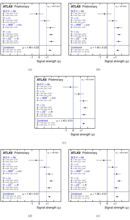
The best-fit signal strength parameter µ is a convenient observable to test the compatibility of the data with the background-only hypothesis (µ = 0) and the SM Higgs hypothesis (µ = 1). The best-fit values of the signal strength parameter for each channel independently and for the combination are given in Fig. 3 and Table 2 for the measured combined mass m

= 125.5 GeV. Checks allowing the Higgs boson mass hypothesis to float, using it as an additional nuisance parameter in the measurements of µ, and thus taking into account the experimental uncertainty on its estimate, were performed and no significant deviations from the results presented herein were observed.

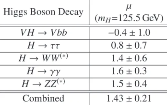
The observed yield corresponds to a measured signal strength of 1.43 ± 0.16 (stat) ± 0.14 (sys) for m

= 125.5 GeV with all channels combined. This combined signal strength is consistent with the SM Higgs boson hypothesis µ = 1 at the 3% level. Alternatively, the consistency with the SM Higgs boson hypothesis is also tested using rectangular pdfs for the dominant theory systematic uncertainties from gg → H QCD scale and PDF variations following the recommendations in Refs. [20, 21]. With this treatment the consistency of the observed signal strength with the SM hypothesis is increased to ∼ 11%.

A compatibility test between the signal strengths of the five channels and the Standard Model expectation of unity for all channels gives a probability of about 8%. The compatibility between the combined best- fit signal strength ˆ µ and the best-fit signal strengths of the five channels is 32%. The dependence of the combined value of ˆ µ on the assumed m

has been investigated and is relatively weak: changing the mass hypothesis between 124.5 and 126.5 GeV changes the value of ˆ µ by about 4%.

Table 2: Summary of the best-fit values and uncertainties for the signal strength µ for the individual channels and their combination for a Higgs boson mass of 125.5 GeV.

Higgs Boson Decay µ

(m

=125.5 GeV) V H → Vbb − 0.4 ± 1.0

H → ττ 0.8 ± 0.7

H → WW

1.4 ± 0.6

H → γγ 1.6 ± 0.3

H → ZZ

1.5 ± 0.4

Combined 1.43 ± 0.21

In order to test which values of signal strength and Higgs mass are simultaneously consistent with the data for the H → γγ and H → ZZ

→ 4ℓ channels, the profile likelihood ratio Λ(µ, m

) is used. Asymp- totically, the test statistic − 2 ln Λ(µ, m

) is distributed as a χ

distribution with two degrees of freedom.

The resulting 68% and 95% CL contours are shown in Fig. 4.

In addition to the signal strength in different decay modes, the signal strengths of different Higgs

production processes contributing to the same final state are determined. Such a separation avoids model

assumptions needed for a consistent parametrization of both production and decay mode modifications in

terms of Higgs boson couplings. In the SM, the production cross sections are completely fixed once m

µ ) Signal strength ( -1 0 +1

→ 4l ZZ(*)

→ H

γ γ H →

ν νl

→ l WW(*)

→ H

τ τ

→ H

→ bb W,Z H

Ldt = 4.6 - 4.8 fb-1

∫

= 7 TeV:

s

Ldt = 13 - 20.7 fb-1

∫

= 8 TeV:

s

Ldt = 4.6 fb-1

∫

= 7 TeV:

s

Ldt = 20.7 fb-1

∫

= 8 TeV:

s

Ldt = 4.8 fb-1

∫

= 7 TeV:

s

Ldt = 20.7 fb-1

∫

= 8 TeV:

s

Ldt = 13 fb-1

∫

= 8 TeV:

s

Ldt = 4.6 fb-1

∫

= 7 TeV:

s

Ldt = 13 fb-1

∫

= 8 TeV:

s

Ldt = 4.7 fb-1

∫

= 7 TeV:

s

Ldt = 13 fb-1

∫

= 8 TeV:

s

= 125.5 GeV mH

0.21

± = 1.43 µ

ATLAS Preliminary

Figure 3: Measurements of the signal strength parameter µ for m

=125.5 GeV for the individual chan- nels and for their combination.

[GeV]

mH

122 123 124 125 126 127 128 129

)µSignal strength (

0 0.5 1 1.5 2 2.5 3 3.5

4 ATLAS Preliminary

Ldt = 4.6-4.8 fb-1

∫

= 7 TeV:

s

Ldt = 20.7 fb-1

∫

= 8 TeV:

s

Combined γ γ

→ H

l

→ 4 ZZ(*)

→ H Best fit 68% CL 95% CL

Figure 4: Confidence level intervals in the (µ, m

) plane for the H → ZZ

→ 4ℓ and H → γγ channels and their combination, including all systematic uncertainties. The markers indicate the maximum likelihood estimates ( ˆ µ, m ˆ

) in the corresponding channels.

is specified. The best-fit value for the global signal strength factor µ does not give any direct information on the relative contributions from different production modes. Furthermore, fixing the ratios of the production cross sections to the ratios predicted by the SM may conceal tension between the data and the SM.

Since several Higgs boson production modes are available at the LHC, results shown in two dimen-

sional plots require either some µ

to be fixed or several µ

to be related. No direct ttH production has

been observed yet, hence µ

and the very small contribution of µ

have been grouped together as they

scale dominantly with the ttH coupling in the SM and are denoted by the common parameter µ

.

B/B SM ggF+ttH ×

µ

-2 -1 0 1 2 3 4 5 6 7

SM B/B × VBF+VH µ

-4 -2 0 2 4 6 8 10

Standard Model Best fit 68% CL 95% CL γ

γ

→ H

→ 4l ZZ(*)

→ H

τ τ

→ H

Preliminary ATLAS

Ldt = 4.6-4.8 fb

∫

= 7 TeV:

s

Ldt = 13-20.7 fb

∫

= 8 TeV:

s

= 125.5 GeV mH

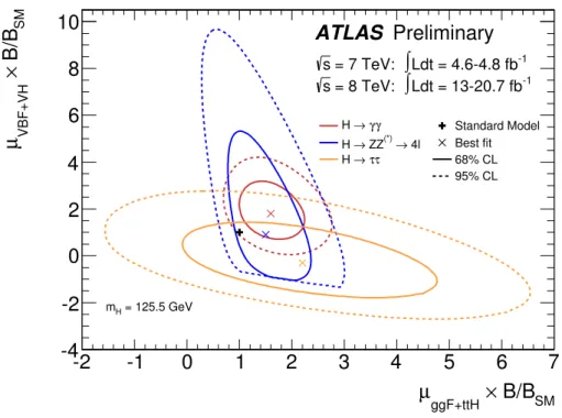
Figure 5: Likelihood contours for the H → γγ, H → ZZ

→ 4ℓ and H → ττ channels in the (µ

, µ

) plane for a Higgs boson mass hypothesis of m

= 125.5 GeV. Both µ

and µ

are modified by the branching ratio factor B/B

, which can be different for the different final states. The quantity µ

(µ

) is a common scale factor for the gluon fusion and t¯ tH (VBF and V H ) production cross sections. The best-fit to the data ( × ) and 68% (full) and 95% (dashed) CL contours are also indicated, as well as the SM expectation (+).

Similarly, µ

and µ

have been grouped together as they scale with the W H/ZH gauge coupling in the SM and are denoted by the common parameter µ

. The resulting contours for the H → γγ, H → ZZ

→ 4ℓ and H → ττ channels, each using analysis categories optimized for the measurement of VBF Higgs production, are shown in Fig. 5 for m

=125.5 GeV.

The factors µ

are not constrained to be positive in order to illustrate a deficit of events from the corresponding production process. As described in Ref. [14], while the signal strengths may be negative, the total number of signal plus background expected events must remain positive. This restriction is responsible for the sharp cutoff in the H → ZZ

→ 4ℓ contour shown in Fig. 5. It should be noted that each contour refers to a different branching fraction B/B

, hence a direct comparison of the contours from different final states is not possible. It should be noted that the factors µ

, the ratio of the branching ratio in a given final state f to the SM one may have different values for different decay modes, hence a direct comparison of the results among different final states is not possible. Such comparisons need consistent coupling modifications in the initial and final state. It is possible, however, to use ratios to eliminate the dependence on the branching fractions and illustrate the relative discriminating power between ggH + ttH and V BF + V H, as well as the compatibility of the measurements across channels.

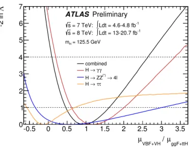
The likelihood as a function of the ratio µ

/µ

is shown for the H → γγ, H → ZZ

→ 4ℓ and

H → ττ channels and their combination in Fig. 6. The measurements in the three channels as well as

the observed combined ratio of µ

/µ

= 0.9

are compatible with the SM expectation of

unity.

ggF+ttH

µ

VBF+VH

/ µ

-0.5 0 0.5 1 1.5 2 2.5 3 3.5

Λ -2 ln

0 1 2 3 4 5 6 7

combined γ γ

→ H

→ 4l ZZ(*)

→ H

τ τ

→ H

Preliminary ATLAS

Ldt = 4.6-4.8 fb-1

∫

= 7 TeV:

s

Ldt = 13-20.7 fb-1

∫

= 8 TeV:

s

= 125.5 GeV mH

Figure 6: Likelihood curves for the ratio µ

/µ

from the H → γγ, H → ZZ

→ 4ℓ and H → ττ channels, and their combination, for a Higgs boson mass hypothesis of m

= 125.5 GeV. The branch- ing ratios, and possible non-SM effects affecting them, cancel in the ratio µ

/µ

, hence the different measurements from all three channels can be compared and combined.

6 Conclusion

An update of the properties of the newly discovered Higgs-like boson using the dataset corresponding to about 4.8 fb

of pp collision data recorded by ATLAS at √

s = 7 TeV and up to 20.7 fb

recorded at √ s = 8 TeV is presented. The measured mass, based on fits to the spectra of the high mass resolution channels H → γγ and H → ZZ

→ 4ℓ, is m

= 125.5 ± 0.2 (stat)

(sys) GeV. The difference of the mass measurements between the two channels is 2.3

(stat) ± 0.6 (sys) GeV, corresponding to a proba- bility of about 1.5% (2.4 standard deviations), using Gaussian pdfs for systematic uncertainties. A more conservative treatment of the systematic uncertainty related to the mass scale, using rectangular pdfs, improves the compatibility to the level of 8% . The measurements of the signal strengths for the final states H → γγ, H → ZZ

→ 4ℓ, H → WW

→ ℓνℓν, H → ττ and H → b b ¯ have been combined giving an average value of 1.43 ± 0.16 (stat) ± 0.14 (sys) obtained at the mass of 125.5 GeV. A compatibility test between this combined signal strength and the Standard Model expectation of unity gives a probability of about 3%. A more conservative treatment of the gg → H related theory systematic uncertainty, us- ing rectangular pdfs for the QCD scale and PDF related errors, improves the compatibility to the level of

∼ 11%. The measured cross section ratio between vector boson mediated and gluon (top) mediated Higgs

boson production is found to be µ

/µ

= 0.9

in agreement with the SM expectation.

References

[1] ATLAS Collaboration, Observation of a new particle in the search for the Standard Model Higgs boson with the ATLAS detector at the LHC, Phys. Lett. B 716 (2012) 1–29, arXiv:1207.7214 [hep-ex].

[2] CMS Collaboration, Observation of a new boson at a mass of 125 GeV with the CMS experiment at the LHC, Phys. Lett. B 716 (2012) 30–61, arXiv:1207.7235 [hep-ex].

[3] F. Englert and R. Brout, Broken symmetry and the mass of gauge vector mesons, Phys. Rev. Lett.

13 (1964) 321–323.

[4] P. W. Higgs, Broken symmetries and the masses of gauge bosons, Phys. Rev. Lett. 13 (1964) 508–509.

[5] G. S. Guralnik, C. R. Hagen, and T. W. B. Kibble, Global conservation laws and massless particles, Phys. Rev. Lett. 13 (1964) 585–587.

[6] ATLAS Collaboration, Coupling properties of the new Higgs-like boson observed with the ATLAS detector at the LHC, ATLAS-CONF-2012-127 (2012).

[7] ATLAS Collaboration, Updated ATLAS results on the signal strength of the Higgs-like boson for decays into WW and heavy fermion final states, ATLAS-CONF-2012-162 (2012).

[8] ATLAS Collaboration, An update of combined measurements of the new Higgs-like boson with high mass resolution channels, ATLAS-CONF-2012-170 (2012).

[9] ATLAS Collaboration, Measurements of the properties of the Higgs-like boson in the two photon decay channel with the ATLAS detector using 25 fb

of proton-proton collision data,

ATLAS-CONF-2013-012 (2013).

[10] ATLAS Collaboration, Measurements of the properties of the Higgs-like boson in the four lepton decay channel with the ATLAS detector using 25 fb

of proton-proton collision data,

ATLAS-CONF-2013-013 (2013).

[11] ATLAS Collaboration, Search for the Standard Model Higgs boson in H → ττ decays in proton-proton collisions with the ATLAS detector, ATLAS-CONF-2012-160 (2012).

[12] ATLAS Collaboration, Search for the Standard Model Higgs boson produced in association with a vector boson and decaying to bottom quarks with the ATLAS detector, ATLAS-CONF-2012-161 (2012).

[13] ATLAS Collaboration, Update of the H → WW

→ ℓνℓν Analysis with 13 f b

of √

s = 8 TeV Data Collected with the ATLAS Detector, ATLAS-CONF-2012-158 (2012).

[14] ATLAS Collaboration, Combined search for the Standard Model Higgs boson in pp collisions at

√ s=7 TeV with the ATLAS detector, Phys. Rev. D86 (2012) 032003, arXiv:1207.0319 [hep-ex].

[15] L. Moneta, K. Belasco, K. S. Cranmer, S. Kreiss, A. Lazzaro, et al., The RooStats Project, PoS ACAT2010 (2010) 057, arXiv:1009.1003 [physics.data-an].

[16] K. Cranmer, G. Lewis, L. Moneta, A. Shibata, and W. Verkerke, HistFactory: A tool for creating statistical models for use with RooFit and RooStats, CERN-OPEN-2012-016 (2012).

http://cdsweb.cern.ch/record/1456844.

[17] W. Verkerke and D. Kirkby, The RooFit toolkit for data modelling, Tech. Rep. physics/0306116, SLAC, Stanford, CA, Jun, 2003. arXiv:physics/0306116v1 [physics.data-an].

[18] G. Cowan, K. Cranmer, E. Gross, and O. Vitells, Asymptotic formulae for likelihood-based tests of new physics, Eur. Phys. J. C71 (2011) 1554.

[19] LHC Higgs Cross Section Working Group, A. David et al., LHC HXSWG interim

recommendations to explore the coupling structure of a Higgs-like particle, arXiv:1209.0040 [hep-ph].

[20] LHC Higgs Cross Section Working Group, S. Dittmaier, C. Mariotti, G. Passarino, and R. Tanaka (Eds.), Handbook of LHC Higgs cross sections: 1. Inclusive observables, CERN-2011-002 (CERN, Geneva, 2011), arXiv:1101.0593 [hep-ph].

[21] LHC Higgs Cross Section Working Group, S. Dittmaier, C. Mariotti, G. Passarino, and

R. Tanaka (Eds.), Handbook of LHC Higgs Cross Sections: 2. Differential Distributions,

CERN-2012-002 (CERN, Geneva, 2012), arXiv:1201.3084 [hep-ph].

Appendix

B/BSM ggF+ttH× µ

0 0.5 1 1.5 2 2.5 3 3.5 4

SM B/B×VBF+VHµ

-1 0 1 2 3 4 5 6 7 8 9

γ γ

→ H

Standard Model Best fit 68% CL 95% CL Preliminary

ATLAS Ldt = 4.8 fb-1

∫ = 7 TeV:

s

Ldt = 20.7 fb-1

∫ = 8 TeV:

s = 125.5 GeV mH

(a)

B/BSM ggF+ttH× µ

-1 0 1 2 3 4 5 6 7

SM B/B×VBF+VHµ

0 5 10 15 20

→ 4l ZZ(*)

→ H

Standard Model 68% CL 95% CL Preliminary

ATLAS Ldt = 4.6 fb-1

∫ = 7 TeV:

s

Ldt = 20.7 fb-1

∫ = 8 TeV:

s = 125.5 GeV mH

(b)

B/BSM ggF+ttH× µ

-2 0 2 4 6 8

SM B/B×VBF+VHµ

-2 0 2 4 6

Standard Model Best fit 68% CL 95% CL Preliminary

ATLAS Ldt = 4.6 fb-1

∫ = 7 TeV:

s

Ldt = 13.0 fb-1

∫ = 8 TeV:

s = 125.5 GeV mH

τ τ

→ H

(c)

Figure 7: Likelihood contours for the (a) H → γγ, (b) H → ZZ

→ 4ℓ and (c) H → ττ channels in the (µ

, µ

) plane for a Higgs boson mass hypothesis of m

= 125.5 GeV. Both µ

and µ

are modified by the branching ratio factor B/B

, which can be different for the different final states. The quantity µ

(µ

) is a common scale factor for the gluon fusion and t¯ tH (VBF and V H ) production cross sections. The best-fit to the data ( × ) and 68% (full) and 95% (dashed) CL contours are also indicated, as well as the SM expectation (+).

ggF+ttH µ VBF+VH / µ

-0.5 0 0.5 1 1.5 2 2.5 3 3.5

Λ-2 ln

0 1 2 3 4 5 6 7

γ γ

→ H

Preliminary ATLAS

Ldt = 4.8 fb-1

∫ = 7 TeV:

s

Ldt = 20.7 fb-1

∫ = 8 TeV:

s = 125.5 GeV mH

(a)

ggF+ttH µ VBF+VH / µ

-0.5 0 0.5 1 1.5 2 2.5 3 3.5

Λ-2 ln

0 1 2 3 4 5 6 7

→ 4l ZZ(*)

→ H

Preliminary ATLAS

Ldt = 4.6 fb-1

∫ = 7 TeV:

s

Ldt = 20.7 fb-1

∫ = 8 TeV:

s = 125.5 GeV mH

(b)

ggF+ttH µ VBF+VH / µ

-0.5 0 0.5 1 1.5 2 2.5 3 3.5

Λ-2 ln

0 1 2 3 4 5 6 7

τ τ

→ H

Preliminary ATLAS

Ldt = 4.6 fb-1

∫ = 7 TeV:

s

Ldt = 13 fb-1

∫ = 8 TeV:

s = 125.5 GeV mH

(c)

Figure 8: Likelihood curves for the ratio µ

/µ

for the H → γγ, H → ZZ

→ 4ℓ and H → ττ

channels for a Higgs boson mass hypothesis of m

= 125.5 GeV.

µ ) Signal strength (

-1 0 +1

Combined

→ 4l ZZ(*)

→ H

γ γ

→ H

ν νl

→ l WW(*)

→ H

τ τ

→ H

→ bb W,Z H

Ldt = 4.6 - 4.8 fb-1

∫ = 7 TeV:

s

Ldt = 13 - 20.7 fb-1

∫ = 8 TeV:

s

Ldt = 4.6 fb-1

∫ = 7 TeV:

s

Ldt = 20.7 fb-1

∫ = 8 TeV:

s

Ldt = 4.8 fb-1

∫ = 7 TeV:

s

Ldt = 20.7 fb-1

∫ = 8 TeV:

s

Ldt = 13 fb-1

∫ = 8 TeV:

s

Ldt = 4.6 fb-1

∫ = 7 TeV:

s

Ldt = 13 fb-1

∫ = 8 TeV:

s

Ldt = 4.7 fb-1

∫ = 7 TeV:

s

Ldt = 13 fb-1

∫ = 8 TeV:

s

= 124.5 GeV mH

0.22

± = 1.48 µ

ATLAS Preliminary

(a)

µ ) Signal strength (

-1 0 +1

Combined

→ 4l ZZ(*)

→ H

γ γ

→ H

ν νl

→ l WW(*)

→ H

τ τ

→ H

→ bb W,Z H

Ldt = 4.6 - 4.8 fb-1

∫ = 7 TeV:

s

Ldt = 13 - 20.7 fb-1

∫ = 8 TeV:

s

Ldt = 4.6 fb-1

∫ = 7 TeV:

s

Ldt = 20.7 fb-1

∫ = 8 TeV:

s

Ldt = 4.8 fb-1

∫ = 7 TeV:

s

Ldt = 20.7 fb-1

∫ = 8 TeV:

s

Ldt = 13 fb-1

∫ = 8 TeV:

s

Ldt = 4.6 fb-1

∫ = 7 TeV:

s

Ldt = 13 fb-1

∫ = 8 TeV:

s

Ldt = 4.7 fb-1

∫ = 7 TeV:

s

Ldt = 13 fb-1

∫ = 8 TeV:

s

= 125 GeV mH

0.22

± = 1.45 µ

ATLAS Preliminary

(b)

µ ) Signal strength (

-1 0 +1

Combined

→ 4l ZZ(*)

→ H

γ γ

→ H

ν νl

→ l WW(*)

→ H

τ τ

→ H

→ bb W,Z H

Ldt = 4.6 - 4.8 fb-1

∫ = 7 TeV:

s

Ldt = 13 - 20.7 fb-1

∫ = 8 TeV:

s

Ldt = 4.6 fb-1

∫ = 7 TeV:

s

Ldt = 20.7 fb-1

∫ = 8 TeV:

s

Ldt = 4.8 fb-1

∫ = 7 TeV:

s

Ldt = 20.7 fb-1

∫ = 8 TeV:

s

Ldt = 13 fb-1

∫ = 8 TeV:

s

Ldt = 4.6 fb-1

∫ = 7 TeV:

s

Ldt = 13 fb-1

∫ = 8 TeV:

s

Ldt = 4.7 fb-1

∫ = 7 TeV:

s

Ldt = 13 fb-1

∫ = 8 TeV:

s

= 125.5 GeV mH

0.21

± = 1.43 µ

ATLAS Preliminary

(c)

µ ) Signal strength (

-1 0 +1

Combined

→ 4l ZZ(*)

→ H

γ γ

→ H

ν νl

→ l WW(*)

→ H

τ τ

→ H

→ bb W,Z H

Ldt = 4.6 - 4.8 fb-1

∫ = 7 TeV:

s

Ldt = 13 - 20.7 fb-1

∫ = 8 TeV:

s

Ldt = 4.6 fb-1

∫ = 7 TeV:

s

Ldt = 20.7 fb-1

∫ = 8 TeV:

s

Ldt = 4.8 fb-1

∫ = 7 TeV:

s

Ldt = 20.7 fb-1

∫ = 8 TeV:

s

Ldt = 13 fb-1

∫ = 8 TeV:

s

Ldt = 4.6 fb-1

∫ = 7 TeV:

s

Ldt = 13 fb-1

∫ = 8 TeV:

s

Ldt = 4.7 fb-1

∫ = 7 TeV:

s

Ldt = 13 fb-1

∫ = 8 TeV:

s

= 126 GeV mH

0.21

± = 1.40 µ

ATLAS Preliminary

(d)

µ ) Signal strength (

-1 0 +1

Combined

→ 4l ZZ(*)

→ H

γ γ

→ H

ν νl

→ l WW(*)

→ H

τ τ

→ H

→ bb W,Z H

Ldt = 4.6 - 4.8 fb-1

∫ = 7 TeV:

s

Ldt = 13 - 20.7 fb-1

∫ = 8 TeV:

s

Ldt = 4.6 fb-1

∫ = 7 TeV:

s

Ldt = 20.7 fb-1

∫ = 8 TeV:

s

Ldt = 4.8 fb-1

∫ = 7 TeV:

s

Ldt = 20.7 fb-1

∫ = 8 TeV:

s

Ldt = 13 fb-1

∫ = 8 TeV:

s

Ldt = 4.6 fb-1

∫ = 7 TeV:

s

Ldt = 13 fb-1

∫ = 8 TeV:

s

Ldt = 4.7 fb-1

∫ = 7 TeV:

s

Ldt = 13 fb-1

∫ = 8 TeV:

s

= 126.5 GeV mH

0.21

± = 1.36 µ

ATLAS Preliminary

(e)

Figure 9: Measurements of the signal strength parameter µ for m

between 124.5 GeV and 126.5 GeV

for the individual channels and their combination.