A TLAS-CONF-2017-052 10 July 2017
ATLAS CONF Note
ATLAS-CONF-2017-052
6th July 2017
Measurement of the production cross-section of a single top quark in association with a Z boson in proton–proton collisions at 13 TeV with the ATLAS
detector
The ATLAS Collaboration
The production of a top quark in association with a Z boson is studied in the trilepton channel.
The data collected by the ATLAS experiment at the LHC in 2015 and 2016 at a centre-of- mass energy of
√ s = 13 TeV are used, corresponding to an integrated luminosity of 36 . 1 fb
−1. Events containing three identified leptons (electron and/or muon) and two jets, one of which is identified as a b -quark jet are selected. The major backgrounds come from diboson, t¯ t and Z + jets production. A neural network is used to improve the background rejection and extract the signal. The resulting significance of the signal is 4 . 2 σ in the data and the expected significance is 5 . 4 σ . The measured cross-section is 600 ± 170 (stat.) ± 140 (syst.) fb.
© 2017 CERN for the benefit of the ATLAS Collaboration.
1 Introduction
At hadron colliders, the top quark is typically produced in tt pairs through the strong interaction or as a single top or antitop quark through the electroweak interaction. The first observation of top-quark production occurred in tt pairs at the Tevatron [1, 2]. This was followed by the observation of single top- quark production [3–5] in the t - and s -channels, also at the Tevatron, and tW at the Large Hadron Collider (LHC) [6, 7]. These single top-quark channels allow for a direct measurement of the dominant tWb vertex and of the magnitude of the CKM matrix element |V
t b| [8] using their measured cross-sections.
With increasing energy and integrated luminosity, the ability to study rare Standard Model (SM) phe- nomena becomes possible. In the case of single t-quark production, examples include pp → tZq [9] and pp → tH [10]. The pp → tZq process contains Feynman diagrams that include WWZ couplings and tZ couplings and has not been observed so far [11]. Figure 1 shows typical lowest-order Feynman diagrams for the process. This channel is a probe of two SM couplings in a single process, whereas the similar final state ttZ only probes the tZ coupling. The ttZ process has been measured by the ATLAS [12, 13]
and CMS [14] collaborations. In addition, the production of pp → tZq is a SM background to the tH final state. The tH final state allows the extraction of the sign and magnitude of the Ht coupling due to interference between contributing amplitudes, while the ttH final state allows only the direct measurement of the magnitude of the coupling [10].
u d
W
W b
b
t Z
u d
W
b
b
t Z
(a) (b)
Figure 1: Example Feynman diagrams of the lowest order amplitudes for the t Z q process. In the four-flavour scheme, the b -quark comes from gluon splitting. The largest contributing amplitude to the cross-section where the Z boson is coupled to the W boson is shown in (a) while (b) shows one of the four diagrams with radiation off a fermion.
In this letter, we present evidence of the production of a single top-quark in association with a Z boson in the t -channel process pp → tZq, where the Z boson decays in electrons or muons and the top quark decays semileptonically.
2 ATLAS detector
The ATLAS experiment [15] at the LHC is a multi-purpose particle detector with a forward-backward symmetric cylindrical geometry and a near 4 π coverage in solid angle.1 It consists of an inner tracking de- tector surrounded by a thin superconducting solenoid providing a 2 T axial magnetic field, electromagnetic
1
ATLAS uses a right-handed coordinate system with its origin at the nominal interaction point (IP) in the centre of the detector and the z-axis along the beam pipe. The x-axis points from the IP to the centre of the LHC ring, and the y -axis points upwards. Cylindrical coordinates (r, φ) are used in the transverse plane, φ being the azimuthal angle around the z -axis.
The pseudorapidity is defined in terms of the polar angle θ as η = − ln tan (θ/2 ) . Angular distance is measured in units of
and hadron calorimeters, and a muon spectrometer. The inner tracking detector covers the pseudorapidity range |η | < 2 . 5. It consists of silicon pixel, silicon micro-strip, and transition radiation tracking detectors.
Lead/liquid-argon (LAr) sampling calorimeters provide electromagnetic (EM) energy measurements with high granularity. A hadron (steel/scintillator-tile) calorimeter covers the central pseudorapidity range ( |η | < 1 . 7). The end-cap and forward regions are instrumented with LAr calorimeters for both EM and hadronic energy measurements up to |η | = 4 . 9. The muon spectrometer surrounds the calorimeters and is based on three large air-core toroidal superconducting magnets with eight coils each. The field integral of the toroids ranges between 2.0 and 6.0 T m across most of the detector. The muon spectrometer includes a system of precision tracking chambers and fast detectors for triggering. A two-level trigger system is used to select events. The first-level trigger is implemented in hardware and uses a subset of the detector information to reduce the accepted rate to at most 100 kHz. This is followed by a software-based trigger level that reduces the accepted event rate to 1 kHz on average.
3 Data and simulation samples
The pp collision data sample used in this measurement was collected with the ATLAS detector at the LHC during the 2015 and 2016 data-taking periods, corresponding to integrated luminosities of 3.3 fb
−1and 32.8 fb
−1, respectively, for a total of 36.1 fb
−1, with the requirement of a fully operational detector. Events are considered if they are accepted by at least one of the single-muon or single-electron triggers [16, 17].
The electron triggers select a cluster in the calorimeter matched to a track. Electrons must then satisfy identification criteria based on a multivariate technique using a likelihood discriminant. In 2015, electrons had to satisfy a ‘medium’ identification requirement and have a transverse energy of E
T
> 24 GeV. In 2016, electrons had to satisfy a ‘tight’ identification together with an isolation criterium and have E
T> 26 GeV.
To avoid efficiency loss due to isolation at high E
T
, another trigger was used, selecting medium electrons with E
T
> 60 GeV. Muons are triggered on by matching tracks reconstructed in the muon spectrometer and in the inner detector. In 2015, muons had to satisfy a ‘loose’ isolation requirement and have a transverse momentum of p
T
> 20 GeV. In 2016, the isolation criteria were tightened and the threshold increased to p
T
> 26 GeV. In both years, another muon trigger without any isolation requirement was used, selecting muons with p
T> 50 GeV.
In order to evaluate the effects of the detector resolution and acceptance on signal and background and to estimate the SM background, a full Geant4-based detector simulation is used [18, 19]. Event generators are used to estimate the expected signal and background contributions and their uncertainties. The top- quark mass in the event generators described below is set to m
top
= 172 . 5 GeV. All simulation samples are processed through the same reconstruction algorithms as the data.
Standard Model Monte Carlo (MC) tZq signal samples are generated at leading order (LO) QCD using MadGraph 5.2.2 [20] in the four-flavour scheme with the CTEQ6L1 [21] LO parton distribution functions (PDFs). Following the discussion of Ref. [22], the renormalisation, µ
r, and factorisation scales, µ
f, used in MadGraph are set to µ
r= µ
f= 4
q
m
2b+ p
2T,b, where the b quark is the external one produced from gluon splitting in the event. This choice is motivated by the total scale dependence being dominated by the external heavy-quark line, shown in Figure 1. The parton shower and the hadronisation of signal events are simulated with Pythia 6 [23] using a set of tuned parameters referred to as the Perugia2012 set [24].
The tZq total cross-section, calculated at next-to-leading-order (NLO) using Madgraph 5.3.3 with the
∆R ≡ q
(∆η)
2+ (∆φ)
2.
nnpdf3.0_nlo_as_0118 [25] parton distribution functions, is 800 fb, with an uncertainty of
+6−7..14%. The uncertainty is computed by varying the renormalisation and factorisation scales by a factor of two and by a factor of 0.5.
A comparison of the event kinematics before parton showering between the LO MadGraph 5.2.2 sample and a sample generated using NLO MadGraph 5.3.3 showed agreement within 10 %, justifying the use of an LO sample for the detector simulation.
Monte Carlo simulated events are used to estimate the SM background that can produce three leptons and at least two jets in the final state. In tt production, if both W bosons decay to leptons and either a b- or c-hadron decays to a lepton that is isolated, the final state can mimic the tZq final state. The nominal tt simulated sample is generated at NLO with the Powheg-Box [26–28] event generator using the CT10 PDFs. The cut-off parameter, h
damp
, for the first emission of gluons is set to the top-quark mass. The events are then processed using Pythia 6 to perform the fragmentation and hadronisation, and to generate the underlying event.
Events from associated production of a tt pair and a boson (W/Z/H) provide additional modes for the production of leptons in the final state. For tt + W the MC simulated events are generated using MadGraph5_aMC@NLO 2.2.2 [20], while the tt + H and tt + Z MC simulated events are generated using MadGraph5_aMC@NLO 2.2.3. The generated events are then processed with Pythia 8 [29] to perform the fragmentation and hadronisation, and to generate the underlying event, using the NNPDF2.3LO PDF set and the A14 set of tuned parameters [30].
Processes that include the production of WW, WZ and ZZ events are simulated using Sherpa 2.1.1 at LO with up to three additional partons and the CT10 PDF set. In the trilepton topology, WZ events are the ones that significantly contribute to the background, while the contribution of misidentified (fake) leptons is negligible. The samples do not include events coming from gluon-induced processes. The cross-section for these is less than 10 % compared to the quark-induced ones. Taking into account that in the trilepton final state only 10 % of the diboson events come from same-flavour lepton pairs (namely ZZ events decaying to four leptons), this contribution is negligible for the tZq selection. In order to evaluate the systematic uncertainty, additional samples are simulated using the Powheg-Box generator in combination with Pythia 8 and the CTEQ6L1 PDF sets.
Of the aforementioned single top-quark production channels, only the tW contributes to the trilepton final state. This sample is produced using the NLO Powheg-Box event generator with the CT10 PDF set. The events are then processed with Pythia 6 to perform the fragmentation and hadronisation, and produce the underlying event. A sample of tWZ events is produced using the MadGraph5_aMC@NLO generator and showered with Pythia 8, using NNPDF3.0NLO the PDF set and the A14 tune.
4 Object reconstruction
The reconstruction of the basic physics objects used in this analysis is described in the following. The primary vertex referenced below is chosen as the proton–proton vertex candidate with the highest sum of the squared transverse momenta of all associated tracks, considering tracks with p
T> 400 MeV.
Electron candidates are reconstructed from energy deposits in the electromagnetic calorimeter that match a reconstructed track in η ( ∆η < 0 . 005) and φ ( ∆φ < 0 . 1) [31–34]. The clusters are required to be within
|η | < 2 . 47 and not to overlap with the transition region between the barrel and end-cap calorimeters at
1 . 37 < |η| < 1 . 52. Electron candidates must also satisfy a transverse energy requirement of E
T> 15 GeV.
A likelihood-based discriminant is constructed from a set of discriminating variables that enhance the electron selection, while rejecting photon conversions and hadrons misidentified as electrons [32]. An |η | and p
Tdependent selection on the likelihood discriminant is applied, such that it has an 80 % efficiency with an approximate rejection factor against jets of 700 at a p
T
of 40 GeV when applied on Z → e
+e
−events. Electrons are further required to be isolated based on ID tracks and topological clusters in the calorimeter, with an isolation efficiency of 90(99)% for p
T= 25(60) GeV. Correction factors are applied to take into account the differences in reconstruction, identification and isolation efficiencies between data and MC simulation.
Muon candidates used in this analysis are required to have |η | < 2 . 5 and p
T> 15 GeV, and are reconstruc- ted by combining a reconstructed track from the inner detector with one from the muon spectrometer [35].
To reject misidentified muon candidates, primarily from pion and kaon decays, several quality require- ments are imposed on the muon candidate. An isolation requirement is imposed based on ID tracks and topological clusters in the calorimeter, and results in an isolation efficiency of 90(99)% for p
T
= 25(60) GeV. The overall efficiency obtained from W-boson decays in simulated pp → tt events is 96 % with a rejection factor of non-prompt muons of approximately 600 for muons of p
T> 20 GeV. Correction factors are applied to take into account the differences in reconstruction, identification and isolation efficiencies between data and MC simulation.
Jets are reconstructed using the anti- k
talgorithm [36, 37] with the radius parameter set to R = 0 . 4. They are reconstructed for p
T
> 30 GeV in the region with |η | < 4 . 5. To account for inhomogeneities and the non-compensating response of the calorimeter, the reconstructed jet energies are corrected using p
T
- and η -dependent factors that are derived in MC simulation and validated in data. Any remaining discrepancies in the jet energy scale are calibrated using in situ techniques where a well-defined reference object is momentum-balanced with a jet [38]. To ensure that jets originate from the vertex that produced the event, the fraction of the momentum of all tracks matched to the jet originating at this vertex (jet vertex fraction, JVT) must be larger than 0 . 5 for jets with E
T
< 50 GeV and |η | < 2 . 4.
To identify jets containing a b hadron ( b -tagging), a multivariate algorithm is employed [39]. This al- gorithm uses the impact parameter and reconstructed secondary vertex information of the tracks contained in the jet as input for a neural network. Due to its use of the inner tracking detectors, the reconstruction of b -jets is done in the region with |η | ≤ 2 . 5. Jets initiated by b -quarks are selected by setting the algorithm’s output threshold such that a 77 % b -jet selection efficiency is achieved in simulated tt events. With this setting, the misidentification rate for light-flavour jets and gluons is 1 %. Since the b -quark selection efficiency differs between data and MC simulation, correction factors are derived and applied to correct for this difference [39].
The magnitude of missing transverse momentum, E
missT
, is calculated as the negative of the vector sum of the transverse momenta of all reconstructed objects, p
missT, and of the calorimeter energy deposits not associated to any reconstructed object after the appropriate energy corrections have been applied [40].
5 Signal, control and validation regions
The reconstructed tZq final state consists of three charged leptons (electron and/or muon), a b-tagged jet, an additional jet and E
missT
. Reconstructing the Z boson and the top quark is important in order to identify
specific features that help to separate the signal from the background. For example, the Z-boson mass
distributions can contribute to the reduction of top-quark backgrounds, as these do not include a Z boson in the final state, while the untagged jet pseudorapidity distribution has a very different shape in tZq events than in diboson and ttZ events, which constitute some of the largest backgrounds.
The signal region (SR) definition reflects the tZq final state by selecting only events that have exactly three charged leptons, one b -tagged jet and one additional jet, referred to as the untagged jet as no b-tagging requirement is applied. In order to better separate the tZq signal from background, additional requirements are applied on the properties of the selected objects. The three leptons are sorted by their p
T, irrespective of flavour, and required to have transverse momenta of at least 28, 25 and 15 GeV, respectively. Both jets are required to have p
T
≥ 30 GeV.
An opposite-sign, same-flavour (OSSF) lepton pair is required in order to reconstruct the Z boson. In the µee and e µµ channels, the pair is uniquely identified. For the eee and µµµ events, both possible combinations are considered and the pair that has the invariant mass closest to the Z-boson mass is chosen. The W boson is reconstructed from the remaining lepton and the missing transverse momentum, using the known W-boson mass to evaluate the z component of the neutrino momentum. The top quark is reconstructed from the previously reconstructed W boson and the b-tagged jet.
To suppress background sources that do not contain a Z boson, the invariant mass of the leptons is required to be within 81 and 101 GeV. Because a W boson is expected in the final state, the reconstructed transverse mass2 of the W-boson candidate is required to satisfy m
T(`, ν ) ≥ 20 GeV.
The selection criteria that define the signal region (SR) are summarised in Table 1. In total, 141 events are selected in data using these criteria. The criteria are modified to define validation regions, which are used to study the modelling of the main background contributions. Two validation regions (VR) are defined as follows: the diboson VR uses the same event selection as the SR, except that only one jet is required in the event and no b-tagging requirement is made. The tt VR also uses the same selection as the SR, except that the invariant mass of the OSSF pair must be outside of the Z-mass window ( m
``≤ 81 GeV or m
``≥ 101 GeV). In addition, two control regions (CR) are also defined, from which the normalisations of the diboson and the tt background sources are computed. The diboson CR is defined in the same way as the diboson VR, except with a tighter requirement on m
T(`
W, ν). The tt CR instead has the same selection as the SR but it requires an opposite-sign, opposite-flavour (OSOF) lepton pair instead of an OSSF pair.
6 Background estimation
Different SM processes are considered as background sources for this analysis. These are either processes such as diboson or tt V + ttH production, in which three real leptons can be produced, or processes with only two real leptons in the final state (such as Z + jets and tt production) and one additional non-prompt or ‘fake’ lepton that passes the selection criteria. Such non-prompt or fake leptons can originate from decays of bottom or charm hadrons, a jet that is misidentified as an electron, leptons from kaon or pion decays, or electrons coming from photon conversions.
The dominant source of background comes from diboson production. This consists mainly of WZ events with a small fraction of ZZ events in which the fourth lepton is missed (roughly 9 % of the total number of diboson events). Studies in the diboson VR indicated that the number of events predicted by the
2
The transverse mass is calculated using the momentum of the lepton associated with the W boson, p
Tmissand the azimuthal angular difference between the two: m
T
`, p
missT
= q 2 p
T
(`)E
Tmissf
1 − cos ∆φ
`, p
missT
g
.
Table 1: Overview of the requirements applied for selecting events in the signal, validation and control regions.
Common selections exactly 3 leptons with |η | < 2 . 5 and p
T
> 15 GeV p
T(`
1) > 28 GeV, p
T
(`
2) > 25 GeV, p
T
(`
3) > 15 GeV p
T(jet) > 30 GeV
m
T(`
W, ν) > 20 GeV
SR Diboson VR / CR tt VR tt CR
≥ 1 OSSF Pair ≥ 1 OSSF Pair ≥ 1 OSSF Pair ≥ 1 OSOF Pair
|m
``− m
Z| < 10 GeV |m
``− m
Z| < 10 GeV |m
``− m
Z| > 10 GeV —
= 2 jets, |η | < 4.5 = 1 jet, |η | < 4.5 = 2 jets, |η | < 4.5 = 2 jets, |η | < 4.5
= 1 b-jet, |η| < 2.5 — = 1 b-jet, |η | < 2.5 = 1 b-jet, |η | < 2.5
— VR/CR: m
T(`
W, ν) > 20 / 60 GeV — —
Sherpa MC samples is too low. The kinematic distributions are otherwise well described. Hence, the total number of diboson events predicted by the Sherpa samples is scaled by a factor of 1.47, derived from the diboson CR, defined in Section 5, by computing the data to MC ratio for events that pass the condition m
T(W) > 60 GeV. This selection is applied in order to reduce Z + jets contamination and ensure a diboson-dominated region. The uncertainty on this scale factor is calculated by varying the requirement for the m
T
(W ) selection. An additional uncertainty on the diboson estimation is assigned by evaluating the difference in the number of events in the signal region when using the default Sherpa samples and a set of Powheg samples. This leads to an uncertainty of 30 %.
The main sources of non-prompt or fake-lepton background for this analysis are tt and Z + jets events.
These two contributions are evaluated separately. This choice is motivated by truth-level studies showing that although very similar in origin, the non-prompt or fake-lepton is usually different for processes involving top quarks compared to Z + jets events. For tt events, in most cases, this is the softest lepton that is assigned to the reconstructed Z boson, while for Z + jets events it is the lepton not assigned to the Z boson.
In order to take into account a possible difference between data and MC simulation for tt events, the number of events containing a non-prompt or fake lepton in the MC simulation is scaled by a data/MC factor that is derived in a dedicated CR as defined in Section 5. This tt control region has a very similar non-prompt lepton composition to the signal region. Requiring a pair of opposite-sign, opposite-flavour leptons ensures that there is no contamination from backgrounds containing a Z boson. Different electron- muon invariant mass windows around the Z mass, ranging from 20 GeV to 60 GeV, are investigated and the average of the obtained factors is used for scaling the tt background in the signal region. The total uncertainty on the scaling factor is calculated taking into account this variation and the statistical uncertainty of the sample. This leads to a scale factor of 1 . 21 ± 0 . 51. Deriving separate factors depending on the fake lepton flavour or on the lepton p
T
was also investigated. All approaches were consistent with each other within the assigned uncertainties.
For Z + jets events, a purely data-driven technique is used, called the fake-factor method. A region defined by selecting events with m
T
(W) < 20 GeV is used for deriving fake factors. Since it was observed that
the number of non-prompt or fake electrons and muons can be very different, the estimation is done
separately for the electron and muon channel. The fake factors are calculated as the ratio of data events
that have three isolated leptons to events in which one of the leptons fails the isolation requirement and are derived in bins of the p
T
of the lepton not associated to the Z boson, which is in over 95 % of the cases the non-prompt or fake lepton. These factors are then applied to events passing the signal region selection (including a m
T(W) > 20 GeV cut) that have one of the three leptons failing the isolation requirement.
Contamination from other background sources is taken into account and subtracted before evaluating the final Z + jets estimation. Different sources of uncertainties are investigated, including consistency checks of the fake-factor method using MC Z + jets samples, the effect of changing the diboson scale factor and statistical uncertainties on the estimated and observed events. All these amount to a total uncertainty of 40 %.
The expected contributions from ttV , ttH and tWZ samples are evaluated from the MC samples normalised to their predicted cross-sections [20].
Table 2 summarises the expected number of background events for the different sources. The tt V + ttH contribution is approximately 10 % of the total background estimation, while tWZ events amount to 3 %.
The tW contribution is found to be less than one event.
Table 2: Expected number of background events in the different channels. The uncertainties include the MC statistics and the systematic uncertainties given above for diboson, t¯ t and Z + jets events. A 13 % uncertainty on the number of t¯ tV + t t H ¯ + tW Z events is included (see Section 8).
Process Number of events
tt + tW 18 ± 9
Z + jets 37 ± 15
Diboson 53 ± 16
tt V + ttH + tWZ 20 ± 3
7 Multivariate analysis
A multivariate analysis is used to separate the signal from the large number of background events. The neural-network package NeuroBayes [41, 42] is used, which combines a three-layer feed-forward neural network with a complex robust preprocessing. Several variables are combined into one discriminant, then mapped onto the interval [0 , 1], with background-like events having an output value, O
NN
, closer to 0, and signal-like events having an output closer to 1. All background processes are considered in the training except tt production, due to the very small number of MC events that pass the selection criteria.
Only variables that provide separation power and are well modelled are taken into account in the final neural network (NN). For the NN training, the 10 variables with the highest separation power are used.
These variables are listed ordered by their importance and explained in Table 3. They include simple variables, such as the p
T
and η of jets and of the lepton not associated to the Z boson. Information about the reconstructed W-boson, Z-boson and top-quark, such as their p
T
as well as their masses, is also used.
In addition, the ∆R between the reconstructed particles is employed as an input.
The modelling of the input variables is checked both in the validation regions defined in Table 1 and in
the signal region. The distributions of some input variables in the signal region are shown in Figure 2,
normalised to the expected number of events, including the scale factors determined in Section 6. Good
agreement between data and the prediction is observed.
Table 3: Variables used as input to the neural network, ordered by their separation power.
Variable Definition
|η ( j )| Absolute value of untagged jet η p
T(j) Untagged jet p
Tm
tReconstructed top-quark mass
p
T(`
W) p
Tof the lepton coming from the W-boson decay
∆R(j , Z ) ∆R between the untagged jet and the Z boson m
T(`, E
missT
) Transverse mass of W-boson p
T(t) Reconstructed top quark p
T
p
T(b) Tagged jet p
Tp
T(Z) p
T
of the reconstructed Z boson
|η (`
W) | Absolute value of η of the lepton coming from the W-boson decay
Events / 0.4
0 10 20 30 40
50 ATLAS Preliminary = 13 TeV, 36.1 fb-1
s Signal Region
Data tZq
+tW t t Z+jets Diboson
H+tWZ t V+t t t Uncertainty
|η(j)|
0 0.5 1 1.5 2 2.5 3 3.5 4 4.5
Data/Pred.
0.51 1.5
Events / 20 GeV
0 10 20 30 40 50 60 70 80
90 ATLAS Preliminary = 13 TeV, 36.1 fb-1
s Signal Region
Data tZq
+tW t t Z+jets Diboson
H+tWZ t V+t t t Uncertainty
(j) [GeV]
pT
0 20 40 60 80 100 120 140 160 180 200
Data/Pred.
0.51 1.5
Events / 50 GeV
0 20 40 60 80 100
120 ATLAS Preliminary = 13 TeV, 36.1 fb-1
s Signal Region
Data tZq
+tW t t Z+jets Diboson
H+tWZ t V+t t t Uncertainty
[GeV]
mt 0 50 100 150 200 250 300 350 400 450 500
Data/Pred.
0.51 1.5
Events / 20 GeV
0 20 40 60 80 100
ATLAS Preliminary = 13 TeV, 36.1 fb-1
s Signal Region
Data tZq
+tW t t Z+jets Diboson
H+tWZ t V+t t t Uncertainty
) [GeV]
(lW
pT
0 20 40 60 80 100 120 140 160 180 200
Data/Pred.
0.51 1.5
Figure 2: Comparison of the data and the signal+background model of the neural-network training variables with
the highest separation power. Signal and backgrounds are normalised to the expected number of events. The Z + jets
background is estimated using a data-driven technique. The uncertainty band includes the statistical uncertainty and
the uncertainties on the backgrounds derived in Section 6. The rightmost bin also contains overflow events.
The output of the neural network is checked in the validation regions, shown in Figure 3. Good agreement between the number of expected and observed events and in the shape of the NN output are seen, demonstrating a reliable background modelling.
Events / 0.1
0 500 1000 1500 2000 2500
3000 ATLAS Preliminary = 13 TeV, 36.1 fb-1
s
Diboson Validation Region
Data tZq
+tW t t Z+jets Diboson
H+tWZ t V+t t t Uncertainty
ONN 0 0.1 0.2 0.3 0.4 0.5 0.6 0.7 0.8 0.9 1
Data/Pred.
0.51 1.5
Events / 0.1
0 10 20 30 40 50 60
70 ATLAS Preliminary = 13 TeV, 36.1 fb-1
s
Validation Region t
t
Data tZq
+tW t t Z+jets Diboson
H+tWZ t V+t t t Uncertainty
ONN 0 0.1 0.2 0.3 0.4 0.5 0.6 0.7 0.8 0.9 1
Data/Pred.
0.51 1.5
Figure 3: Neural-network output distribution of the events in the diboson (left) and in the t t ¯ (right) validation regions.
Signal and backgrounds are normalised to the expected number of events. The Z + jets background is estimated using a data-driven technique. The uncertainty band includes the statistical uncertainty and the uncertainties on the backgrounds derived in Section 6.
8 Systematic uncertainties
Systematic uncertainties on the normalisation of the individual backgrounds and on the signal acceptance, as well as uncertainties on the shape of the NN distributions are taken into account when determining the tZq cross-section. The uncertainties are split into the following categories:
Reconstruction efficiency and calibration uncertainties Systematic uncertainties affecting the recon- struction and energy calibration of jets, electrons, and muons are propagated through the analysis. The dominant source for this measurement arises from the jet energy scale (JES) calibration, including the modelling of pile-up, and from the b-jet tagging efficiencies.
The uncertainties due to lepton reconstruction, identification and trigger efficiencies are estimated using tag-and-probe methods in Z → `` events. Correction factors are derived to match the simulation to observed distributions in collision data and associated uncertainties are estimated. Uncertainties on the lepton momentum scale and resolution are also assessed using Z → `` events [32, 35, 43].
Several components of the JES uncertainty are considered [38, 44]. Uncertainties derived from different dijet- p
T
-balance measurements as well as uncertainties associated with other in-situ calibration techniques are considered. Furthermore, the presence of nearby jets and the modelling of pile-up affects the jet calibration. The uncertainty in the flavour composition covers effects due to the difference in quark–gluon composition between the jets used in the calibration and the jets used in this analysis. Also an uncertainty due to the difference of the calorimeter response between light-quark and gluon jets is taken into account.
Finally, the JES uncertainty is estimated for b-quark jets by varying the modelling of b-quark fragmentation.
The uncertainty in the jet energy resolution (JER) and the one associated with the JVT requirement are
also considered [45]. The jet related uncertainties with the highest impact on the final result are the JER
and the flavour composition.
The impact of a possible miscalibration on the soft track component of E
Tmissis derived from data–MC comparisons of the p
T
balance between the hard and soft E
missT
components [46].
Since the analysis makes use of b-tagging, the uncertainties in the b- and c-tagging efficiencies and the mistag rate are taken into account. These uncertainties were determined using
√ s = 8 TeV data as described in Ref. [47] for b-jets and Ref. [48] for c-jets and light jets, with additional uncertainties to account for the presence of the newly added inner layer of the ATLAS pixel detector and the extrapolation to
√ s = 13 TeV.
Signal PDF and radiation The systematic effects due to uncertainties on the parton distribution func- tions are taken into account for the signal. The procedure follows the updated PDF4LHC recommend- ation [49] by using the 30 eigenvectors of the PDF4LHC15 NLO PDF set. The events are reweighted according to each of the PDF uncertainty eigenvectors.
Variations on the amount of additional radiation are studied by changing the hard scatter scales and the scales in the parton shower simultaneously in the tZq sample. A variation of the factorisation and renormalisation scale by a factor of two is combined with the Perugia2012 set of tuned parameters with lower radiation (P2012radLo) than the nominal Perugia2012 set, and a variation of both parameters by a factor of 0.5 is combined with the Perugia2012 set of tuned parameters with higher radiation (P2012radHi).
Luminosity The uncertainty in the combined 2015+2016 integrated luminosity is 3.2 %. It is derived, following a methodology similar to that detailed in Ref. [50], from a preliminary calibration of the luminosity scale using x - y beam-separation scans performed in August 2015 and May 2016.
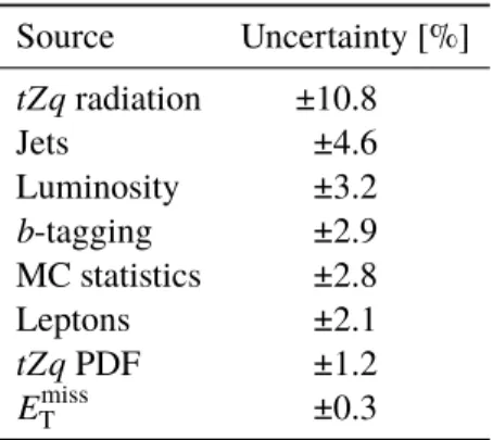
The effects of the above uncertainties on the number of signal events are summarised in Table 4. This does not include the impact of the background uncertainties.
Background The uncertainties on the normalisation of the various background processes use either the uncertainty estimated in Section 6, or the uncertainties on the cross-section predictions (tt V + ttH).
The latter uncertainty is 13 % [20]. For the tt sample, the systematic effects due to uncertainties on the scale and radiation are studied. After all selection criteria have been applied, the effect is too small to distinguish a systematic variation from statistical fluctuations; therefore it is not used.
9 Results
Using the 141 selected events, a maximum-likelihood fit is performed to extract the tZq signal strength, µ , defined as the ratio of the measured signal yield to the NLO Standard Model expectation. The statistical analysis of the data employs a binned likelihood function L ( µ, ~ θ), constructed as the product of Poisson probability terms, to estimate µ [51]. The likelihood is maximised on the NN output distribution in the signal region.
The impact of systematic uncertainties on the signal and background expectations is described by nuisance
parameters, θ ~ , which are each parametrised by a Gaussian or log-normal constraint for each bin of the
NN output distribution. If the variation of the uncertainty in each bin is consistent with being due to
Table 4: Breakdown of the impact of the systematic uncertainties on the t Z q signal in order of decreasing effect.
Details of the systematics are provided in the text.
Source Uncertainty [%]
tZq radiation ±10.8
Jets ±4.6
Luminosity ±3.2
b -tagging ±2.9
MC statistics ±2.8
Leptons ±2.1
tZq PDF ±1.2
E
missT
±0.3
statistical fluctuations, only the overall change in normalisation is included as a nuisance parameter. The uncertainties are set to be symmetric in the fit, using the average of the variations up and down. The expected numbers of signal and background events in each bin are functions of ~ θ . The test statistic, q
µ, is constructed according to the profile likelihood ratio: q
µ= − 2 ln[ L ( µ, θ ~ ˆˆ )/L ( µ, ˆ ~ θ)], where ˆ ˆ µ and ~ θ ˆ are the parameters that maximise the likelihood, and ~ θ ˆˆ are the nuisance parameter values that maximise the likelihood for a given µ . This test statistic is used to measure the compatibility of the background-only hypothesis with the observed data.
Figure 4 shows the NN discriminant in the signal region with background normalisations, signal normal- isation, and nuisance parameters adjusted by the profile likelihood fit.
The results for the numbers of fitted signal and background events are summarised in Table 5. The total uncertainty on the number of fitted events includes the effect of correlations, which are large among the background sources, as the O
NNdistributions have a similar shape. The strongest correlation is found to be between the diboson and the Z + jets contributions and it is about −0.5 for both the Asimov dataset and the data. The table also shows the result of a fit to the Asimov dataset [51].
Table 5: Fitted yields in the signal region for the Asimov dataset and the data. The fitted numbers of events contain the statistical plus systematic uncertainties.
Channel Number of events
Asimov dataset Real data
tZq 35 ± 9 26 ± 8
tt + tW 18 ± 7 17 ± 7
Z + jets 37 ± 11 34 ± 11
Diboson 53 ± 13 48 ± 12
tt V + ttH + tWZ 20 ± 3 19 ± 3
Total 163 ± 12 143 ± 11
After performing the binned maximum-likelihood fit and estimating the total uncertainty, the fitted value
for µ is 0 . 75 ± 0 . 21 (stat.) ± 0 . 17 (syst.) ± 0 . 07 (th.). The error on µ includes the tZq NLO cross-section
uncertainty given in Section 3. This is not taken into account when evaluating the cross-section. The
ONN
Entries / 0.1
10 20 30 40
50 ATLAS Preliminary = 13 TeV, 36.1 fb
-1s
Data tZq +tW Z+jets tt Diboson
H+tWZ t V+t Uncertainty tt
O
NN0 0.1 0.2 0.3 0.4 0.5 0.6 0.7 0.8 0.9 1
Data / Pred.
0 1 2
Figure 4: Post-fit neural-network output distributions in the signal region. Signal and backgrounds are normalised to the expected number of events after the fit. The uncertainty band includes both statistical and systematic uncertainties as obtained by the fit.
statistical uncertainty on the cross-section is determined by performing a fit to the data, only includ- ing the statistical uncertainties. The total systematic uncertainty is determined by subtracting this value in quadrature from the total uncertainty. The cross-section for tZq production is measured to be 600 ± 170 (stat.) ± 140 (syst.) fb, assuming a top-quark mass of m
t= 172.5 GeV.
The probability p
0
of obtaining a result at least as signal-like as observed in the data if no signal were present is calculated using the test statistic q
µ=0= − 2 ln[ L( µ = 0 , θ ~ ˆˆ )/L ( µ, ˆ ~ θ) ˆ ] in the asymptotic approximation [51]. The observed p
0value is 1.3 × 10
−5. The resulting significance is 4 . 2 σ , to be compared with the expected significance of 5 . 4 σ .
10 Conclusion
The cross-section for tZq production has been measured using 36.1 fb
−1of data collected by the ATLAS experiment at the LHC in 2015 and 2016 at a centre-of-mass energy of
√ s = 13 TeV. Evidence for the
signal is obtained with a measured (expected) significance of 4 . 2 σ (5 . 4 σ ). The measured cross-section
is 600 ± 170 (stat.) ± 140 (syst.) fb. This result is in agreement with the predicted SM tZq cross-section
calculated at NLO to be 800 fb, which has an uncertainty due to variation of the factorisation and
renormalisation scales of
+6−7..14%.
References
[1] CDF Collaboration, F. Abe et al., Observation of top quark production in pp ¯ collisions, Phys. Rev. Lett. 74 (1995) 2626, arXiv: hep-ex/9503002 [hep-ex] .
[2] D0 Collaboration, S. Abachi et al., Observation of the top quark, Phys. Rev. Lett. 74 (1995) 2632, arXiv: hep-ex/9503003 [hep-ex] .
[3] D0 Collaboration, V. M. Abazov et al., Observation of Single Top Quark Production, Phys. Rev. Lett. 103 (2009) 092001, arXiv: 0903.0850 [hep-ex] .
[4] CDF Collaboration, T. Aaltonen et al.,
First Observation of Electroweak Single Top Quark Production, Phys. Rev. Lett. 103 (2009) 092002, arXiv: 0903.0885 [hep-ex] . [5] CDF and D0 Collaborations, T. A. Aaltonen et al.,
Observation of s-channel production of single top quarks at the Tevatron, Phys. Rev. Lett. 112 (2014) 231803, arXiv: 1402.5126 [hep-ex] .
[6] ATLAS Collaboration, Measurement of the production cross-section of a single top quark in association with a W boson at 8 TeV with the ATLAS experiment, JHEP 01 (2016) 064, arXiv: 1510.03752 [hep-ex] .
[7] CMS Collaboration, Observation of the associated production of a single top quark and a W boson in pp collisions at √
s = 8 TeV, Phys. Rev. Lett. 112 (2014) 231802, arXiv: 1401.2942 [hep-ex] .
[8] C. Patrignani et al., Review of Particle Physics, Chin. Phys. C40 (2016) 100001.
[9] J. Campbell, R. K. Ellis and R. Röntsch,
Single top production in association with a Z boson at the LHC, Phys. Rev. D 87 (2013) 114006, arXiv: 1302.3856 [hep-ph] .
[10] J. Chang, K. Cheung, J. S. Lee and C.-T. Lu,
Probing the Top-Yukawa Coupling in Associated Higgs production with a Single Top Quark, JHEP 05 (2014) 062, arXiv: 1403.2053 [hep-ph] .
[11] CMS Collaboration, Search for associated production of a Z boson with a single top quark and for t Z flavour-changing interactions in pp collisions at √
s = 8 TeV, (2017), arXiv: 1702.01404 [hep-ex] .
[12] ATLAS Collaboration, Measurement of the t tW ¯ and t t Z ¯ production cross sections in pp collisions at √
s = 8 TeV with the ATLAS detector, JHEP 11 (2015) 172, arXiv: 1509.05276 [hep-ex] . [13] ATLAS Collaboration, Measurement of the t¯ t Z and t tW ¯ production cross sections in multilepton
final states using 3 . 2 fb
−1of pp collisions at √
s = 13 TeV with the ATLAS detector, Eur. Phys. J. C 77 (2017) 40, arXiv: 1609.01599 [hep-ex] .
[14] CMS Collaboration, Observation of top quark pairs produced in association with a vector boson in pp collisions at √
s = 8 TeV, JHEP 01 (2016) 096, arXiv: 1510.01131 [hep-ex] . [15] ATLAS Collaboration, The ATLAS Experiment at the CERN Large Hadron Collider,
JINST 3 (2008) S08003.
[16] ATLAS Collaboration, Trigger Menu in 2016, ATL-DAQ-PUB-2017-001, 2017,
url: https://cds.cern.ch/record/2242069 .
[17] Performance of the ATLAS Trigger System in 2015, Eur. Phys. J. C 77 (2017) 317, arXiv: 1611.09661 [hep-ex] .
[18] S. Agostinelli et al., GEANT4: A Simulation toolkit, Nucl. Instrum. Meth. A 506 (2003) 250.
[19] ATLAS Collaboration, The ATLAS Simulation Infrastructure, Eur. Phys. J. C 70 (2010) 823, arXiv: 1005.4568 [hep-ex] .
[20] J. Alwall et al., The automated computation of tree-level and next-to-leading order differential cross sections, and their matching to parton shower simulations, JHEP 07 (2014) 079,
arXiv: 1405.0301 [hep-ph] . [21] J. Pumplin et al.,
New generation of parton distributions with uncertainties from global QCD analysis, JHEP 07 (2002) 012, arXiv: hep-ph/0201195 [hep-ph] .
[22] R. Frederix, E. Re and P. Torrielli,
Single-top t-channel hadroproduction in the four-flavour scheme with POWHEG and aMC@NLO, JHEP 09 (2012) 130, arXiv: 1207.5391 [hep-ph] .
[23] T. Sjöstrand, S. Mrenna and P. Z. Skands, PYTHIA 6.4 Physics and Manual, JHEP 05 (2006) 026, arXiv: hep-ph/0603175 .
[24] P. Z. Skands, Tuning Monte Carlo Generators: The Perugia Tunes, Phys. Rev. D82 (2010) 074018, arXiv: 1005.3457 [hep-ph] .
[25] R. D. Ball et al., Parton distributions for the LHC run II, JHEP 04 (2015) 40, arXiv: 1410.8849 [hep-ph] .
[26] P. Nason, A New method for combining NLO QCD with shower Monte Carlo algorithms, JHEP 11 (2004) 040, arXiv: hep-ph/0409146 .
[27] S. Frixione, P. Nason and C. Oleari,
Matching NLO QCD computations with Parton Shower simulations: the POWHEG method, JHEP 11 (2007) 070, arXiv: 0709.2092 [hep-ph] .
[28] S. Alioli, P. Nason, C. Oleari and E. Re, A general framework for implementing NLO calculations in shower Monte Carlo programs: the POWHEG BOX, JHEP 06 (2010) 043,
arXiv: 1002.2581 [hep-ph] .
[29] T. Sjöstrand, S. Mrenna and P. Z. Skands, A Brief Introduction to PYTHIA 8.1, Comput. Phys. Commun. 178 (2008) 852, arXiv: 0710.3820 [hep-ph] .
[30] ATLAS Collaboration, ATLAS Pythia 8 tunes to 7 TeV data, ATL-PHYS-PUB-2014-021, 2014, url: https://cds.cern.ch/record/1966419 .
[31] ATLAS Collaboration, Electron reconstruction and identification efficiency measurements with the ATLAS detector using the 2011 LHC proton–proton collision data,
Eur. Phys. J. C 74 (2014) 2941, arXiv: 1404.2240 [hep-ex] . [32] ATLAS Collaboration,
Electron identification measurements in ATLAS using √
s = 13 TeV data with 50 ns bunch spacing, ATL-PHYS-PUB-2015-041, 2015, url: https://cds.cern.ch/record/2048202 .
[33] ATLAS Collaboration, Electron and photon energy calibration with the ATLAS detector using data collected in 2015 at √
s = 13 TeV, ATL-PHYS-PUB-2016-015, 2016,
url: https://cds.cern.ch/record/2203514 .
[34] ATLAS Collaboration, Electron efficiency measurements with the ATLAS detector using the 2015 LHC proton–proton collision data, ATLAS-CONF-2016-024, 2016,
url: https://cds.cern.ch/record/2157687 .
[35] ATLAS Collaboration, Muon reconstruction performance of the ATLAS detector in proton–proton collision data at √
s = 13 TeV, Eur. Phys. J. C 76 (2016) 292, arXiv: 1603.05598 [hep-ex] . [36] M. Cacciari and G. P. Salam, Dispelling the N
3myth for the k
tjet-finder,
Phys. Lett. B 641 (2006) 57, arXiv: hep-ph/0512210 .
[37] M. Cacciari, G. P. Salam and G. Soyez, The anti- k
tjet clustering algorithm, JHEP 04 (2008) 063, arXiv: 0802.1189 .
[38] ATLAS Collaboration, Jet energy measurement and its systematic uncertainty in proton–proton collisions at √
s = 7 TeV with the ATLAS detector, Eur. Phys. J. C 75 (2015) 17, arXiv: 1406.0076 [hep-ex] .
[39] ATLAS Collaboration, Performance of b -Jet Identification in the ATLAS Experiment, JINST 11 (2016) P04008, arXiv: 1512.01094 [hep-ex] .
[40] ATLAS Collaboration, Performance of missing transverse momentum reconstruction in proton–proton collisions at √
s = 7 TeV with ATLAS, Eur. Phys. J. C 72 (2012) 1844, arXiv: 1108.5602 [hep-ex] .
[41] M. Feindt, A Neural Bayesian Estimator for Conditional Probability Densities, 2004, arXiv: 0402093v1 .
[42] M. Feindt and U. Kerzel, The NeuroBayes Neural Network Package, Nucl. Instrum. Meth. A559 (2006) 190.
[43] ATLAS Collaboration,
Electron and photon energy calibration with the ATLAS detector using LHC Run 1 data, Eur. Phys. J. C 74 (2014) 3071, arXiv: 1407.5063 [hep-ex] .
[44] ATLAS Collaboration, Jet Calibration and Systematic Uncertainties for Jets Reconstructed in the ATLAS Detector at √
s = 13 TeV, ATL-PHYS-PUB-2015-015, 2015, url: https://cds.cern.ch/record/2037613 .
[45] ATLAS Collaboration, Jet energy resolution in proton–proton collisions at √
s = 7 TeV recorded in 2010 with the ATLAS detector, Eur. Phys. J. C 73 (2013) 2306, arXiv: 1210.6210 [hep-ex] . [46] ATLAS Collaboration, Performance of missing transverse momentum reconstruction with the
ATLAS detector in the first proton–proton collisions at √
s = 13 TeV, ATL-PHYS-PUB-2015-027, 2015, url: https://cds.cern.ch/record/2037904 .
[47] ATLAS Collaboration, Calibration of b -tagging using dileptonic top pair events in a
combinatorial likelihood approach with the ATLAS experiment, ATLAS-CONF-2014-004, 2014, url: https://cds.cern.ch/record/1664335 .
[48] ATLAS Collaboration,
Calibration of the performance of b -tagging for c and light-flavour jets in the 2012 ATLAS data, ATLAS-CONF-2014-046, 2014, url: https://cds.cern.ch/record/1741020 .
[49] J. Butterworth et al., PDF4LHC recommendations for LHC Run II, J. Phys. G 43 (2016) 023001,
arXiv: 1510.03865 [hep-ph] .
[50] ATLAS Collaboration,
Luminosity determination in pp collisions at √
s = 8 TeV using the ATLAS detector at the LHC, Eur. Phys. J. C 76 (2016) 653, arXiv: 1608.03953 [hep-ex] .
[51] G. Cowan, K. Cranmer, E. Gross and O. Vitells,
Asymptotic formulae for likelihood-based tests of new physics,
Eur. Phys. J. C 71 (2011) 1554, [Erratum: Eur. Phys. J. C 73 (2013) 2501],
arXiv: 1007.1727 [physics.data-an] .
Appendix
µ µ /
∆
− 0.1 0 0.1
resolution soft term
miss
E T
Muon identification -tagging scale factor b
JES flavour composition normalisation t
t
Luminosity Jet energy resolution tZq theory Diboson normalisation tZq radiation
θ
∆
0 )/
θ θ - (
− 2 0 2
ATLAS Preliminary
= 13 TeV, 36.1 fb
-1s
signal
µ Pre-fit impact on
signal