ATLAS-CONF-2020-024 30July2020
ATLAS CONF Note
ATLAS-CONF-2020-024
28th July 2020
Measurement of the production cross section of isolated photon pairs in pp collisions at 13 TeV with
the ATLAS detector
The ATLAS Collaboration
A measurement of prompt photon-pair production in proton-proton collisions at
√
𝑠
=13 TeV is presented. The data were recorded by the ATLAS detector at the LHC with an integrated luminosity of 139 fb
−1. Events with two photons in the well-instrumented region of the detector are selected, and the photons are required to be isolated and have 𝐸
T, 𝛾1(2)
> 40
(30
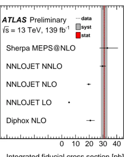
)GeV for the leading (sub-leading) photon. The differential cross section as functions of several observables for the diphoton system are measured in the fiducial volume and compared to theoretical predictions from state-of-the-art Monte Carlo and fixed-order calculations. The measured integrated cross section is compatible with the predictions from next-to-next-to-leading order and multileg-merged calculations. Predictions from lower-orders in perturbative QCD fail to agree with data within their estimated theoretical uncertainties. Agreement between measured differential cross sections and the most accurate predictions is generally good where expected, showing a clear necessity to take higher-order perturbative QCD corrections into account.
© 2020 CERN for the benefit of the ATLAS Collaboration.
Reproduction of this article or parts of it is allowed as specified in the CC-BY-4.0 license.
1 Introduction
The production of a prompt-photon pair in proton-proton collisions is one of the cornerstone processes of the LHC physics program. Most prominently, it is vital for searching for and studying the properties of resonances decaying into photon pairs, such as the Higgs boson or other neutral particles. The main background to resonant diphoton production originates from the continuum production of such pairs, which is the subject of this note. Despite the electromagnetic nature of this process, diphoton production in hadron colliders involves strong-interaction dynamics; theoretical predictions are therefore highly non-trivial and measurements are necessary to scrutinise and validate such predictions.
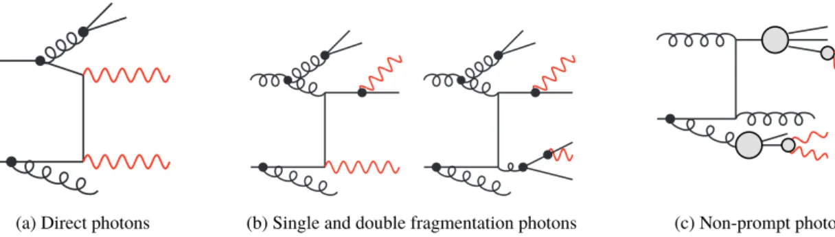
Prompt photons are those not produced in hadron decays. Non-resonant photons can be produced by various mechanisms in 𝑝 𝑝 collisions at the LHC. In a theoretical or Monte Carlo (MC) picture, prompt photons are typically subdivided into two different production mechanisms: the “direct” production mode, represented by a 𝑞 𝑞 ¯
→𝛾 𝛾 𝑡 -channel diagram at leading order; and the “fragmentation” component with a hard 𝛾 +jet or dijet configuration and subleading photon emissions in a resummed approach. A schematic representation exemplifies these photon production mechanisms in Fig. 1(a) and Fig. 1(b), respectively. By far the most abundant source of photons in 𝑝 𝑝 collisions are hadron decays like 𝜋
0 →𝛾 𝛾 , cf. Fig. 1(c).
These are explicitly not the focus of this note and are in fact considered as background. To suppress the contribution of photons from hadron decays (non-prompt), photons are required to be isolated from hadronic activity in their vicinity.
In this analysis the diphoton production at the LHC in 𝑝 𝑝 collisions at
√
𝑠
=13 TeV is measured with the full Run-2 dataset. Previous diphoton cross section measurements have been performed at 7 TeV by CMS [1, 2] and ATLAS [3, 4], and at 8 TeV by ATLAS [5]. Other prompt-photon measurements have studied single photon production in CMS [6] and in ATLAS [7–11] at
√
𝑠
=13 TeV.
The main challenge and source of uncertainty on the experimental side is the estimation of the background from non-prompt photons in jet events. In this analysis, a sophisticated background decomposition fit is used to estimate the background contributions using a data-driven technique. The background-subtracted yield is then corrected for detector effects using an iterative unfolding procedure. Differential cross section measurements are presented in a fiducial region as functions of several kinematic observables of the photon pair. State-of-the-art theoretical predictions from fixed-order calculations and from MC event generators are compared to the data.
(a) Direct photons (b) Single and double fragmentation photons (c) Non-prompt photons
Figure 1: Schematic of theoretical photon pair production mechanisms. The black dots represent resummed Bremsstrahlung e.g. from a fragmentation function or parton shower, while the grey circles represent hadronisation and hadron decay processes.
2 ATLAS detector
The ATLAS experiment [12] at the LHC is a multi-purpose particle detector with a forward-backward symmetric cylindrical geometry and a near 4 𝜋 coverage in solid angle.
1It consists of an inner tracking detector surrounded by a thin superconducting solenoid providing a 2 T axial magnetic field, electromagnetic and hadron calorimeters, and a muon spectrometer.
The inner tracking detector covers the pseudorapidity range
|𝜂
|< 2 . 5. It consists of silicon pixel, silicon microstrip, and transition radiation tracking detectors.
The calorimeter system covers the pseudorapidity range
|𝜂
|< 4 . 9. Within the region
|𝜂
|< 3 . 2, electromagnetic (EM) calorimetry is provided by barrel and endcap high-granularity lead/liquid-argon (LAr) calorimeters, with an additional thin LAr presampler covering
|𝜂
|< 1 . 8, to correct for energy loss in material upstream of the calorimeters. Hadronic calorimetry is provided by the steel/scintillating-tile calorimeter, segmented into three barrel structures within
|𝜂
|< 1 . 7, and two copper/LAr hadronic endcap calorimeters. The solid angle coverage is completed with forward copper/LAr and tungsten/LAr calorimeter modules optimised for electromagnetic and hadronic measurements respectively.
The muon spectrometer surrounds the calorimeters and is based on three large air-core toroidal supercon- ducting magnets with eight coils each. The field integral of the toroids ranges between 2.0 and 6.0 T m across most of the detector. The muon spectrometer includes a system of precision tracking chambers and fast detectors for triggering.
A two-level trigger system is used to select events. The first-level trigger is implemented in hardware and uses a subset of the detector information to reduce the accepted rate to at most nearly 100 kHz. This is followed by a software-based trigger that reduces the accepted event rate to 1 kHz on average depending on the data-taking conditions [13].
3 Data and simulated samples
3.1 Data samples
The data used in this measurement were recorded by the ATLAS detector in 𝑝 𝑝 collisions at
√
𝑠
=13 TeV during the LHC Run-2 data taking period. Events were selected using a diphoton trigger requiring the presence in the EM calorimeter of two clusters of energy depositions with transverse energy above 35 GeV and 25 GeV for the leading and subleading clusters, respectively. Only events taken during stable beam conditions and satisfying detector and data-quality requirements [14] are considered. These requirements ensure that the calorimeters and inner tracking detectors are in nominal operation.
The total integrated luminosity of the collected sample after trigger and data quality requirements amounts to 139 fb
−1. Multiple 𝑝 𝑝 interactions (pile-up) can occur in the same bunch crossing, with 34 simultaneous interactions produced on average. The efficiency of the diphoton triggers with respect to the offline selection
1ATLAS uses a right-handed coordinate system with its origin at the nominal interaction point (IP) in the centre of the detector and the𝑧-axis along the beam pipe. The𝑥-axis points from the IP to the centre of the LHC ring, and the𝑦-axis points upwards. Cylindrical coordinates (𝑟 , 𝜙) are used in the transverse plane, 𝜙being the azimuthal angle around the𝑧-axis.
The pseudorapidity is defined in terms of the polar angle𝜃as𝜂=−ln tan(𝜃/2). Angular distance is measured in units of Δ𝑅≡p
(Δ𝜂)2+ (Δ𝜙)2.
presented in the next section ranges between 96% and 100% [15] as a function of the transverse energy ( 𝐸
T
) of the sub-leading photon.
3.2 Simulated event samples for signal and background processes
Samples of events from a MC simulation are used for the subtraction of subdominant background as well as for cross checks of the subtraction of the dominant background, for the unfolding of detector effects, and as theoretical predictions in the final comparison to the measured data.
All simulated event samples include pile-up effects, as well as the effect on the detector response due to interactions from bunch crossings before or after the one containing the hard interaction. Pile-up interactions deteriorate the resolution of the calorimetric variables. The MC samples are reweighted to match the pile-up noise in data events. All samples were processed through the ATLAS detector simulation based on Geant4 [16] using the same reconstruction algorithms as used in data.
Diphoton signal samples.
Simulated samples of prompt diphoton production were generated with two different programs, Sherpa [17] and Pythia8 [18]. The nominal samples used in the analysis are simulated with the Sherpa v2.2 generator [17]. Their size amounts to approximately twice the equivalent luminosity of data. In this setup, matrix elements for 𝑝 𝑝
→𝛾 𝛾
+0 , 1 𝑗
2at next-to-leading order (NLO) accuracy in the strong coupling constant 𝛼
𝑠and 𝑝 𝑝
→𝛾 𝛾
+2 , 3 𝑗 at leading-order (LO) accuracy are matched and merged with the Sherpa parton shower based on Catani-Seymour dipoles [19, 20] using the MEPS@NLO prescription [21, 22]. The virtual QCD correction for matrix elements at NLO accuracy is provided by the OpenLoops library [23, 24]. Samples were generated using the NNPDF3.0 next-to-next-to-leading order (NNLO) set [25] of parton distribution functions (PDF), along with the dedicated set of tuned parton-shower parameters developed by the Sherpa authors. Both the direct and fragmentation component of isolated photon production are included by setting the merging scale dynamically in the scheme of Ref. [26], and a photon isolation requirement based on a smooth cone [27] is used with 𝑛
=2, 𝛿
=0 . 1 and 𝜀
=0 . 1. In addition, the loop-induced 𝑔𝑔
→𝛾 𝛾 box process is included in these samples at LO accuracy.
An alternative signal sample was generated with Pythia8. Direct production was simulated using LO matrix elements for 𝑝 𝑝
→𝛾 𝛾 and showered in Pythia8 v8.186 [18] using the NNPDF2.3 LO [28] PDF set with the A14 shower tune [29]. The same framework was used to generate the single-fragmentation component based on LO matrix elements for 𝑝 𝑝
→𝛾 𝑗 with one additional photon produced in the parton shower, and the double-fragmentation component based on LO matrix elements for 𝑝 𝑝
→𝑗 𝑗 with both additional photons produced in the parton shower. No photon isolation requirement is applied in these samples at the generator level.
Electron background sources.
Since electrons can fake photons or even radiate real photons, background processes with prompt electron production from Drell-Yan processes, 𝑍
/𝛾
∗(→𝑒 𝑒
)and 𝑊
(→𝑒 𝜈
), are considered and estimated from MC simulation. The samples used to estimate these backgrounds were generated using Powheg-Box v2 [30, 31] interfaced to the Pythia8 v8.186 [18] parton shower model with the AZNLO set of tuned parameters [32]. Photos++ 3.52 [33] was used for QED emissions from electroweak vertices and charged leptons. The W/Z samples are normalised to NNLO cross sections calculated with FEWZ [34]. Even though the impact is negligible, a poor modelling of the 𝑝
T(
𝑍
)spectrum
2Here and in the following,𝑗refers to “jet”, which at matrix-element level corresponds to a quark or gluon.
in the 𝑍
(→𝑒 𝑒
)sample is corrected for using data/MC correction factors from the measurement in Ref. [35].
𝜸 𝒋 background.
While this background is determined in a data-driven approach, Sherpa v2.2 [17]
simulations of the 𝑝 𝑝
→𝛾
+1 , 2 𝑗 @NLO
+3 , 4 𝑗 @LO process are used for cross checks. The setup is otherwise equivalent to the diphoton signal samples described above.
4 Data selection and observables definition
The photon and event selections are explained in Sections 4.1 and 4.2, respectively, and the definition of the observables is included in Section 4.3.
4.1 Photon reconstruction and selection
Photon candidates are reconstructed from a cluster of energy depositions in the electromagnetic calorimeter [36, 37]. The photon energy is calibrated as described in Ref. [38], and its uncertainty depends on the 𝐸
Tand 𝜂 of the photon, with a value of 0 . 2%
−0 . 4% for central photons with transverse energy in the intermediate range dominating this analysis. Photons which undergo conversion in the inner detector are distinguished from unconverted photons by associating inner detector tracks to the photon and have generally a lower energy scale uncertainty.
The momenta of the photon candidates are corrected for the position of their associated reconstructed primary interaction vertex. The associated vertex is chosen among all reconstructed vertices, which are required to have at least two inner detector tracks assigned with transverse momentum ( 𝑝
T
) > 0 . 5 GeV.
The measured trajectories of the two photons, along with the reconstructed vertex information in the event, are used as inputs to a neural-network algorithm trained on simulation to select the most probable primary vertex [39, 40] for the photon candidates.
The identification of photons is based on multiple variables that quantify the longitudinal and lateral shape of the electromagnetic shower produced by the photon. Requirements on these shower-variables are used to identify photons. A detailed description of all variables and selections for the ‘tight’ photon identification used in this analysis is given in Ref. [41]. The identification variables 𝑓
side
(energy fraction outside of core cells) and 𝑤
𝑠3
(lateral shower width) are used to define control regions. These variables use information in the finely segmented first layer of the electromagnetic calorimeter and are sensitive to differences between candidates from prompt photons and background candidates e.g. from the two collimated photons of a neutral hadron decay. If the photon candidate fails the requirement on at least one of these two variables but passes all other selections of the ‘tight’ photon identification, it enters into one of the control regions enriched in candidates from non-prompt photons.
The isolation measurement is based on calorimeter information [41]. The initial isolation variable is defined
as the sum of the transverse energy computed from topological clusters of calorimeter cells [42] in a cone
of
Δ𝑅
=0 . 2 around the photon candidate direction. The transverse energy deposited in the rectangular
window around the photon candidate and the expected transverse energy leaking out of this core region
into the isolation cone are subtracted from the initial transverse isolation energy. Furthermore, effects of
pile-up and from the underlying event (UE) are corrected for on an event-by-event based estimation using
the ambient transverse energy density [43]. This density is determined as the median energy density of jets in the two regions of
|𝜂
|< 1 . 5 and 1 . 5 <
|𝜂
|< 3 using the 𝑘
𝑡-algorithm [44] with radius 𝑅
=0 . 5. The resulting isolation variable 𝐸
iso,0.2T
can be negative and photons with negative isolation values are kept. The background contribution decreases with the 𝐸
T
of the photon, and therefore, an 𝐸
T
dependent isolation requirement is better suited than a constant one. The requirement 𝐸
iso,0.2T, 𝛾1(2)
< 0 . 05
·𝐸
T, 𝛾1(2)
is used in the signal region. It is relaxed to 0 . 05
·𝐸
T, 𝛾1(2)
< 𝐸
iso,0.2T, 𝛾1(2)
< 0 . 15
·𝐸
T, 𝛾1(2)
for photon candidates in the control regions.
4.2 Event selection
The event selection is based on the properties of the leading ( 𝛾
1
) and subleading ( 𝛾
2
) photon candidates in each event. Requirements are applied on the transverse energy, the pseudorapidity, the isolation and the identification of the two photons as well as on their angular separation. The signal region is defined by the criteria summarised in Table 1. With these signal requirements approximately 4 709 000 events are selected in the data.
Table 1: Overview of the signal selection at the detector level and at the particle level.
Selection Detector level Particle level
Photon kinematics 𝐸
T, 𝛾1(2)
> 40
(30
)GeV,
|𝜂
𝛾|< 2 . 37 excluding 1 . 37 <
|𝜂
𝛾|< 1 . 52 Photon identification tight stable, not from hadron decay
Photon isolation 𝐸
iso,0.2T, 𝛾
< 0 . 05
·𝐸
T, 𝛾
𝐸
iso,0.2T, 𝛾
< 0 . 09
·𝐸
T, 𝛾
Diphoton topology 𝑁
𝛾 ≥2,
Δ𝑅
𝛾 𝛾> 0 . 4
4.2.1 Details of the particle-level selection
The particle level selection, to which the data are unfolded to (cf. Sec. 6) closely follows the detector-level signal requirements, and is also shown in Table 1. Some aspects are clarified in detail in the remainder of this section.
The particle-level event selection in MC samples takes the leading two photons into account and vetoes the event if one of them is not prompt or fails the fiducial cuts.
The transverse isolation energy at particle level is determined as the sum of the transverse energies of all stable particles
3excluding particles from pile-up, muons, neutrinos and the photon itself. Furthermore, to match the side effects of the UE subtraction at detector level also at the particle-level
4, a final-state based subtraction using the same method as described in Sec. 4.1 is applied. The value of the isolation requirement at the particle level (0.09) is chosen to be different from the one at the detector level (0.05).
This difference accounts for the non-compensating nature of the ATLAS calorimeter, and the particle-level value has been optimised to minimise the number of events where photons pass a detector-level isolation requirement but fail the particle-level one, or vice versa.
3Stable particles are defined as those with a decay length𝑐𝜏 >10 mm.
4While there is no pile-up at particle level, there are still other effects, e.g. multiple parton interactions, that can cause such a subtraction procedure to have an influence.
4.3 Observables
Cross sections are measured differentially as functions of several observables defined for the diphoton system:
• Transverse energy 𝐸
T, 𝛾 1
( 𝐸
T, 𝛾
2
) of the leading (subleading) photon,
• Invariant mass 𝑚
𝛾 𝛾and transverse momentum 𝑝
T, 𝛾 𝛾
of the photon pair,
• Acoplanarity 𝜋
− Δ𝜙
𝛾 𝛾=
𝜋
−𝜙
𝛾1−
𝜙
𝛾2
of the photons,
• Transverse component of 𝑝
T, 𝛾 𝛾
with respect to the thrust axis:
𝑎
T, 𝛾 𝛾 =2
·𝑝
𝑥 , 𝛾1
𝑝
𝑦 , 𝛾2−
𝑝
𝑦 , 𝛾1
𝑝
𝑥 , 𝛾2
𝑝
®T, 𝛾 1− ®
𝑝
T, 𝛾 2
,
where 𝑝
𝑥(𝑦), 𝛾1(2)
are the 𝑥
(𝑦
)-component of the leading (subleading) photon momenta, while
®
𝑝
T, 𝛾1− ®
𝑝
T, 𝛾
2
is the transverse component of the momentum difference of both photons.
• The angular variable defined as:
𝜙
∗𝜂 =
tan
𝜋
− Δ𝜙
𝛾 𝛾
2 sin 𝜃
∗𝜂 =
tan
𝜋
− Δ𝜙
𝛾 𝛾
2
s
1
−
tanh
Δ
𝜂
𝛾 𝛾2
2
,
where
Δ𝜙
𝛾 𝛾
is the azimuthal distance between the two photons mapped into the range
[0 , 𝜋
], and
Δ𝜂
𝛾 𝛾 =𝜂
𝛾1−
𝜂
𝛾2
. Angular variables are typically measured with better resolution than the photon energy. Therefore, a particular reference frame that allows 𝜙
∗𝜂
to be expressed in terms of angular variables only, denoted by the subscript 𝜂 and described in Ref. [45], is used in order to optimise the resolution. In particular, 𝜙
∗𝜂
is ideal to probe QCD effects because it probes similar dynamics as 𝑝
T, 𝛾 𝛾, but with a significantly better resolution in the low- 𝑝
T, 𝛾 𝛾
region. A similar argument holds for 𝑎
T, 𝛾 𝛾
.
• The scattering angle with respect to the beam axis in the Collins-Soper frame [46]:
|
cos 𝜃
∗|(CS)=sinh
(Δ𝜂
𝛾 𝛾) q1
+ (𝑝
T, 𝛾 𝛾/
𝑚
𝛾 𝛾)2·
2 𝐸
T, 𝛾 1
𝐸
T, 𝛾 2
𝑚
2 𝛾 𝛾
=
𝑝
+𝛾1
𝑝
−𝛾2 −
𝑝
−𝛾1
𝑝
+𝛾2
𝑚
𝛾 𝛾 ·q𝑚
2𝛾 𝛾+
𝑝
2 T, 𝛾 𝛾
,
with 𝑝
±𝛾 =
𝐸
𝛾±𝑝
𝑧 , 𝛾, where 𝐸
𝛾is the energy of the photon and 𝑝
𝑧 , 𝛾is the 𝑧 -component of the momentum of the photon.
5 Background estimation
Reconstructed photon pairs can appear in the detector from a variety of sources beyond prompt production
processes. These are summarised in this section along with details about how they are estimated and
subtracted from the selected events to give the actual 𝛾𝛾 signal yield. As a result, the purity of the diphoton
signalis
(60 . 4
+−32..08)%, where the uncertainties account for systematic and statistical sources as described in
Sec. 7.
The
jet backgroundarises from jets mis-identified as photons and constitutes the main background. It consists of 𝛾 𝑗 (
(19 . 9
±1 . 2
)%), 𝑗𝛾 (
(10 . 1
+−10..09)%), or 𝑗𝑗 (
(6 . 3
+−11..20)%) events with one or two jets mis-identified as photons, respectively. The data-driven determination is described in detail in Sec. 5.1. The notation 𝑗𝛾 ( 𝑦 𝑗 ) here and in the following refers to the component where the leading (sub-leading) photon candidate stems from a mis-identified jet, while in 𝑗𝑗 events both photon candidates do.
Another
(2 . 6
±0 . 1
)% of the sample corresponds to the
electron background (ee), with the electrons
5being mis-identified as or radiating photons. The main process contributing to this background is Drell-Yan production. It is estimated using the MC simulation described in Sec. 3.2 and is only visible in analysis regions with 𝑚
𝛾 𝛾 ∼𝑚
Z
.
Finally,
(0 . 6
+−00..53)% of the sample is associated to
pile-up background (PU), i.e. pairs of𝛾 𝑗 events from different 𝑝 𝑝 collisions on the same bunch crossing. It is determined with a data-driven approach discussed in Sec. 5.2.
The selected diphoton data sample can also contain signal events in which the two photon candidates come from the decay of a Higgs boson. Their contribution to the signal region is predicted to be 0 . 2%
of the integrated signal and increases to a few percent in the relevant 𝑚
𝛾 𝛾bin. This contribution is not subtracted from the data as background, since it is a genuine part of prompt-photon pair production and thus considered to be signal.
5.1 Jet background
The background from jets mis-identified as prompt photons is estimated using a data-driven method, extrapolating the amount from multiple control regions enriched in background to the signal region. This is done performing a likelihood fit and is an extension to the two-photon case of the “two-dimensional sideband” technique used in the single photon analyses [7, 8, 10, 47–53]. It is similar to the method used in previous diphoton analyses [3, 4]. The fit is performed separately in each bin of each observable; in the description presented below, the labels that refer to the bins in each observable are not included.
To define the control regions, the selection on two almost independent jet-photon discriminant variables are reversed with respect to the signal selection: the photon 𝑓
side
and 𝑤
𝑠3
shower-shape variables and the photon isolation, as defined in Sec. 4.1.
In addition to the signal region, where both photons pass both isolation and identification criteria, 15 background control regions are defined representing all possible combinations where at least one photon fails at least one of the criteria. These regions are labelled by index 𝑖
=1 . . . 16, with 𝑖
=1 being the signal region. As an example, the isolation distributions for the sub-leading photon in MC signal events and those events in data that fail the identification criteria, and can be considered as background, are shown in Fig. 2.
To decompose the event sample, probability functions 𝑓
𝑝 ,𝑖corresponding to the probability of an event from process 𝑝
∈ {𝛾𝛾 , 𝛾 𝑗 , 𝑗𝛾 , 𝑗𝑗 , 𝑒𝑒, PU
}to fall in diphoton category 𝑖 are defined. They are constructed as a product of the four probabilities for the each of the two photon candidates to fulfil both the isolation
5Electron here and in the following always refers to an electron or a positron.
−0.1 −0.05 0 0.05 0.1 0.15 0.2 0.25 0.3
γ2
/ ET, γ2
T,
Eiso
0 0.01 0.02 0.03 0.04 0.05 0.06 0.07 0.08
Arbitrary units
region Signal
control region Background
MC signal (Sherpa)
Background control-region data
ATLAS Preliminary = 13 TeV, 139 fb-1
s
Figure 2: Relative photon isolation distribution for the subleading photon candidate as extracted from the Sherpa diphoton sample (black histogram) and from mis-identified jets extracted from data events in the non-tight control region (blue histogram).
and identification requirements of the category according to 𝑓
𝑝 ,𝑖 =𝑓
𝑝 ,𝑖(𝜀
iso𝑝 ,1
, 𝜀
iso𝑝 ,2
, 𝑅
iso𝑝
, 𝜀
id𝑝 ,1
, 𝜀
id𝑝 ,2
, 𝑅
id𝑝
, 𝑅
iso−id𝑝 ,1
, 𝑅
iso−id𝑝 ,2 )
=
𝜀
iso𝑝 ,1
𝜀
iso𝑝 ,2
𝜀
id𝑝 ,1
𝜀
id𝑝 ,2
for 𝑖
=1
𝜀
iso𝑝 ,1 (
1
−𝜀
iso𝑝 ,2)
𝜀
id𝑝 ,1
𝜀
id𝑝 ,2
for 𝑖
=2
(
1
−𝜀
iso𝑝 ,1)
𝜀
iso𝑝 ,2
𝑅
iso𝑝
𝜀
id𝑝 ,1
𝜀
id𝑝 ,2
for 𝑖
=3
(
1
−𝜀
iso𝑝 ,1) (
1
−𝜀
iso𝑝 ,2
𝑅
iso𝑝 )
𝜀
id𝑝 ,1
𝜀
id𝑝 ,2
for 𝑖
=4
𝜀
iso 𝑝 ,1𝜀
iso 𝑝 ,2𝑅
iso−id 𝑝 ,2𝜀
id𝑝 ,1 (
1
−𝜀
id𝑝 ,2)
for 𝑖
=5
𝜀
iso𝑝 ,1 (
1
−𝜀
iso𝑝 ,2
𝑅
iso−id𝑝 ,2 )
𝜀
id𝑝 ,1 (
1
−𝜀
id𝑝 ,2)
for 𝑖
=6
(
1
−𝜀
iso𝑝 ,1)
𝜀
iso𝑝 ,2
𝑅
iso 𝑝𝑅
iso−id𝑝 ,2
𝜀
id𝑝 ,1 (
1
−𝜀
id𝑝 ,2)
for 𝑖
=7
(
1
−𝜀
iso𝑝 ,1) (
1
−𝜀
iso𝑝 ,2
𝑅
iso 𝑝𝑅
iso−id𝑝 ,2 )
𝜀
id𝑝 ,1 (
1
−𝜀
id𝑝 ,2)
for 𝑖
=8
𝜀
iso 𝑝 ,1𝑅
iso−id 𝑝 ,1𝜀
iso𝑝 ,2 (
1
−𝜀
id𝑝 ,1)
𝜀
id 𝑝 ,2𝑅
id𝑝
for 𝑖
=9
𝜀
iso 𝑝 ,1𝑅
iso−id𝑝 ,1 (
1
−𝜀
iso𝑝 ,2) (
1
−𝜀
id𝑝 ,1)
𝜀
id 𝑝 ,2𝑅
id𝑝
for 𝑖
=10
(
1
−𝜀
iso 𝑝 ,1𝑅
iso−id 𝑝 ,1 )𝜀
iso𝑝 ,2
𝑅
iso𝑝 (
1
−𝜀
id𝑝 ,1)
𝜀
id 𝑝 ,2𝑅
id𝑝
for 𝑖
=11
(
1
−𝜀
iso𝑝 ,1
𝑅
iso−id𝑝 ,1 ) (
1
−𝜀
iso𝑝 ,2
𝑅
iso𝑝 ) (
1
−𝜀
id𝑝 ,1)
𝜀
id𝑝 ,2
𝑅
id𝑝
for 𝑖
=12
𝜀
iso 𝑝 ,1𝑅
iso−id𝑝 ,1
𝜀
iso𝑝 ,2
𝑅
iso−id𝑝 ,2 (
1
−𝜀
id𝑝 ,1) (
1
−𝜀
id 𝑝 ,2𝑅
id𝑝)
for 𝑖
=13
𝜀
iso 𝑝 ,1𝑅
iso−id𝑝 ,1 (
1
−𝜀
iso𝑝 ,2
𝑅
iso−id𝑝 ,2 ) (
1
−𝜀
id𝑝 ,1) (
1
−𝜀
id 𝑝 ,2𝑅
id𝑝)
for 𝑖
=14
(
1
−𝜀
iso𝑝 ,1
𝑅
iso−id𝑝 ,1 )
𝜀
iso𝑝 ,2
𝑅
iso𝑝
𝑅
iso−id𝑝 ,2 (
1
−𝜀
id𝑝 ,1) (
1
−𝜀
id𝑝 ,2
𝑅
id𝑝)
for 𝑖
=15
(
1
−𝜀
iso 𝑝 ,1𝑅
iso−id𝑝 ,1 ) (
1
−𝜀
iso 𝑝 ,2𝑅
iso 𝑝𝑅
iso−id𝑝 ,2 ) (
1
−𝜀
id𝑝 ,1) (
1
−𝜀
id 𝑝 ,2𝑅
id𝑝)
for 𝑖
=16 .
(1)
Here, 𝜀
iso 𝑝 , 𝑛( 𝜀
id𝑝 , 𝑛
) is the efficiency of the leading ( 𝑛
=1) or subleading ( 𝑛
=2) photon candidate, to fulfill the signal region isolation (identification) requirement with respect to the looser requirements that include the control regions. The correlation correction factors 𝑅 account either for correlations between the isolation and identification of one photon candidate, 𝑅
iso−id𝑝 , 𝑛
, or for correlations between the isolation (identification) of both candidates, 𝑅
iso𝑝
( 𝑅
id𝑝
). 𝑅
=1 corresponds to no correlation between the relevant variables, while values below or above unity indicate a certain degree of positive or negative correlation, respectively.
The expected number of events 𝑛
exp𝑖
in each region 𝑖 can then be written as:
𝑛
exp𝑖 =
𝑛
𝛾𝛾𝜀
id 𝛾𝛾 ,1𝜀
iso𝛾𝛾 ,1
𝜀
id 𝛾𝛾 ,2𝜀
iso𝛾𝛾 ,2
𝑓
𝛾𝛾 ,𝑖+𝑁
𝛾 𝑗𝑓
𝛾 𝑗 ,𝑖 +𝑁
𝑗𝛾𝑓
𝑗𝛾 ,𝑖+𝑁
𝑗𝑗𝑓
𝑗𝑗 ,𝑖 +𝑁
𝑒𝑒𝑓
𝑒𝑒,𝑖 +𝑁
PU
𝑓
PU,𝑖
. (2) Here, 𝑁
𝛾𝛾, 𝑁
𝛾 𝑗, 𝑁
𝑗𝛾, and 𝑁
𝑗𝑗are the total number of events attributed to the signal or background processes, respectively. The parameter of interest, i.e. the number of 𝛾𝛾 events in the signal region, is given by 𝑛
𝛾𝛾≡𝑁
𝛾𝛾·𝜀
id𝛾𝛾 ,1
𝜀
iso 𝛾𝛾 ,1𝜀
id𝛾𝛾 ,2
𝜀
iso𝛾𝛾 ,2
. The total number of electron background events, 𝑁
𝑒𝑒, and of pile-up background events, 𝑁
PU
, are fixed parameters in the fit. The other parameters are either pre-determined as described in Sec. 5.1.1 (thus reducing the number of parameters from Eq. (1) to Eq. (2)), or left as floating nuisance parameters in the likelihood fit. The likelihood function for a given observable bin is given by
L (
𝑛
𝛾𝛾, 𝜃
| ®𝑛
obs) =Ö𝑖
𝑛
exp𝑖 (
𝑛
𝛾𝛾, 𝜃
)𝑛obs𝑖𝑛
obs𝑖
!
𝑒
−𝑛exp 𝑖 (𝑛𝛾𝛾, 𝜃)
, (3)
where 𝜃 is the set of 13 nuisance parameters floating in the fit in addition to 𝑛
𝛾𝛾: 𝜃
={𝑁
𝛾 𝑗, 𝜀
id𝛾 𝑗 ,2
, 𝜀
iso𝛾 𝑗 ,2
, 𝑁
𝑗𝛾, 𝜀
id𝑗𝛾 ,1
, 𝜀
iso𝑗𝛾 ,1
, 𝑁
𝑗𝑗, 𝜀
id𝑗𝑗 ,1
, 𝜀
iso𝑗𝑗 ,1
, 𝜀
id𝑗𝑗 ,2
, 𝜀
iso𝑗𝑗 ,2
, 𝑅
id𝑗𝑗
, 𝑅
iso𝑗𝑗 }
. (4)
All nuisance parameters are associated with jets misidentified as photons, for which the reconstruction efficiencies and correlations are not known accurately, thus motivating this sophisticated approach.
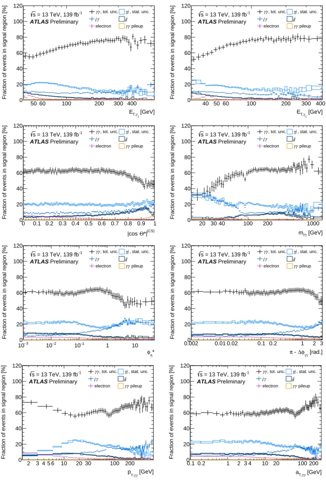
The result of the fit for the inclusive data sample can be seen for each of the 16 regions in Fig. 3.
As mentioned above, results are also obtained in each observable bin separately, and the equivalent decomposition in the signal region is displayed differentially in Fig. 4. The purity of the 𝛾𝛾 signal process ranges from 35% at low invariant mass up to 80% at high 𝐸
T
.
5.1.1 Fit model input parametersThe fit model introduced in the previous section relies on several pre-determined parameters, which are described below. In order to take into account the systematic uncertainties on these input parameters, the fit is repeated with systematic variations of the corresponding parameter values.
Signal parameters: 𝜺𝜸𝜸,id
1,𝜺𝜸𝜸,id
2,𝑹𝜸𝜸id,𝜺iso𝜸𝜸,
1,𝜺𝜸𝜸,iso
2,𝑹𝜸𝜸iso,𝑹𝜸𝜸,iso−id
1 and 𝑹𝜸𝜸,iso−id
2
The values of the eight 𝛾𝛾 signal parameters are extracted from the MC simulation based on the
Sherpa signal sample, corrected to match the isolation and identification variable distributions
in data [41, 54]. These parameters are extracted as a function of each observable for which
the differential cross section is measured. Uncertainties on these parameters due to the detector
simulation and theory modelling, in particular for the isolation distribution, are taken into account as
described in Sec. 7.2 and 7.3.
PP 1
PF 2
FP 3
FF 4
PP 5
PF 6
FP 7
FF 8
PP 9
PF 10
FP 11
FF 12
PP 13
PF 14
FP 15
FF
0
16500 1000 1500 2000 2500 3000 3500 4000 4500
10
3×
Events
Region index and isolation status Pass-Pass id. Pass-Fail id. Fail-Pass id. Fail-Fail id.
Diphoton identification region Data
signal γ γ γj γ j jj electron
pileup γ γ
= 13 TeV, 139 fb
-1s
ATLAS Preliminary
Figure 3: Event yields of the inclusive data sample in the 16 diphoton regions. Both the observed counts and the post-fit predictions of the signal and each background component are shown. Labels “PP/PF/FP/FF” are used to denote the isolation status (“P”=pass, “F”=fail) of the leading and subleading photon candidates.
Correlation between isolation and identification: 𝑹𝜸𝒋,iso−id
2 and 𝑹iso𝒋𝜸,−id
1
The correlation between isolation and identification for jets mis-identified as photons is parametrised by the 𝑅
iso−id𝑗 ≡
𝑅
iso−id𝛾 𝑗 ,2 =
𝑅
iso−id𝑗𝛾 ,1
correction factor. A twofold approach is used to estimate it. First, a 𝛾 𝑗 MC sample is used to estimate this parameter from simulation, yielding 𝑅
iso−id,MC
𝑗 =
0 . 99
±0 . 03
(stat) without a significant trend as a function of 𝐸
T
within the limited MC statistics. In addition to the MC study, a 𝛾 𝑗 -rich validation region in data is constructed by requiring the subleading photon to fail an isolation requirement based on the sum of the transverse momenta of charged-particle tracks coming from the primary vertex, and subtracting the contamination of 𝛾𝛾 events in that region using the signal MC simulation. With a higher statistical power in data, an increase in correlation as a function of 𝐸
T
is observed. This dependency is extrapolated to the signal region using the MC simulation. For the final results, an average of the MC and data results is used differentially, with central values varying in a range of 0 . 93 < 𝑅
iso−id𝑗
< 1 with 𝐸
T
, and with uncertainties propagated, as described in Sec. 7.1.
Correlation between isolation in𝜸 𝒋and 𝒋𝜸events: 𝑹𝜸𝒋isoand𝑹iso𝒋𝜸
The correction factor 𝑅
iso𝑝
parametrises the correlation between the isolation variables of the two photon candidates. For the signal pdf, this parameter is extracted from MC as 𝑅
iso𝛾𝛾
. A similar extraction for fake photons from 𝛾 𝑗 MC samples alone is not possible because of the limited statistical precision available. A slight correlation is expected, as found for the signal pdf, where 0 . 95 < 𝑅
iso𝛾𝛾
< 1.
It can also be extracted in 𝑗𝑗 background events, where 𝑅
iso𝑗𝑗
is left to float in the fit and yields values in the range 0 . 9 < 𝑅
iso𝑗𝑗
< 1. For the 𝛾 𝑗 and 𝑗𝛾 backgrounds, 𝑅
iso 𝛾 𝑗 =𝑅
iso𝑗𝛾 =
0 . 95
±0 . 05 is chosen in
50 60 100 200 300 400 [GeV]
γ1
ET,
0 20 40 60 80 100 120
Fraction of events in signal region [%]
, tot. unc.
γ
γ γj, stat. unc.
γ
j jj
electron γγ pileup
= 13 TeV, 139 fb-1
s
ATLAS Preliminary
40 50 60 100 200 300 400
[GeV]
γ2
ET,
0 20 40 60 80 100 120
Fraction of events in signal region [%]
, tot. unc.
γ
γ γj, stat. unc.
γ
j jj
electron γγ pileup
= 13 TeV, 139 fb-1
s
ATLAS Preliminary
0 0.1 0.2 0.3 0.4 0.5 0.6 0.7 0.8 0.9 1
*|(CS)
Θ
|cos 0
20 40 60 80 100 120
Fraction of events in signal region [%]
, tot. unc.
γ
γ γj, stat. unc.
γ
j jj
electron γγ pileup
= 13 TeV, 139 fb-1
s
ATLAS Preliminary
20 30 40 100 200 1000
[GeV]
γ
mγ
0 20 40 60 80 100 120
Fraction of events in signal region [%]
, tot. unc.
γ
γ γj, stat. unc.
γ
j jj
electron γγ pileup
= 13 TeV, 139 fb-1
s
ATLAS Preliminary
−3
10 10−2 10−1 1 10
η* φ 0
20 40 60 80 100 120
Fraction of events in signal region [%]
, tot. unc.
γ
γ γj, stat. unc.
γ
j jj
electron γγ pileup
= 13 TeV, 139 fb-1
s
ATLAS Preliminary
0.002 0.01 0.02 0.1 0.2 1 2 3
[rad.]
γ
φγ
∆ π - 0
20 40 60 80 100 120
Fraction of events in signal region [%]
, tot. unc.
γ
γ γj, stat. unc.
γ
j jj
electron γγ pileup
= 13 TeV, 139 fb-1
s
ATLAS Preliminary
2 3 4 5 6 10 20 30 100 200
[GeV]
γ γ
pT,
0 20 40 60 80 100 120
Fraction of events in signal region [%]
, tot. unc.
γ
γ γj, stat. unc.
γ
j jj
electron γγ pileup
= 13 TeV, 139 fb-1
s
ATLAS Preliminary
0.1 0.2 1 2 3 4 10 20 100 200
[GeV]
γ γ
aT,
0 20 40 60 80 100 120
Fraction of events in signal region [%]
, tot. unc.
γ
γ γj, stat. unc.
γ
j jj
electron γγ pileup
= 13 TeV, 139 fb-1
s
ATLAS Preliminary
Figure 4: Sample decomposition as a function of each observable. For the𝛾𝛾signal fraction, the total uncertainty is shown, while for the background fractions only the data and Monte Carlo statistical uncertainty component is shown.
all regions of phase space, thus the uncertainties cover the extreme cases.
Photon isolation and identification efficiencies in𝜸 𝒋: 𝜺𝜸𝒋,1iso ,𝜺iso𝒋𝜸,2,𝜺id𝜸𝒋,1,𝜺id𝒋𝜸,2
For the 𝛾 𝑗 and 𝑗𝛾 background components, isolation and identification efficiencies for the prompt photons are derived from the 𝛾𝛾 signal MC sample. The underlying assumption is cross-checked by comparing these efficiencies to the ones derived in the 𝛾 𝑗 Sherpa MC sample. The efficiencies are compatible within statistical uncertainties.
Identification correlation in𝜸 𝒋events: 𝑹𝜸𝒋idand 𝑹id𝒋𝜸
The correlation between the identification of the two objects is in general very low. This is cross- checked with MC simulation for the 𝛾𝛾 signal process. Performing the fit with extreme values of 𝑅
id𝛾 𝑗
and 𝑅
id𝑗𝛾
determined from MC simulation results in negligible variations of the final result. The assumption 𝑅
id𝛾 𝑗 =
𝑅
id𝑗𝛾 =
1 is thus kept without an additional uncertainty.
5.2 Pile-up of multiple single-photon events
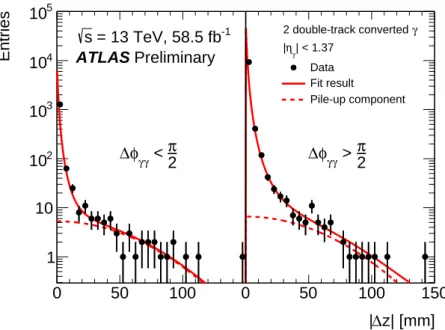
Pairs of 𝛾 𝑗 events from different 𝑝 𝑝 collisions in the same bunch crossing can form a diphoton final state in the detector. The normalisation of this background is estimated using a fit to the data. The shape of the background in the diphoton observables is based on MC simulations. Details of the procedure are given below.
The background is estimated selecting diphoton candidate events in data in which both photons converted to electron-positron pairs within the detector material and both are required to have
|𝜂
|< 1 . 45
6. The resulting tracks are required to be reconstructed in the inner tracking detector and the conversion point is required to be measured within the volume of the silicon pixel or strip detector. These tracks thus provide precise information about the longitudinal position 𝑧
𝛾of the vertex along the beam in which the photon is produced, thus providing means to differentiate whether the two photons come from the same primary vertex. This information is used in a two-component template fit to
Δ𝑧
=|𝑧
𝛾1−
𝑧
𝛾2|
, as can be seen in Fig. 5.
The first component of the template, representing the distribution of pile-up events in
Δ𝑧 , is considered to be a convolution of the two individual longitudinal Gaussian 𝑧
PV
distributions which have a width of 𝜎
𝑧 =35 mm, resulting in a Gaussian with a width of 𝜎
Δ𝑧 =√
2
×𝜎
𝑧. The second component of the template, representing the non-pile-up contribution, is taken as a power-law function. To extract the fraction of the pile-up events, the power-law parameters and the normalisation of each component are fitted simultaneously to the measured
Δ𝑧 distribution. The fit is performed in two regions simultaneously,
Δ𝜙
𝛾𝛾< 𝜋
/2 and
Δ𝜙
𝛾𝛾> 𝜋
/2, where the pile-up background fraction in the first region is about a factor 10 higher than in the second. The fit yields an uncertainty of 𝛿
PUfit =±
15% on the pile-up background fraction.
The event yield resulting from this fit still contains contributions from fake photons, which are subtracted in the main background fit also for pile-up events. To avoid a double subtraction, the nominal background fit is performed for the events with
Δ𝑧 > 48 mm to determine the fraction of prompt 𝛾𝛾 events within the pile-up contribution. The large uncertainty of 𝛿
PUsignal=±
50% on this fraction is of statistical nature due to the low number of input events, and is added in quadrature with the 𝛿
PUfit
to form the total uncertainty on the pile-up background propagated to the final results, as described in Sec. 7.
6The fraction of converted photons is fairly constant as a function of photon𝐸
Tand𝜂and well modelled in MC. The conversion events can thus be used directly for an extrapolation to the full dataset.
0 50 100 0 50 100 150 z| [mm]
∆
| 1
10 102
103
104
105
Entries
2 < π
γ
φγ
∆ ∆φγγ > 2π
= 13 TeV, 58.5 fb-1
s
ATLAS Preliminary
Data Fit result
Pile-up component γ 2 double-track converted
| < 1.37 ηγ
|
Figure 5: The two-component template fit to determine the global normalisation of pile-up events is shown. Data events in which each of the two photon candidates is associated with two inner detector tracks are used for the fit.
The dashed lines represent the pile-up-like component of the total template marked with a solid line.
With the normalisation of the pile-up background fixed, the shape of this background in the fiducial phase space and as a function of each observable is derived using a sample of pseudo-events. Events in this sample are constructed by overlaying two separate reconstructed events from a 𝛾 𝑗 MC simulation. This shape is combined with the normalisation determined as above and fed into the background estimation fit as a pre-determined component.
6 Correction to particle level
Detector effects due to finite resolution and inefficient detection of particles have to be corrected for in order to be able to compare results from different experiments and to allow comparisons to theory without detector simulation. The unfolding procedure is applied to the background subtracted distribution at the detector level in three steps.
First the measured distribution is corrected for the fraction of reconstructed MC events that do not pass the particle-level selection. The contribution of these unmatched reconstructed events is estimated using the signal MC samples. The main source of unmatched photons are due to the transverse energy and the photon isolation requirements. The particle-level selection is chosen close to the detector-level selection to reduce the influence of this correction.
The second step is to correct for detector resolution effects which cause migrations from one particle-level
bin to multiple detector-level bins. For this step, an iterative unfolding method [55] based on Bayes’ theorem
is used. Response matrices parametrise these migrations and are constructed from simulated events passing
both the detector-level and particle-level selections. A first iteration of the migration correction uses the
particle-level prediction as the prior input. The prior then gets updated with each of the three iterations
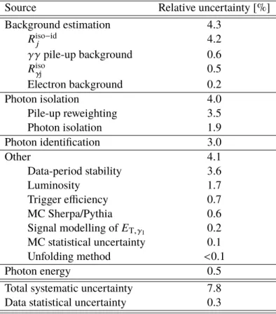
Table 2: Breakdown of the relative uncertainties on the integrated fiducial cross section measurement.
Source Relative uncertainty [%]
Background estimation 4.3
𝑅
iso−id𝑗
4.2
𝛾 𝛾 pile-up background 0.6
𝑅
iso𝛾j
0.5
Electron background 0.2
Photon isolation 4.0
Pile-up reweighting 3.5
Photon isolation 1.9
Photon identification 3.0
Other 4.1
Data-period stability 3.6
Luminosity 1.7
Trigger efficiency 0.7
MC Sherpa/Pythia 0.6
Signal modelling of 𝐸
T, 𝛾
1