Measurement of the production cross-section of

(1)

ATLAS-CONF-2019-047 17October2019

ATLAS CONF Note

ATLAS-CONF-2019-047

1st October 2019

Measurement of the production cross-section of J / ψ and ψ ( 2S ) mesons at high transverse momentum in p p collisions at √

s = 13 TeV with the ATLAS detector

The ATLAS Collaboration

The measurements of the prompt and non-prompt differential cross-sections of

J/ψ

and

ψ(

2S

)

mesons with

p_T

between 60 and 360 GeV and rapidity range

|y| <

2 are reported. Furthermore, the measurements of the non-prompt fractions of

ψ(

2

S)

and

J/ψ

, and prompt and non-prompt production ratios of

ψ(

2

S)

to

J/ψ

are presented. The analysis is performed using

pp

collision data recorded by the ATLAS detector at

√s =

13 TeV collected between 2015 and 2018, corresponding to 139 fb

⁻¹

of integrated luminosity.

Reproduction of this article or parts of it is allowed as specified in the CC-BY-4.0 license.

(2)

1 Introduction

Studies involving heavy quarkonia provide a unique insight into the nature of Quantum Chromodynamics (QCD) near the boundary of perturbative and non-perturbative regimes. However, despite the long history, the investigation of quarkonium production in hadronic collisions still presents significant challenges to both theory and experiment.

In high energy hadronic collisions, charmonium states can be produced either from the short-lived QCD sources (referred to as ‘prompt’ production), or from long-lived sources such as decays of beauty hadrons (referred to as ‘non-prompt’ production). These can be separated experimentally by measuring the distance between the production and decay vertices of the quarkonium state. Effects of feeddown from higher charmonium states contributes to production of

J/ψ

mesons, whereas no significant contribution occurs for the

ψ(

2S

)

meson. While the FONLL calculations [1, 2] within the framework of perturbative QCD have been reasonably successful in describing the non-prompt contributions, a satisfactory understanding of the prompt production mechanisms is still to be achieved.

The methods developed within non-relativistic QCD (NRQCD) approach provide a framework for describing these processes, giving rise to a variety of models with variable success and different predictive power. In particular, Ref. [3] introduced a number of phenomenological parameters — long-distance matrix elements (LDMEs) — which can be extracted from the fits to the experimental data, and are hence expected to describe the cross-sections and differential spectra reasonably well [4–7]. But several attempts to build a universal ‘library’ of LDMEs to be used to describe a wider range of measurements such as polarisation of quarkonia [8–11], their associated production [12, 13] or the production of quarkonium in a wider range of processes, such as photo- and electro-production, have not been particularly successful [14–18]. A combination of ATLAS results with the cross-section and polarisation measurements from CMS [7, 19, 20], LHCb [6] and ALICE [21] now includes a variety of charmonium production characteristics in a wide kinematic range, thus providing a wealth of information for a new generation of theoretical models.

It is hence increasingly important to broaden the scope of comparison between theory and experiment by providing a broader variety of experimental information on quarkonium production in a wider kinematic range. ATLAS has previously measured the inclusive differential cross-section of the

J/ψ

production at

√s =

7 and 8 TeV [4], as well as the differential cross sections of the production of

χ_c

states [22], and

ψ(

2S

)

production in its

J/ψππ

decay mode [5]. In most of these measurements ATLAS exploited a dimuon trigger with the muon

p_T

threshold of 4 GeV, with the high-

p_T

reach limited mainly by the trigger performance to about 100 GeV. This note describes a measurement of the

J/ψ

(

ψ(

2S

)

) meson production, in their dimuon decay mode, at

√s =

13 TeV in the range of high transverse momenta (

p_T

) from 60 to 360 GeV (60–140 GeV), well beyond the existing measurements. This was made possible by the use of a high-

p_T

single-muon trigger, which ran unprescaled throughout Run II of the LHC, and the high integrated luminosity of 139 fb

⁻¹

accumulated by the ATLAS detector in the period between 2015 and 2018. The measurements include the double-differential cross section of the two vector charmonium states (separately for prompt and non-prompt production mechanisms), the non-prompt fraction for each state, and the production ratios of

ψ(

2S

)

over

J/ψ

.

The note is organised as follows: a brief description of the ATLAS detector and event selection are given in Section 2. The analysis strategy is explained in Section 3, followed by the systematic studies in Section 4.

The results are presented in Section 5, followed by the summary in Section 6.

(3)

2 The ATLAS detector

The ATLAS detector [23] is a general-purpose particle physics detector with a forward-backward symmetric cylindrical geometry and near 4

π

coverage in solid angle. The inner tracking sub-detector (ID) consists of a silicon pixel detector, a silicon microstrip detector, and a transition radiation tracker. The ID is surrounded by a thin superconducting solenoid providing a 2 T magnetic field and by high-granularity liquid-argon sampling electromagnetic calorimeters. An iron-scintillator tile calorimeter provides hadronic coverage in the central rapidity range. The endcap and forward regions are instrumented with liquid-argon calorimeters for both electromagnetic and hadronic measurements. The muon spectrometer (MS) surrounds the calorimeters and consists of a system of precision tracking chambers and detectors for triggering, inside a toroidal magnetic field.

Data for this analysis were taken during LHC proton-proton collision runs at

√s

= 13 TeV in years 2015 to 2018, with total integrated luminosity of 139 fb

⁻¹

.

3 Analysis strategy

3.1 Event selection

The selected events are required to contain a pair of oppositely charged muons of high quality (using the Tight identification requirements defined in Ref. [24]), selected by a single muon trigger with

p_T

threshold of 50 GeV. The analysis requires each muon to have

p_T >

4 GeV and

|η| <

2

.

4,

¹

with at least one of the muons having

p_T >

52

.

5 GeV and matched to the trigger object. The two ID tracks are fitted to a common vertex, selected to have a dimuon mass within the range 2

.

6

< m_µµ <

4

.

2 GeV. The transverse distance

L_xy

between the primary vertex and the dimuon vertex is used to calculate the pseudo-proper decay time

τ= m p_T

L_xy

c

(1)

where

m_µµ

and

p_T

are the reconstructed mass and transverse momentum of the dimuon system, respectively, and

c

is the speed of light. The primary vertex is chosen as the reconstructed collision interaction vertex closest in the

z

coordinate to the intersection of the dimuon’s trajectory with the beam axis in the

z

–

r

plane.

In the case of more than one selected candidate in an event, all candidates are retained.

3.2 Cross section determination

The phase space of this measurement is divided into 12 intervals in dimuon

p_T

covering the range from 60 to 360 GeV, and 3 intervals in absolute rapidity

|y|

with boundaries at 0, 0.75, 1.5 and 2.0, thus producing 36 ‘analysis bins’ overall. In each

(p_T,|y|)

analysis bin, dimuon candidates are assigned a weight to correct for inefficiencies from trigger and reconstruction effects, and a 2-dimensional unbinned maximum likelihood fit is applied to the distribution of the weighted dilepton candidates. The 2 dimensions are the

1ATLAS uses a right-handed coordinate system with its origin at the nominal interaction point (IP) in the centre of the detector and thez-axis along the beam pipe. Thex-axis points from the IP to the centre of the LHC ring, and they-axis points upward.

Cylindrical coordinates(r, φ)are used in the transverse plane,φbeing the azimuthal angle around thez-axis. The pseudorapidity is defined in terms of the polar angleθasη=−ln tan(θ/2).

(4)

dilepton mass

m

and the pseudo-proper decay time

τ

. Each candidate is weighted with the product of reconstruction efficiency weight

w_reco

, the trigger efficiency weight

w_trig

, and a decay length correction weight

w_dec

calculated as

w_reco =

1

_reco(µ⁺)_reco(µ⁻),

w_trig =

1

− (

1

−_trig(µ⁺))(

1

−_trig(µ⁻)),

(2)

w_dec =

1

_dec,

where single-muon reconstruction and trigger efficiencies

_reco

and

_trig

are extracted from data-driven efficiency maps obtained by the tag-and-probe method [24] using various dimuon resonances, while

_dec

takes into account the loss of efficiency in cases where a non-prompt dimuons are produced in the decay of a very long-lived parent which decays beyond one or more layers of the ID. Once weights for each candidate are determined, the data across the four years are combined and unbinned maximum likelihood fits performed to each analysis bin, described in detail in Section 3.4. The fits produce corrected yields

N_ψ^P^,^NP

for prompt (P) and non-prompt (NP)

ψ

states, where

ψ = J/ψ, ψ(

2

S)

. The main parameters determined from the fit are the corrected yields,

N_ψ^P^,^NP

, where

ψ = J/ψ, ψ(

2

S)

, for prompt (P) and non-prompt (NP)

J/ψ

and

ψ(

2S

)

mesons, and their respective non-prompt fractions and production ratios.

The respective double-differential cross sections are then calculated using the full covariance matrix as:

d²σ^P^,^NP(pp→ψ)

dp_Tdy × B(ψ →µ⁺µ⁻)=

1

A(ψ) C_BMC_AP

N_ψ^P^,^NP

∆p_T ∆y ∫

Ldt,

(3)

where

∆p_T

and

∆y

are bin widths in dimuon transverse momentum and rapidity respectively, while

∫ Ldt

is the integrated luminosity.

A(ψ)

is the kinematic acceptance, defined as the probability that a

ψ

candidate with a (true) transverse momentum and rapidity in a given analysis bin passes the acceptance requirement on muon parameters:

p_T(µ₁) >

52

.

5 GeV,

p_T(µ₂) >

4 GeV,

|η(µ₁, µ₂)| <

2

.

4, for a given

ψ

mass. Since the acceptance calculation is performed using truth-level kinematic variables, while the yield determination is done in intervals of reconstructed

p_T

, a bin migration correction

C_BM

is applied at a later stage of the analysis. Another factor,

C_AP

, derived from simulated decays of

ψ

to dimuons, is applied to correct for the dependence of the efficiencies on pileup conditions, and for biases in the efficiencies because of angular correlations between the two muons.

The non-prompt fractions for

ψ= J/ψ, ψ(

2S

)

are calculated as

F_ψ^NP(p_T,y)= N_ψ^NP

N_ψ^P+N_ψ^NP.

(4)

Finally, production ratios of

ψ(

2S

)

over

J/ψ

are calculated, separately for prompt and non-prompt production mechanisms, as

R^P^,^NP(p_T,y)=

A(ψ(

2S

)) A(J/ψ)

−1 N_ψ(^P^,^NP

2S)

N_J/ψ^P^,^NP.

(5)

3.3 Acceptance

The kinematic acceptance

A(ψ)

in each analysis bin, defined as the probability for a

ψ

meson with a given

p_T

and

|y|

to fall into the fiducial volume of the detector (defined by the muon selection criteria described above), is calculated using a generator-level ‘accept-reject’ simulation. Nominal values, assuming an isotropic distribution, of the correction factors, 1

/A(ψ)

, averaged over the analysis bins decrease from about 4.1 in the lowest

p_T

bin to 1.02 in the highest, with no sizeable dependence on rapidity.

Since the spin-alignment of the

ψ

states may affect acceptance, a number of extreme cases that lead to the largest variations of acceptance within the phase space of this measurement are identified and used to calculate the range in which the results may vary under any physically allowed spin-alignment assumption, and derived also from ‘accept-reject’ simulations. The spin-alignment correction factors, relative to the nominal values, for longitudinal (transverse) polarisation vary from 0.62 (1.18) at the lowest

p_T

to 1.02 (0.99) at the highest

p_T

for

J/ψ

(

ψ(

2S

)

) mesons, again with no sizeable rapidity dependence, and are presented in the Appendix as sets of additional correction factors.

3.4 Fit model

The fit model PDF is described by a sum of seven terms, corresponding to the prompt and non-prompt components for the two charmonium states and background processes:

PDF

(m, τ)=Õ⁷

i=1

κ_iP_i(m, τ)

(6)

For

i=

2–7 each term is factorised into a function

f_i

of dimuon mass

m

and a function

h_i

of pseudo-proper decay time

τ

, where the latter is convolved with the decay time resolution function

R(τ)

:

P_i(m, τ)= f_i(m) · (h_i(τ) ⊗R(τ))

(7)

The term with

i=

1 has a similar structure, but allows for some correlations between

m

and

τ

(see below).

R(τ)

is parameterised as a weighted sum of three Gaussians, with

σ₂=

2

σ₁

and

σ₃ =

3

σ₁

. The relative weights of these Gaussians are free parameters, as is

σ₁

. The central values of all three Gaussians are fixed at zero.

Table 1 summarises the form of each of the 7 components and is explained in detail below.

The terms corresponding to

i=

1

,

2 describe the prompt and non-prompt

J/ψ

signal respectively; similarly, terms 3

,

4 correspond to prompt and non-prompt signal from

ψ(

2S

)

. The mass lineshape of the

J/ψ

(

ψ(

2S

)

) peak is parametrised as a weighted sum of a Gaussian

G₁(G₂)

and a Crystal Ball function

C B₁(C B₂)

. These parameterisations are the same for prompt and non-prompt components. The decay time dependence of the prompt components (

i=

1 and

i=

3) is given by a delta-function (before smearing),

δ(τ)

, while for the non-prompt components (

i=

2 and

i=

4) the decay time dependencies are exponential, with independent slopes.

In the term with

i=

1, the product of the Gaussian term in

f₁(m)

and the leading Gaussian term in

R(τ)

is replaced by a bivariate Gaussian in

m

and

τ

to take into account an empirically observed correlation

between the measured values of these quantities.

(6)

The term with

i=

5 describes the prompt background with decay time dependence given by a delta-function (before smearing),

δ(τ)

, and mass dependence parameterised by a superposition of the first three Bernstein polynomials

B₀_,₁(t)=

1

−t, B₁_,₁(t)=t, B₀_,₂(t)=(

1

−t)²,

(8) where

t=(m(

GeV

) −

2

.

6

)/

1

.

6 is designed to vary between 0 and 1.

Terms 6 and 7 correspond to non-prompt backgrounds, with decay time dependences given by a single-sided and a symmetric double-sided exponentials respectively, with free independent slopes. Both terms have exponential dependence on mass, with independent slope parameters.

i Type P/NP f_i(m) h_i(τ)

1 J/ψ P ωG₁(m)+(1−ω)C B₁(m) δ(τ) 2 J/ψ NP ωG₁(m)+(1−ω)C B₁(m) E₁(τ) 3 ψ(2S) P ωG₂(m)+(1−ω)C B₂(m) δ(τ) 4 ψ(2S) NP ωG₂(m)+(1−ω)C B₂(m) E₂(τ)

5 Bkg P B δ(τ)

6 Bkg NP E₄(m) E₅(τ)

7 Bkg NP E₆(m) E₇(|τ|)

Notation Function

G Gaussian

C B Crystal Ball

E Exponential

B Bernstein polynomials

Table 1: Parameterisation of the fit model. Notation is explained in the text and in the table on the right. Correlation betweenmandτis introduced in one of the sub-terms fori=1, see the text for details.

A fit is performed in each analysis bin using an unbinned maximum likelihood method, in the range of dimuon masses from 2.6 to 4.2 GeV and the decay time range between

−

1 and 11 ps. Out of 30 parameters 19 are determined from the fit, with the rest fixed to the values pre-determined from various test fits.

Uncertainties due to variations of the fit models and assumptions on the fixed parameters are tested at the stage of systematic studies, described in Section 4. In particular, it was found that a reliable determination of the cross section of prompt and non-prompt production for the

ψ(

2S

)

meson is only possible up to

p_T =

140 GeV. For

p_T >

140 GeV the yield of

ψ(

2S

)

was fixed to a constant fraction of the yield of

J/ψ

, using information from the fits at lower transverse momentum.

Figure 1 shows the mass and pseudo proper decay time projections of the fits in several randomly chosen analysis bins, together with associated pull distributions.

The main parameters determined from the fit are the yields of

J/ψ

and

ψ(

2S

)

states and their respective non-prompt fractions. The cross sections and production ratios are then calculated, taking into account parameter correlations. The results for all measured quantities are presented in Section 5.

4 Systematic studies

A variety of sources of systematic effects are studied, and appropriate uncertainties and corrections are assigned as necessary.

The systematic uncertainties related to the fit parameterisation is studied as follows. Firstly, the parameters

that were fixed during the nominal fits were either varied within a pre-determined range or released

altogether. In particular, the values for

ψ(

2S

)

production ratio and non-prompt fraction, fixed for the

nominal fits for

p_T >

140 GeV, were varied by

±

25% and

±

15%, respectively, as determined by the

variation of these parameters in the lower

p_T

bins. Secondly, the parameterisations were altered to include

(7)

2.6 2.8 3 3.2 3.4 3.6 3.8 4 4.2 [GeV]

µ

mµ

Events / ( 0.05 GeV )

100 200 300 400 500 600 700

800 ATLAS Preliminary = 13 TeV, 139 fb-1

s pp

| < 0.75 y 0.00 < |

< 200.0 GeV pT

180.0 <

Data Fit Projection

ψ(nS) Prompt

ψ(nS) Non-prompt Prompt Bkg Non-Prompt Bkg

3.453.53.553.63.653.73.753.8 3.853.9 [GeV]

µ mµ 0

10 20 30 40 50 60 70 80

2.6 2.8 3 3.2 3.4 3.6 3.8 4 4.2

) [GeV]

µ µ ( m

−2 0 Pull 2

(a)

2.6 2.8 3 3.2 3.4 3.6 3.8 4 4.2

[GeV]

µ

mµ

500 1000 1500 2000 2500

ATLAS Preliminary = 13 TeV, 139 fb-1

s pp

| < 1.50 y 0.75 < |

< 160.0 GeV pT

140.0 <

Data Fit Projection

ψ(nS) Prompt

3.453.53.553.63.653.73.753.8 3.853.9 [GeV]

µ mµ 0

50 100 150 200 250

2.6 2.8 3 3.2 3.4 3.6 3.8 4 4.2

) [GeV]

µ µ ( m

−4

−2 0 Pull 2

(b)

2.6 2.8 3 3.2 3.4 3.6 3.8 4 4.2

[GeV]

µ

mµ

500 1000 1500 2000 2500 3000 3500

4000 ATLAS Preliminary = 13 TeV, 139 fb-1

s pp

| < 2.00 y 1.50 < |

< 120.0 GeV pT

100.0 <

Data Fit Projection

ψ(nS) Prompt

3.53.553.63.653.73.753.83.853.9 [GeV]

µ mµ 0

50 100 150 200 250 300 350 400

2.6 2.8 3 3.2 3.4 3.6 3.8 4 4.2

) [GeV]

µ µ ( m

−4

−2 0 2 4

Pull

(c)

0 2 4 6 8 10

[ps]

τ

Events / ( 0.4 ps )

10 102 103 104

105 ATLAS Preliminary = 13 TeV, 139 fb-1

s pp

| < 0.75 y 0.00 < |

< 200.0 GeV pT

180.0 <

Data Fit Projection

ψ(nS) Prompt

0 2 4 6 8 10

) [ps]

µ µ τ(

−2

−1 0 1 2

Pull

(d)

0 2 4 6 8 10

[ps]

τ

Events / ( 0.2 ps )

10 102 103 104 105

s pp

| < 2.00 y 1.50 < |

< 120.0 GeV pT

100.0 <

Data Fit Projection

ψ(nS) Prompt

0 2 4 6 8 10

) [ps]

µ µ τ(

−2 0 2

Pull

(e)

0 2 4 6 8 10

[ps]

τ

Events / ( 0.4 ps )

10 102 103 104 105

s pp

| < 1.50 y 0.75 < |

< 160.0 GeV pT

140.0 <

Data Fit Projection

ψ(nS) Prompt

0 2 4 6 8 10

) [ps]

µ µ τ(

−2 0 Pull 2

(f)

Figure 1: Mass (a)-(c) and pseudo-proper decay time (d)-(f) projections of the fit result for a few randomly chosen analysis bins.

different functional dependencies with one or two extra parameters. The largest deviations from the nominal values in each analysis bin are then calculated, and, assuming a flat prior distribution for all fit model variations a fixed fraction, 1

/√

12, of the full range of variation is assigned as the respective systematic uncertainty for each analysis bin.

The uncertainty due to the statistical precision on the muon reconstruction and trigger efficiencies are assessed by varying their efficiency maps within their individual uncertainties and assigning the RMS of thus obtained weight distributions within each analysis bin as the respective uncertainties. A number of Monte Carlo simulations were used to perform step-by-step closure tests of the analysis process. The tests revealed some biases in yield determination, related to the dependence of trigger and reconstruction efficiencies on the position of the secondary vertex, geometry of the decay, and pileup multiplicity in the event. The differences between the efficiencies estimated from simulation and the efficiencies in data (described as scale factors in Ref. [24]) are taken into account and their corresponding uncertainties propagated into the analysis.

The bin migration corrections, which are expected to come from resolution smearing and momentum

scale adjustment, are obtained using a semi-analytical approach based on a dedicated particle-gun Monte

Carlo simulation. In each rapidity slice, the dependence of the resolution and scale correction of dimuon

(8)

transverse momentum is analytically parameterised. The measured

p_T

distributions are then fitted to a smooth analytical function with and without smearing. These two fitted functions are then integrated over the analysis bins, and the ratio of these integrals assigned as a correction factor which was applied to the measured differential cross section in that bin. The associated uncertainty is assessed as the variation of those corrections with changes to the range and type of the fitting functions, and is treated as the respective systematic uncertainty.

For the acceptance corrections, the uncertainty due to finite MC statistics leads to an uncertainty on the acceptance at the level of 0.1% across the analysis bins.

The uncertainty in the combined 2015–2018 integrated luminosity is 1.7% [25], obtained using the LUCID-2 detector [26] for the primary luminosity measurements.

Bin-by-bin corrections were calculated and applied wherever necessary, with appropriate uncertainties assigned as systematics. In each analysis bin, the total systematic uncertainty is calculated as a quadratic sum of individual systematic uncertainties described above. The total uncertainty is calculated as a quadratic sum of statistical and systematic uncertainties. Further systematic effects have been estimated and deemed negligible at this stage.

In Figure 2, the total, statistical, and systematic fractional uncertainties are shown for the central rapidty slice for the differential cross-sections of prompt and non-prompt

J/ψ

and

ψ(

2S

)

mesons as a function of

p_T

. For the other two rapidity slices very similar trends are observed.

5 Results

The measured double-differential cross-sections of prompt and non-prompt

J/ψ

production are presented in Figure 3(a) and (b), respectively. The same quantities for

ψ(

2S

)

are shown in Figure 4(a) and (b).

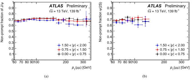
The non-prompt production fractions for

J/ψ

and

ψ(

2S

)

are presented in Figure 5. Note that the

p_T

- dependence of prompt and non-prompt contributions in the

p_T

range covered by this measurement is similar, resulting in the non-prompt fractions being close to constant, for both

J/ψ

and

ψ(

2S

)

.

Finally, the production ratios of

ψ(

2S

)

relative to

J/ψ

are presented in Figure 6, separately for prompt (a) and non-prompt (b) production mechanisms.

A comparison of these results with the predictions of the FONLL model [1, 2] obtained using the web-based

tool [27] with default parameters, is shown in Figure 7. The comparison gives good agreement at the

lower

p_T

, but with FONLL predicting somewhat higher cross-sections at high-

p_T

.

(9)

70 100 200 300 ) [GeV]

µ µ

T( p 1

10 102

Fractional Uncertainty [%]

ATLAS Preliminary

= 13 TeV, 139 fb-1

s

| < 0.75 y 0.00 < |

Differential prompt cross-section ψ

J/

Total Uncertainty Total Systematics

Statistical Fit Model Muon Reco Trigger Bin Migration

(a)

70 100 200 300

) [GeV]

µ µ

T( p 1

10 102

= 13 TeV, 139 fb-1

s

| < 0.75 y 0.00 < |

Differential non-prompt cross-section ψ

J/

(b)

70 100 200 300

) [GeV]

µ µ

T( p 1

10 102

= 13 TeV, 139 fb-1

s

| < 0.75 y 0.00 < |

Differential prompt (2S) cross-section ψ

(c)

70 100 200 300

) [GeV]

µ µ

T( p 1

10 102

= 13 TeV, 139 fb-1

s

| < 0.75 y 0.00 < |

Differential non-prompt (2S) cross-section ψ

(d)

Figure 2: The total, statistical, and systematic fractional uncertainties are shown as a function ofp_Tfor (a) prompt J/ψ, (b) non-promptJ/ψ, (c) promptψ(2S), (d) non-promptψ(2S)mesons for the rapidity slice|y|<0.75. The main components of the systematic uncertainties are also shown.

(10)

60 70 80 90100 200 300 ) [GeV]

µ µ

T( p

−2

10

−1

10 1 10 102

103

104

105

[fb/GeV] yd Tpdσ2 d) -µ+µ→ψBr(J/

s

ψ Prompt J/

| < 2.00 y , 1.50 < | 102

× data

| < 1.50 y , 0.75 < | 101

× data

| < 0.75 y , 0.00 < | 100

× data

(a)

60 70 80 90100 200 300

) [GeV]

µ µ

T( p

−2

10

−1

10 1 10 102

103

104

105

[fb/GeV] yd Tpdσ2 d) -µ+µ→ψBr(J/

s

ψ Non-prompt J/

| < 2.00 y , 1.50 < | 102

× data

| < 1.50 y , 0.75 < | 101

× data

| < 0.75 y , 0.00 < | 100

× data

(b)

Figure 3: Differential cross sections of prompt (a) and non-prompt (b) production ofJ/ψmesons. A scaling factor of 1,10,100 is applied for visual clarity to the rapidity slices|y|<0.75, 0.75<|y|<1.5, 1.5<|y|<2.0, respectively.

For each data point, the horizontal bar spans thep_Trange covered by that bin, with the vertical uncertainty (obscured behind the marker for some values) combining both the statistical (with a bar), and the combined total uncertainty.

The horizontal position of each point represents the mean of the weightedp_Tdistribution for that bin.

60 70 80 90100 200 300

) [GeV]

µ µ

T( p

−1

10 1 10 102

103

104

[fb/GeV] yd Tpdσ2 d) -µ+ µ→(2S)ψBr(

s

ψ(2S) Prompt

| < 2.00 y , 1.50 < | 102

× data

| < 1.50 y , 0.75 < | 101

× data

| < 0.75 y , 0.00 < | 100

× data

(a)

60 70 80 90100 200 300

) [GeV]

µ µ

T( p

−1

10 1 10 102

103

104

[fb/GeV] yd Tpdσ2 d) -µ+ µ→(2S)ψBr(

s

ψ(2S) Non-prompt

| < 2.00 y , 1.50 < | 102

× data

| < 1.50 y , 0.75 < | 101

× data

| < 0.75 y , 0.00 < | 100

× data

(b)

Figure 4: Differential cross sections of prompt (a) and non-prompt (b) production ofψ(2S)mesons. A scaling factor of 1,10,100 is applied for visual clarity to the rapidity slices|y|<0.75, 0.75<|y|<1.5, 1.5<|y|<2.0, respectively.

(11)

60 70 80 90100 200 300 ) [GeV]

µ µ

T( p 0

0.1 0.2 0.3 0.4 0.5 0.6 0.7 0.8 0.9 Non-prompt fraction of J/ψ 1

ATLAS Preliminary

= 13 TeV, 139 fb-1

s

| < 2.00 y 1.50 < |

| < 1.50 y 0.75 < |

| < 0.75 y 0.00 < |

(a)

60 70 80 90100 200 300

) [GeV]

µ µ

T( p 0

0.1 0.2 0.3 0.4 0.5 0.6 0.7 0.8 0.9 1

(2S)ψNon-prompt fraction

= 13 TeV, 139 fb-1

s

| < 2.00 y 1.50 < |

| < 1.50 y 0.75 < |

| < 0.75 y 0.00 < |

(b)

Figure 5: Non-prompt production fraction of (a)J/ψand (b)ψ(2S)after all relevant corrections are applied. The range of results for (b)ψ(2S)is shown up to 140 GeV, covering bins with sufficient statistics for a reliable measurement.

60 70 80 90100 200 300

) [GeV]

µ µ

T( p 0

0.02 0.04 0.06 0.08 0.1 0.12 0.14

Prompt production ratio

= 13 TeV, 139 fb-1

s

| < 2.00 y 1.50 < |

| < 1.50 y 0.75 < |

| < 0.75 y 0.00 < |

(a)

60 70 80 90100 200 300

) [GeV]

µ µ

T( p 0

0.02 0.04 0.06 0.08 0.1 0.12 0.14

Non-prompt production ratio

= 13 TeV, 139 fb-1

s

| < 2.00 y 1.50 < |

| < 1.50 y 0.75 < |

| < 0.75 y 0.00 < |

(b)

Figure 6: Ratio ofψ(2S)production with respect toJ/ψ, for (a) prompt and (b) non-prompt production mechanisms after all relevant corrections are applied. The range of results shown is up to 140 GeV, covering bins with sufficient statistics for a reliable measurement. For each data point, the horizontal bar spans thep_Trange covered by that bin, with the vertical uncertainty (obscured behind the marker for some values) combining both the statistical (with a bar), and the combined total uncertainty. The horizontal position of each point represents the mean of the weightedp_T distribution for that bin. The data are shown after all relevant corrections are applied.

(12)

60 70 80 90100 200 300 ) [GeV]

µ µ

T( p

−2

10

−1

10 1 10 102

103

104

105

[fb/GeV] yd Tpdσ2d) -µ+µ→ψBr(J/

ATLAS Preliminary Cross-Section ψ

Non-prompt J/

| < 2.00 y , 1.50 < | 102

× data

| < 1.50 y , 0.75 < | 101

× data

| < 0.75 y , 0.00 < | 100

× data FONLL

(a)

60 70 80 90100 200 300

) [GeV]

µ µ

T( p

−1

10 1 10 102

103

[fb/GeV] ydTpdσ2d) -µ+µ→(2S)ψBr(

ATLAS Preliminary (2S) Cross-Section ψ

Non-prompt

| < 2.00 y , 1.50 < | 102

× data

| < 1.50 y , 0.75 < | 101

× data

| < 0.75 y , 0.00 < | 100

× data

FONLL

(b)

= 13 TeV, 139 fb-1

s

Cross-Section Non-prompt J/ψ

| < 2.00 y 1.50 < |

| < 1.50 y 0.75 < |

| < 0.75 y 0.00 < | FONLL

60 70 80 90 100 200 300

) [GeV]

µ (µ pT 0.5

1 1.5 2 2.5

3⁶⁰ ⁷⁰ ⁸⁰ ^{90 100} ²⁰⁰ ₍_µ³⁰⁰_µ_{) [GeV]}

pT 0.5

1 1.5 2 2.5

360 70 80 90 100 200 300

) [GeV]

µ µ T( p 0.5

1 1.5 2 2.5 3

Theory / Data

/ Data

(c)

= 13 TeV, 139 fb-1

s

(2S) Cross-Section Non-prompt ψ

| < 2.00 y 1.50 < |

| < 1.50 y 0.75 < |

| < 0.75 y 0.00 < | FONLL

60 70 80 90 100 200 300

) [GeV]

µ (µ pT 0.6

0.8 1 1.2

1.4⁶⁰ ⁷⁰ ⁸⁰ ^{90 100} ²⁰⁰ ₍_µ³⁰⁰_µ_{) [GeV]}

pT 0.6

0.8 1 1.2

1.460 70 80 90 100 200 300

) [GeV]

µ µ T( p 0.6

0.8 1 1.2 1.4

Theory / Data

/ Data

(d)

Figure 7: The non-prompt differential cross-section overlaid with FONLL [27] predictions are shown for (a)J/ψ mesons, and (b)ψ(2S)mesons, where the horizontal position of each point represents the mean of the weighted p_Tdistribution for that bin. The data are shown after all relevant corrections are applied, including corrections for acceptance under an isotropic assumption. The ratios of the FONLL prediction to the measured differential cross-sections are shown for non-prompt (c)J/ψand (d)ψ(2S)mesons. The green shaded bands represent the range of theoretical uncertainty associated to the variations of the scales. The symbols for the data are centred at unity and the vertical error bars represent the relative uncertainties of the data.

(13)

6 Summary

This note describes the results of a measurement of the double-differential production cross-section of

J/ψ

and

ψ(

2S

)

charmonium states through their decays to dimuons in

pp

collisions at

√s =

13 TeV, performed using the data collected by the ATLAS detector at the LHC during Run 2. For each of the two states, the cross-sections are measured separately for prompt and non-prompt production mechanisms. The non-prompt fractions for each state are also measured, as well as the production ratios of

ψ(

2S

)

to

J/ψ

. In case of

J/ψ

, the results cover the rapidity range

|y| <

2 and the transverse momentum range between 60 GeV and 360 GeV. In case of

ψ(

2S

)

the rapidity range is the same, but the transverse momentum range is between 60 GeV and 140 GeV. In both cases, the transverse momentum range goes well beyond the values reached so far, which may help discriminate various theoretical models.

The results show similar

p_T

-dependence for prompt and non-prompt differential cross sections, with

non-prompt fractions close to constant for both

J/ψ

and

ψ(

2S

)

in this range of transverse momenta. The

results for non-prompt production are compared with the predictions of the FONLL model with default set

of parameters. These predictions are consistent with the present measurement at the low end of the

p_T

range, but exceed the experimental values at large transverse momenta.

(14)

Appendix

The acceptance for

ψ

mesons depends on their spin-alignment. The nominal results presented in this paper assume a flat angular distribution, corresponding to the unpolarised case. In order to assess the dependence of the cross section on the spin-alignment, the acceptance maps were reweighted for a variety of spin-alignment scenarios, and correction factors for each analysis bin were determined with respect to the nominal values. It was found that the correction factors for

J/ψ

and

ψ(

2S

)

are the same within

<

1%.

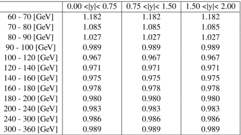
The correction factors for longitudinal and transverse spin-alignment (defined in the helicity frame of the charmonium state) are shown in tables 2 and 3 respectively. These were found to be the largest among the various scenarios considered. The correction factors for different variants of transverse polarisation were found to be the same within

<

1%.

0.00 <|y|< 0.75 0.75 <|y|< 1.50 1.50 <|y|< 2.00

60 - 70 [GeV] 0.623 0.624 0.623

70 - 80 [GeV] 0.826 0.826 0.826

80 - 90 [GeV] 0.946 0.946 0.946

90 - 100 [GeV] 1.020 1.020 1.020

100 - 120 [GeV] 1.065 1.065 1.065

120 - 140 [GeV] 1.058 1.058 1.058

140 - 160 [GeV] 1.050 1.050 1.050

160 - 180 [GeV] 1.044 1.044 1.044

180 - 200 [GeV] 1.040 1.040 1.040

200 - 240 [GeV] 1.034 1.034 1.034

240 - 300 [GeV] 1.028 1.028 1.028

300 - 360 [GeV] 1.022 1.022 1.022

Table 2: Mean weight correction factor forJ/ψunder the "longitudinal" spin-alignment hypothesis.

0.00 <|y|< 0.75 0.75 <|y|< 1.50 1.50 <|y|< 2.00

60 - 70 [GeV] 1.182 1.182 1.182

70 - 80 [GeV] 1.085 1.085 1.085

80 - 90 [GeV] 1.027 1.027 1.027

90 - 100 [GeV] 0.989 0.989 0.989

100 - 120 [GeV] 0.967 0.967 0.967

120 - 140 [GeV] 0.971 0.971 0.971

140 - 160 [GeV] 0.975 0.975 0.975

160 - 180 [GeV] 0.978 0.978 0.978

180 - 200 [GeV] 0.980 0.980 0.980

200 - 240 [GeV] 0.983 0.983 0.983

240 - 300 [GeV] 0.986 0.986 0.986

300 - 360 [GeV] 0.989 0.989 0.989

Table 3: Mean weight correction factor forJ/ψunder "transverse" spin-alignment hypotheses.

(15)

References

[1] M. Cacciari, S. Frixione and P. Nason, The p(T) spectrum in heavy flavor photoproduction , JHEP

0103

(2001) 006, arXiv: hep-ph/0102134 [hep-ph] (cit. on pp. 2, 8).

[2] M. Cacciari, S. Frixione, N. Houdeau, M. L. Mangano, P. Nason et al., Theoretical predictions for charm and bottom production at the LHC , JHEP

1210

(2012) 137, arXiv: 1205.6344 [hep-ph]

(cit. on pp. 2, 8).

[3] G. T. Bodwin, E. Braaten and G. P. Lepage, Rigorous QCD analysis of inclusive annihilation and production of heavy quarkonium , Phys. Rev.

D51

(1995) 1125, [Erratum: Phys. Rev.D55,5853(1997)], arXiv: hep-ph/9407339 [hep-ph] (cit. on p. 2).

[4] ATLAS Collaboration, Measurement of the differential cross-sections of prompt and non-prompt production of

J/ψ

and

ψ(

2 S) in

pp

collisions at

√

s =

7 and 8 TeV with the ATLAS detector , Eur.

Phys. J. C

76

(2016) 283, arXiv: 1512.03657 [hep-ex] (cit. on p. 2).

[5] ATLAS Collaboration, Measurement of the production cross-section of

ψ(

2 S) →

J/ψ(→ µ⁺µ⁻)π⁺π⁻

in

pp

collisions at

√

s=

7 TeV at ATLAS , JHEP

09

(2014) 079, arXiv: 1407.5532 [hep-ex] (cit. on p. 2).

[6] LHCb Collaboration, Measurement of

ψ(

2

S)

meson production in

pp

collisions at

√

s=7 TeV

, Eur.

Phys. J.

C72

(2012) 2100, arXiv: 1204.1258 [hep-ex] (cit. on p. 2).

[7] CMS Collaboration,

J/ψ

and

ψ_2S

production in

pp

collisions at

√

s =

7 TeV , JHEP

02

(2012) 011, arXiv: 1111.1557 [hep-ex] (cit. on p. 2).

[8] ALICE Collaboration,

J/ψ

polarization in

pp

collisions at

√

s =

7 TeV , Phys. Rev. Lett.

108

(2012) 082001, arXiv: 1111.1630 [hep-ex] (cit. on p. 2).

[9] CMS Collaboration, Measurement of the prompt

J/ψ

and

ψ(

2 S) polarizations in

pp

collisions at

√s =

7 TeV , Phys. Lett. B

727

(2013) 381, arXiv: 1307.6070 [hep-ex] (cit. on p. 2).

[10] LHCb Collaboration, Measurement of

ψ(

2

S)

polarisation in

pp

collisions at

√

s =

7 TeV , Eur. Phys.

J.

C74

(2014) 2872, arXiv: 1403.1339 [hep-ex] (cit. on p. 2).

[11] ALICE Collaboration, Measurement of the inclusive J/ψ polarization at forward rapidity in pp collisions at

√

s=8

TeV , Eur. Phys. J.

C78

(2018) 562, arXiv: 1805.04374 [hep-ex] (cit. on p. 2).

[12] ATLAS Collaboration, Measurement of the production cross section of prompt

J/ψ

mesons in association with a

W^±

boson in

pp

collisions at

√

s =

7 TeV with the ATLAS detector , JHEP

04

(2014) 172, arXiv: 1401.2831 [hep-ex] (cit. on p. 2).

[13] ATLAS Collaboration, Observation and measurements of the production of prompt and non-prompt

J/ψ

mesons in association with a

Z

boson in

pp

collisions at

√

s

= 8 TeV with the ATLAS detector , Eur. Phys. J.

C75

(2015) 229, arXiv: 1412.6428 [hep-ex] (cit. on p. 2).

[14] G. Li, M. Song, R.-Y. Zhang and W.-G. Ma, QCD corrections to

J/ψ

production in association with a

W-boson at the LHC

, Phys. Rev.

D83

(2011) 014001, arXiv: 1012.3798 [hep-ph] (cit. on p. 2).

[15] J. P. Lansberg and C. Lorce, Reassessing the importance of the colour-singlet contributions to direct

J/ψ+W

production at the LHC and the Tevatron , Phys. Lett.

B726

(2013) 218, [Erratum: Phys.

Lett.B738,529(2014)], arXiv: 1303.5327 [hep-ph] (cit. on p. 2).

[16] B. Gong, J.-P. Lansberg, C. Lorce and J. Wang, Next-to-leading-order QCD corrections to the yields

and polarisations of J/Psi and Upsilon directly produced in association with a Z boson at the LHC ,

JHEP

03

(2013) 115, arXiv: 1210.2430 [hep-ph] (cit. on p. 2).

(16)

[17] M. Song, W.-G. Ma, G. Li, R.-Y. Zhang and L. Guo, QCD corrections to

J/ψ

plus

Z⁰

-boson production at the LHC , JHEP

02

(2011) 071, [Erratum: JHEP12,010(2012)], arXiv: 1102.0398 [hep-ph] (cit. on p. 2).

[18] M. Butenschoen and B. A. Kniehl, J/ψ production in NRQCD: A global analysis of yield and polarization , Nucl. Phys. Proc. Suppl.

222-224

(2012) 151, arXiv: 1201.3862 [hep-ph] (cit. on p. 2).

[19] CMS Collaboration, Measurement of

J/ψ

and

ψ(

2 S) Prompt Double-Differential Cross Sections in

pp

Collisions at

√

s=

7 TeV , Phys. Rev. Lett.

114

(2015) 191802, arXiv: 1502.04155 [hep-ex]

(cit. on p. 2).

[20] CMS Collaboration, Measurement of quarkonium production cross sections in

pp

collisions at

√s =

13 TeV , Phys. Lett. B

780

(2018) 251, arXiv: 1710.11002 [hep-ex] (cit. on p. 2).

[21] ALICE Collaboration, Measurement of quarkonium production at forward rapidity in

pp

collisions at

√

s=

7 TeV , Eur. Phys. J.

C74

(2014) 2974, arXiv: 1403.3648 [nucl-ex] (cit. on p. 2).

[22] ATLAS Collaboration, Measurement of

χ_c1

and

χ_c2

production with

√

s=

7 TeV

pp

collisions at ATLAS , JHEP

07

(2014) 154, arXiv: 1404.7035 [hep-ex] (cit. on p. 2).

[23] ATLAS Collaboration, The ATLAS Experiment at the CERN Large Hadron Collider , JINST

3

(2008) S08003 (cit. on p. 3).

[24] ATLAS Collaboration, Muon reconstruction performance of the ATLAS detector in proton–proton collision data at

√

s =

13 TeV , Eur. Phys. J. C

76

(2016) 292, arXiv: 1603.05598 [hep-ex] (cit. on pp. 3, 4, 7).

[25] ATLAS Collaboration, Luminosity determination in

pp

collisions at

√

s=

13 TeV using the ATLAS detector at the LHC , ATLAS-CONF-2019-021, 2019, url: http://cds.cern.ch/record/

2677054 (cit. on p. 8).

[26] G. Avoni et al., The new LUCID-2 detector for luminosity measurement and monitoring in ATLAS , JINST

13