ATLAS-CONF-2014-040 05July2014
ATLAS NOTE
ATLAS-CONF-2014-040
July 2, 2014
Measurement of the total cross section from elastic scattering in pp collisions at √
s = 7 TeV with the ATLAS detector
The ATLAS Collaboration
Abstract
In this paper a measurement of the total pp cross section at the LHC at
√s
=7 TeV is presented. In a special run with high
β⋆beam optics, an integrated luminosity of 80
µb−1was accumulated in order to measure the differential elastic cross section as a function of the Mandelstam momentum transfer variable t. The measurement is performed in the range from
−t
=0.0025 GeV
2to
−t
=0.38 GeV
2, with the ALFA sub-detector of ATLAS. From the extrapolation of the elastic t-spectrum to
|t
| →0, the total cross section
σtot(pp
→X) is measured using the optical theorem to be
σtot
( pp
→X)
=95.35
±0.38 (stat.)
±1.25 (exp.)
±0.37 (extr.) mb
,where the first error is statistical, the second accounts for all experimental systematic uncer- tainties and the last is related to uncertainties on the extrapolation to
|t
| →0. In addition, the slope of the elastic cross section at small
|t
|is determined to be B
=19.73
±0.14 (stat.)
±0.26 (syst.) GeV
−2.
c Copyright 2014 CERN for the benefit of the ATLAS Collaboration.
Reproduction of this article or parts of it is allowed as specified in the CC-BY-3.0 license.
1 Introduction
The total hadronic cross section is a fundamental parameter in strong interactions, setting the scale of the size of the interaction region at a given energy. A first principle calculation of the total hadronic cross section based upon quantum chromodynamics (QCD) is not possible. Large distances are involved in the collision process and thus perturbation theory is not applicable. Even though the total cross section cannot be directly calculated, it can be estimated or bound by a number of fundamental relations in high energy scattering theory which are model independent. The Froissart–Martin bound [1, 2], which states that the total cross section cannot grow asymptotically faster than ln
2s,
√s being the centre-of- mass energy, is based upon principles of axiomatic field theory. The optical theorem, which relates the imaginary part of the forward elastic amplitude to the total cross section, is a general theorem in quantum scattering theory. Dispersion relations, which connect the real part of the elastic-scattering amplitude to an integral of the total cross section over energy, are based upon the analyticity and crossing symmetry of the scattering amplitude. All of these relations lead to testable constraints on the total cross section.
The rise of the pp cross section with energy was first observed at the ISR [3, 4]. The fact that the hadronic cross section continues to rise has been confirmed in every new energy regime made accessi- ble by a new pp or p p ¯ collider (Sp¯pS, Tevatron and LHC) [5–11]. However, the “asymptotic” energy dependence is yet to be determined. Does the cross section rise with a ln
2s dependence to saturate the Froissart–Martin bound, or is there rather a ln s dependence? These are questions that are still being addressed.
Traditionally, the total cross section at hadron colliders has been measured via elastic scattering using the optical theorem. This paper presents a measurement by the ATLAS experiment [12] at the LHC in
pp collisions at
√s
=7 TeV using this approach. The optical theorem states:
σtot∝
Im [ f
el(t
→0)] (1)
where f
el(t
→0) is the elastic-scattering amplitude extrapolated to the forward direction, i.e. at
|t
| →0, t being the four-momentum transfer. Thus, a measurement of elastic scattering in the very forward direction gives information on the total cross section. It requires an independent measurement of the luminosity. In this analysis the luminosity is determined from LHC beam parameters using van der Meer scans [13]. Once the luminosity is known, the elastic cross section can be normalized. An extrapolation of the differential cross section to
|t
| →0 gives the total cross section through the formula:
σ2tot=
16π(
~c)
21
+ρ2dσ
eldt
t→0
,
(2)
where
ρrepresents a small correction arising from the ratio of the real to imaginary part of the elastic- scattering amplitude in the forward direction and is taken from theory.
In order to minimize the model dependence in the extrapolation to
|t
| →0, the elastic cross section has to be measured down to as small
|t
|values as possible. In this analysis elastic scattering is measured in the range 0.0025 GeV
2 < −t
<0.38 GeV
2. This also allows measurements of the nuclear slope parameter B, which describes the exponential t-dependence of the nuclear amplitude at small t-values. In a simple geometrical model of elastic scattering, B is related to the size of the proton and thus its energy dependence is strongly correlated with that of the total cross section.
The measurements of the total cross section and elastic scattering reported here are used to determine
the inelastic cross section, as the difference between these two quantities. This measurement of the
inelastic cross section is compared with a previous measurement of the ATLAS experiment using a
complementary method, based upon data from a minimum bias trigger [14]. The ratio of the elastic to the
total cross section is also derived. In the black disc limit (i.e. the limit in which the proton is completely
opaque) this quantity goes asymptotically to 0.5 and thus the measurement is directly sensitive to the
hadron opacity. The quantities measured and reported here have also been measured at the LHC by the TOTEM experiment [15, 16].
This paper is organised as follows. The experimental setup including a brief description of the
ALFA sub-detector is given in Section 2, followed by a short description of the measurement method in
Section 3. Section 4 summarises theoretical predictions and Monte Carlo simulation. The data taking
and trigger conditions are outlined in Section 5, followed by a description of the track reconstruction
and alignment procedures in Section 6. The data analysis consisting of event selection, background
determination and reconstruction efficiency is explained in Section 7. Section 8 describes the acceptance
and unfolding corrections. The determination of the beam optics is summarised in Section 9 and of the
luminosity in Section 10. Results for the differential elastic cross section are reported in Section 11 and
the extraction of the total cross section in Section 12. The results are discussed in Section 13 with a
summary in Section 14.
2 Experimental setup
ATLAS is a multi-purpose detector designed to study elementary processes in proton–proton interactions at the TeV energy scale. It consists of an inner tracking system, calorimeters and a muon spectrometer surrounding the interaction point of the colliding beams. The tracking system covers the pseudorapidity range
|η| <2.5 and the calorimetric measurements range to
|η| =4.9.
1To improve the coverage in the forward direction three smaller detectors with specialised tasks are installed at large distance from the interaction point. The most forward detector, ALFA, is sensitive to particles in the range
|η| >8.5, while the two others have acceptance windows at
|η| ≈5.8 (LUCID) and
|η| ≈8.2 (ZDC). A detailed description of the ATLAS detector can be found in Ref. [12].
The ALFA detector (Absolute Luminosity For ATLAS) is designed to measure small-angle proton scattering. Two tracking stations are placed on either side of the central ATLAS detector at distances of 238 m and 241 m from the interaction point. The tracking detectors are housed in so-called Roman Pots (RPs) which can be moved in close to the circulating proton beams. Combined with a special beam optics, as introduced in Section 3, this allows the detection of protons at scattering angles of 10
µrad.Each station carries an upper and lower RP which is connected by flexible bellows to the primary LHC vacuum. The RPs are made of stainless steel with thin windows of 0.2 mm and 0.5 mm thickness at the bottom and front sides to reduce the interactions of traversing protons. Elastically scattered protons are detected in the main detectors (MDs) while dedicated overlap detectors (ODs) measure the distance between upper and lower MDs. The arrangement of the upper and lower MDs and ODs with respect to the beam is illustrated in Fig. 1.
Figure 1: A schematic view of a pair of ALFA tracking detectors in the upper and lower RPs. The distance between the two MDs is measured using particles which pass through both ODs on either side of each MD. Although not shown in the figure, the ODs are mechanically attached to the MDs.
Each MD consists of 2 times 10 layers of 64 square scintillating fibres with 0.5 mm side length glued on titanium plates. The fibres on the front and back sides of each titanium plate are orthogonally arranged at angles of
±45
◦with respect to the vertical
y-axis. The projections perpendicular to the fibreaxes define the u and
vcoordinates which are used in the track reconstruction described in Section 6.1.
1ATLAS uses a right-handed coordinate system with its origin at the nominal. interaction point in the centre of the detector and thez-axis along the beam pipe. Thex-axis points from the interaction point to the centre of the LHC ring and they-axis points upwards The pseudorapidityηis defined in terms of the polar angleθasη=−ln tan(θ/2).
To minimise optical cross-talk each fibre is coated with a thin aluminium film. The individual fibre layers are staggered by multiples of 1/10 of the fibre size to improve the position resolution. The theoretical resolution of 14.4
µm peru or
vcoordinate is degraded due to imperfect staggering, cross-talk, noise and inefficient fibre channels. To reduce the impact of imperfect staggering on the detector resolution, all fibre positions were measured by microscope. In a test beam [17, 18] with 120 GeV hadrons, the position resolution was measured to be between 30
µm and 35µm. The efficiency to detect a traversingproton in a single fibre layer is typically 93%, with layer to layer variations of about 1%. The overlap detectors consist of three layers of 30 scintillating fibres per layer measuring the vertical coordinate of traversing beam halo particles or shower fragments.
2Two independent ODs are attached at each side of both MDs, as sketched in Fig. 1. The alignment of the ODs with respect to the coordinate system of the MDs was performed by test beam measurements using a Silicon pixel telescope. A staggering by 1/3 of the fibre size results in a single-track resolution of about 50
µm. The signals from both types of trackingdetectors are amplified by 64-channel multi-anode photo-multipliers (MAPMTs). The scintillating fibres are directly coupled to the MAPMT photo-cathode. Altogether, 23 MAPMTs are used to read out each MD and its two adjacent ODs.
Both tracking detectors are completed by trigger counters which consist of 3 mm thick scintillator plates covering the active areas of MDs and ODs. Each MD is equipped with two trigger counters and their signals are used in coincidence to reduce noise contributions. The ODs are covered by single trigger counters and each signal is recorded. Clear-fibre bundles are used to guide all scintillation signals from the trigger counters to single channel photo-multipliers.
Before data taking, precision motors move the RPs vertically in 5
µm steps towards the beam. Theposition measurement is realised by inductive displacement sensors (LVDT) which were calibrated by a laser survey in the LHC tunnel. The internal precision of these sensors is 10
µm. In addition, the motorsteps are used to cross-check the LVDT values.
The compact front-end electronics is assembled in a three-layer structure which is attached to the back side of each MAPMT. The three layers comprise a high-voltage divider board, a passive board for signal routing and an active board for signal amplification, discrimination and buffering using the MAROC chip [19, 20]. The buffers of all 23 MAPMT readout chips of a complete detector are serially transmitted by five kapton cables to the mother-board. All digital signals are transmitted via a fibre optical link to the central ATLAS data acquisition system. The analogue trigger signals are sent by fast air-core cables to the central trigger processor.
The station and detector naming scheme is depicted in Fig. 2. The stations A7R1 and B7R1 are positioned at z
=−237.4 m and z
=−241.5 m respectively in the outgoing beam 1 (C side), while the stations A7L1 and B7L1 are situated symmetrically in the outgoing beam 2 (A side). The detectors A1–A8 are inserted in increasing order in stations B7L1, A7L1, A7R1 and B7R1 with even-numbered detectors in the lower RPs. Two spectrometer arms for elastic-scattering event topologies are defined by the following detector series: arm 1 comprising detectors A1, A3, A6, A8, and arm 2 comprising detectors A2, A4, A5, A7. The sequence of quadrupoles between the interaction point and ALFA is also shown in Fig. 2. Among them, the inner triplet Q1–Q3 is most important for the high-β
⋆beam optics necessary for this measurement.
2Halo particles originate from beam particles which left the bunch structure of the beam but still circulate in the beam pipe.
Figure 2: A sketch of the experimental set-up, not to scale, showing the positions of the ALFA Roman
Pot stations in the outgoing LHC beams, and the quadrupole (Q1–Q6) and dipole (D1–D2) magnets
situated between the interaction point and ALFA. The ALFA detectors are numbered A1–A8, and are
combined into inner stations A7R1 and A7L1, which are closer to the interaction point, and outer stations
B7R1 and B7L1. The arrows indicate in the top panel the beam directions and in the bottom panel the
scattered proton directions.
3 Measurement method
The data were recorded with a special beam optics with a
β⋆of 90 m [21, 22] at the interaction point resulting in a small divergence and providing a parallel-to-point focusing in the vertical plane.
3In a parallel-to-point beam optics the betatron oscillation has a phase advance
Ψof 90
◦between the interac- tion point and the Roman Pots, such that all particles scattered at the same angle are focused at the same position at the detector, independent of their production vertex position. This focusing is only achieved in the vertical plane.
The beam optics parameters are needed for the reconstruction of the scattering angle
θ⋆at the inter- action point. The four-momentum transfer t is calculated from
θ⋆; in elastic scattering at high energies this is given by:
−
t
=θ⋆×
p
2,
(3)
where p is the nominal beam momentum of the LHC of 3.5 TeV and
θ⋆is measured from the proton trajectories in ALFA. A formalism based on transport matrices allows positions and angles of particles at two different points of the magnetic lattice to be related.
The trajectory (u(z),
θu(z)), where u
=x, y is the transverse position with respect to the nominal orbit at a distance z from the interaction point and
θuis the angle between u and z, is given by the transport matrix
Mand the coordinates at the interaction point (u
⋆,
θ⋆u):
u(z)
θu(z)
!
=M
u
⋆ θ⋆u!
=
M
11M
12M
21M
22!
u
⋆ θu⋆!
,
(4)
where the elements of the transport matrix can be calculated from the optical function
β, its derivativewith respect to z and
Ψ. Mmust be calculated separately in x and
yand depends on the longitudinal position z; the corresponding indices have been dropped for clarity. While the focussing properties of the beam optics in the vertical plane enable a reconstruction of the scattering using only M
12with a good precision, the phase advance in the horizontal plane is close to 180
◦and different reconstruction methods are investigated.
The ALFA detector was designed to use the “subtraction” method, exploiting the fact that for elas- tic scattering the particles are back-to-back, the scattering angle at the A- and C-side are the same in magnitude and opposite in sign, and the protons originate from the same vertex. The beam optics was optimized to maximize the lever arm M
12in the vertical plane in order to access the smallest possi- ble scattering angle. The positions measured with ALFA at the A- and C-side of ATLAS are roughly of the same modulus but opposite sign and in the subtraction method the scattering angle is calculated according to:
θ⋆u =
u
A−u
CM
12,A+M
12,C .(5)
This is the nominal method in both planes and yields the best t-resolution. An alternative method for the reconstruction of the horizontal scattering angle is to use the “local angle”
θumeasured by the two detectors on the same side :
θ⋆u = θu,A−θu,C
M
22,A+M
22,C.
(6)
Another method performs a “local subtraction” of measurements at the inner station at 237 m and the outer station at 241 m, separately at the A- and C-side, before combining the two sides:
θ⋆u,S =
M
24111,S ×u
237,S −M
23711,S ×u
241,SM
11,S241 ×M
12,S237 −M
23711,S ×M
12,S241 ,S
=A, C
.(7)
3Theβ-function determines the variation of the beam envelope around the ring and depends on the focusing properties of the magnetic lattice.
Finally, the “lattice” method uses both the measured positions and the local angle to reconstruct the scattering angle by the inversion of the transport matrix
u
⋆ θ⋆u!
=M−1
u
θu!
,
(8)
and from the second row of the inverted matrix the scattering angle is determined
θ⋆u =
M
12−1×u
+M
22−1×θu .(9) All methods using the local angle suffer from a poor resolution due to a moderate angular resolution of about 10
µrad. Nevertheless, the alternative methods are used to cross check the subtraction method anddetermine beam optics parameters.
For all methods the t is calculated from the scattering angles as follows:
−
t
=(θ
⋆x)
2+(θ
⋆y)
2p
2 ,(10)
where
θ⋆yis always reconstructed with the subtraction method, because of the parallel-to-point focusing
in the vertical plane, and four different methods are used for
θ⋆x. Results on
σtotusing the four methods
will be discussed in Section 12.
4 Theoretical prediction and Monte Carlo simulation
Elastic scattering is related to the total cross section through the optical theorem Eq. (1) and the differen- tial elastic cross section is obtained from the scattering amplitudes of the contributing diagrams:
dσ dt
=1
16π
f
N(t)
+f
C(t)e
iαφ(t)2 .
(11)
Here, f
Nis the purely strongly interacting amplitude, f
Cis the Coulomb amplitude and a phase
φis induced by long-range Coulomb interactions [23, 24]. The individual amplitudes are given by
f
C(t)
= −8πα
~c G
2(t)
t
,(12)
f
N(t)
=(ρ
+i)
σtot~
c e
−Bt/2 ,(13)
where G is the electric form factor of the proton, B the nuclear slope and
ρ =Re( f
el)/Im( f
el). The expression for the nuclear amplitude f
Nis an approximation valid at small
|t
|only. This analysis uses the calculation of the Coulomb phase from Ref. [24] with a conventional dipole parameterization of the proton electric form factor from Ref. [25]. The theoretical form of the t-dependence of the cross section is obtained from the evaluation of the square of the complex amplitudes:
dσ
dt
=4πα
2(
~c)
2|
t
|2 ×G
4(t) (14)
− σtot×αG2
(t)
|
t
|sin (αφ(t))
+ρcos (αφ(t))
×
exp
−B
|t
|2
+ σ2tot1
+ρ216π(
~c)
2 ×exp (
−B
|t
|)
,where the first term corresponds to the Coulomb interaction, the second to the Coulomb-nuclear interfer- ence and the last to the hadronic interaction. The inclusion of Coulomb interaction in the fit of the total cross section increases the value of
σtotby about 0.6 mb, compared with a fit with the nuclear term only.
This parameterization is used to fit the differential elastic cross section to extract
σtotand B. The value of
ρis extracted from global fits performed by the COMPETE collaboration to lower energy elas- tic scattering data comprising results from a variety of initial states [26, 27]. Systematic uncertainties originating from the choice of model are important and are addressed e.g. in Ref. [28]. Additionally, the inclusion of different data sets in the fit influences the value of
ρ, as described in Refs. [29,30]. In this pa-per the value from Ref. [26] is used with a conservative estimate of the systematic uncertainty to account for the model dependence:
ρ =0.140
±0.008. The theoretical prediction Eq. (14) depends also on the Coulomb phase
φand the form factor G. Uncertainties in the Coulomb phase are estimated by replacing the simple parameterization from Ref. [24] with alternative calculations from Refs. [25] and [31], which both predict a different t-dependence of the phase. Changing this has only a minor fractional impact of order 10
−4on the cross section prediction.
The uncertainty on the electric form factor is derived from a comparison of the simple dipole param- eterization used in this analysis to more sophisticated forms [32], which describe high-precision low- energy elastic electron-proton data better [33]. Replacing the dipole by other forms also has a negligible impact of order 10
−4on the total cross-section determination.
Alternative parameterizations of the nuclear amplitude which deviate from the simple exponential
t-dependence are discussed in Section 12.3.
4.1 Monte Carlo simulation
Monte Carlo simulated events are used to calculate acceptance and unfolding corrections. The generation of elastic scattering events is performed with PYTHIA8 [34, 35] version 8.165, in which the t-spectrum is generated according to Eq. (14). The divergence of incoming beams and the vertex spread are set in the simulation according to the measurements described in Section 5. After event generation, the elastically scattered protons are transported from the interaction point to the Roman Pots, either by means of the transport matrix Eq. (4) or by the polymorphic tracking code module for the symplectic thick-lens tracking implemented in the MadX [36] beam optics calculation package.
A fast parameterization of the detector response is used for the detector simulation with the detector resolution tuned to the measured resolution. The resolution is measured by extrapolating tracks recon- structed in the inner stations to the outer stations using beam optics matrix-element ratios and comparing predicted positions with measured positions. It is thus a convolution of the resolutions in the inner and outer stations. The fast simulation is tuned to reproduce this convolved resolution.
A full GEANT4 [37, 38] simulation is used to set the resolution scale between detectors at the inner
and outer stations, which cannot be determined from the data. The resolution of the detectors at the outer
stations is slightly worse than for the detectors at the inner stations as multiple scattering and shower
fragments from the latter degrade the performance of the former. Systematic uncertainties from the
resolution difference between the detectors at inner and outer stations are assessed by fixing the resolution
of the detectors at the inner stations either to the value from GEANT4 or to the measurement from the
test beam [17, 18] and matching the resolution at the outer stations to reproduce the measured convolved
resolution. The resolution depends slightly on the vertical track position on the detector surface; a further
systematic uncertainty is derived by replacing the constant resolution by a linear parameterization. The
total systematic uncertainty on the resolution of about
±10% is dominated by the difference between the
value from the test beam measurement and from GEANT4 simulation.
5 Data taking
5.1 Beam conditions
5.1.1 Filling scheme and beam-based alignment
The data were recorded in a dedicated low-luminosity run using beam optics with a
β⋆of 90 m; details of the beam optics settings can be found in Refs. [21, 22]. The duration of this run was four hours. For elastic-scattering events the main pair of colliding bunches was used, which contained around 7
×10
10protons per bunch. Several pairs of pilot bunches with lower intensity and unpaired bunches were used for the studies of systematic uncertainties. The rates of the head-on collisions were maximised using measurements of online luminosity monitors.
A very precise positioning of the Roman Pots is mandatory to achieve the desired precision on the position measurement of typically 20–30
µm in both the horizontal and vertical dimensions. The firststep is a beam-based alignment procedure. This is a procedure to determine the position of the RPs with respect to the proton beams. One at a time, the eight pots are moved into the beam (at the very end by steps of 10
µm only) until the LHC beam-loss monitors give a signal well above threshold. The beam-based alignment procedure was performed in a dedicated fill with identical beam settings just before the data taking run. The eight positions of the vertical beam edges, upper and lower, in the reference system of the four stations were determined.
From the positions of the upper and the lower Roman Pot windows with respect to the beam edges, the centre of the beam as well as the distance between the upper and lower pots were computed. For the two stations on side C the centres were off zero by typically 0.5 to 0.6 mm (for side A by
−0.2 mm). On each side, the distances between the upper and the lower pots were measured to be 8.7 mm for the station nearer to the interaction point and 7.8 mm for the far one. This difference corresponds to the change in the nominal vertical beam widths (σ
y) between the two stations.
The data were collected with the pots at 6.5
×σyfrom the beam centre, the closest possible distance with reasonable background rates. With a value of the nominal vertical beam spread,
σy, of 897
µm(856
µm) for the inner (outer) stations, the 6.5×σypositions correspond to a typical distance of 5.83 mm (5.56 mm) from the beam line in the LHC reference frame.
5.1.2 Beam characteristics: stability and emittance
Beam position monitors, regularly distributed along the beam line between the interaction point and the RPs, were used to survey the horizontal and vertical positions of the beams. The variations in position throughout the duration of data-taking were of the order of 10
µm in both directions, which is equal tothe precision of the measurement itself.
The vertical and horizontal beam emittances
ǫyand
ǫx, expressed in
µm, are used in the simulation toproperly track a scattered proton going from the interaction point to the RPs and therefore to determine the acceptance. These were measured at regular intervals during the fill using a wire-scan method [39]
and monitored bunch-by-bunch throughout the run using two beam synchrotron radiation monitor sys-
tems; the latter were calibrated to the wire-scan measurements at the start of the run. The emittances
varied smoothly from 2.2
µm to 3.0µm (3.2µm to 4.2µm) for beam 1 (beam 2) in the horizontal planeand from 1.9
µm to 2.2µm (2.0µm to 2.2µm) for beam 1 (beam 2) in the vertical plane. The system-atic uncertainty on the emittance is about 10%. A luminosity-weighted average emittance is used in the
simulation resulting in an angular beam divergence of about 3
µrad.5.2 Trigger conditions
To trigger on elastic-scattering events, two main triggers were used. The first required a coincidence
of the main detector trigger scintillators between either of the two upper detectors on side A and either
of the two lower detectors on side C and the second required a coincidence between either of the two
lower detectors on side A and either of the two upper detectors on side C. The elastic-scattering rate was
typically 50 Hz in each arm. The trigger efficiency for elastic-scattering events was determined from a
data stream in which all events with a hit in any one of the ALFA trigger counters were recorded. In
the geometrical acceptance of the detectors, the efficiency of the trigger used to record elastic-scattering
events is 99.96
±0.01%.
6 Track reconstruction and alignment
6.1 Track reconstruction
The reconstruction of elastic scattering events is based on local tracks of the proton trajectory in the RP stations. A well-reconstructed elastic scattering event consists of local tracks in all four RP stations.
The local tracks in the MDs are reconstructed from the hit pattern of traversing protons in the scin- tillating fibre layers. In each MD, 20 layers of scintillating fibres are arranged perpendicular to the beam direction. The hit pattern of elastic protons is characterised by a straight trajectory, almost parallel to the beam direction. In elastic events the average multiplicity per detector is about 23 hits, where typically 18–19 are attributed to the proton trajectory while the remaining 4–5 hits are due to background.
The reconstruction assumes that the protons pass through the fibre detector perpendicularly. A small angle below 1 mrad with respect to the beam direction has no sizable impact. The first step of the reconstruction is to determine the u and
vcoordinates from the two-times-ten layers which have the same orientation. The best estimate of the track position is given by the overlap region of the fiducial areas of all hit fibres. As illustrated in Fig. 3, the staggering of the fibres narrows the overlap region and thereby improves the resolution. The centre of the overlap region gives the u or
vcoordinate, while the width determines the resolution. Pairs of u and
vcoordinates are transformed to spatial positions in the beam coordinate system.
Figure 3: Hit pattern of a proton trajectory in the ten fibre layers comprising the u coordinate. The superposition of fibre hits attributed to a track is shown in the histogram. The position of maximum overlap is used to determine the track position.
To exclude shower events and layers with a high noise level, fibre layers with more than ten hits are not used in track reconstruction. At least three layers are required to have a hit multiplicity between one and three. Finally, the u and
vcoordinates accepted for spatial positions consist of at least three overlapping hit fibres.
If more than one particle passes through the detector in a single event, the orthogonal fibre geom- etry does not allow a unique formation of tracks. In elastic events, multiple tracks can originate from associated halo or shower particles or the overlap of two elastic events. The first type of multiple tracks happens mostly at one side of the spectrometer arms and can be removed by track matching with the opposite side. In the case of elastic pile-up, where multiple tracks are reconstructed in both arms, only the candidate with the best track matching is accepted. The fraction of genuine pile-up is about one per thousand and is corrected by a global factor as described in Section 7.1.
The reconstruction of tracks in the ODs is based on the same method as described here for the MDs,
but with reduced precision since only three fibre layers are available.
Detector Station Distance [mm] Error [mm]
ymeas[mm] Error [mm]
yref[mm] Error [mm]
A1 B7L1 11.962 0.081 5.981 0.093 5.934 0.076
A2 11.962 0.081
−5.981 0.093
−5.942 0.076
A3 A7L1 12.428 0.022 6.255 0.079 6.255 0.078
A4 12.428 0.022
−6.173 0.079
−6.173 0.080
A5 A7R1 12.383 0.018 6.080 0.078 6.036 0.088
A6 12.383 0.018
−6.304 0.078
−6.273 0.087
A7 B7R1 11.810 0.031 5.765 0.077 5.820 0.083
A8 11.810 0.031
−6.045 0.077
−6.120 0.084
Table 1: The distance between upper and lower MDs and related vertical detector positions. The co- ordinates
ymeasrefer to the individual alignment per station while the coordinates
yrefare derived by extrapolation using beam optics from the detector positions in the reference station A7L1. The quoted errors include statistical and systematic contributions.
6.2 Alignment
The precise positions of the tracking detectors with respect to the circulating beams are a crucial input for the reconstruction of the proton kinematics. For physics analysis, the detector positions are directly determined from the elastic scattering data.
The alignment procedure is based on the track pattern of the full elastic track sample in the RP stations. This has the shape of a narrow ellipse extending in the vertical
ycoordinate with an aperture gap between the upper and lower halves. The measured distances between upper and lower MDs and the rotation symmetry of scattering angles are used as additional constraints.
Three parameters are necessary to align each MD: the horizontal and vertical positions and the ro- tation angle around the beam axis. A possible detector rotation around the horizontal or vertical axes can be of the order of a few mrad, as deduced from survey measurements and the alignment corrections for rotations around the beam axis. Such tiny deviations from the nominal angles result in small offsets which are effectively absorbed in the three alignment parameters.
The horizontal detector positions and the rotation angles are determined from a fit of a straight line to a profile histogram of the narrow track patterns in the upper and lower MDs. The uncertainties are 1–2
µm for the horizontal coordinate and 0.5 mrad for the angles.For the vertical detector positioning the essential input is the distance between the upper and the lower MDs. Halo particles which pass the upper and lower ODs at the same time are used for this purpose. Combining the two
y-coordinates allows this distance to be determined. Many halo events areused to improve the precision of the distance value by averaging over large samples. The systematic error on the distance value is derived from variations of the requirements on hit and track multiplicities in the ODs. The measured distances between the upper and lower MDs for the nominal position at 6.5
σand related errors are shown in Table 1. The main contributions to the uncertainty on the distance are due to uncertainties in the fibre positions and the relative alignment of the ODs with respect to the MDs, both typically 10
µm. The most precise distance values with uncertainties of about 20µm are achievedfor the two inner stations A7L1 and A7R1. The values for the outer stations are deteriorated by shower particles from interactions in the inner stations. The large error of the distance in station B7L1 is due to a detector which was not calibrated in a test beam.
The vertical detector positions are determined using the criterion of equal track densities in the upper
and lower MDs at identical distances from the beam. The reconstruction efficiency in each spectrometer
arm, as documented in Section 7.3, is taken into account. A sliding window technique is applied to
find the positions with equal track densities. The resulting values
ymeasare summarised in Table 1. The typical position error is about 80
µm, dominated by the uncertainties on the reconstruction efficiency.For the physics analysis, all vertical detector positions are derived from the detector positions in a single reference station by means of the beam optics. The measured lever arm ratios M
12X/MA7L112, with X labelling any other station, are used for the extrapolation from the reference station to the other stations.
As reference the detector positions
ymeasof the inner station A7L1 with a small distance error were
chosen. The resulting detector positions
yrefare also given in Table 1. Selecting the other inner station
A7R1 as reference station indicates that the systematic uncertainty due to the choice of the station is
about 20
µm, well-covered by the total position error.Cut Numbers of events
Raw number of events 6620953
Bunch group selection 1898901
Data quality selection 1822128
Trigger selection 1106855
Arm 1 fraction Arm 2 fraction Reconstructed tracks 459229 428213
Cut on x left vs right 445262 97.0% 418142 97.6%
Cut on
yleft vs right 439887 95.8% 414421 96.8%
Cut on x vs
θx434073 94.5% 410558 95.9%
Beam-screen cut 419890 91.4% 393320 91.9%
Edge cut 415965 90.6% 389463 91.0%
Total selected 805428
Elastic pile-up 1060
Table 2: Numbers of events after each stage of the selection. The fraction of events surviving the event- selection cuts with respect to the total number of reconstructed events are shown for each cut. The last row gives the number of observed pile-up events.
7 Data analysis
7.1 Event selection
All data used in this analysis were recorded in a single run and only events from the bunch with 7
×10
10protons were selected; events from pilot bunches were discarded. Furthermore, only periods of the data taking where the dead-time fraction was below 5% are used. This eliminates a few minutes of the run.
The average dead-time fraction was 0.3% for the selected data.
Events are required to pass the trigger conditions for elastic-scattering events, and have a recon- structed track in all four detectors of the arm which fired the trigger. Events with additional tracks in detectors of the other arm arise from the overlap of halo protons with elastic-scattering protons and are retained. In the case of an overlap of halo and elastic-scattering protons in the same detectors, which happens typically only on one side, a matching procedure between the detectors on each side is applied to identify the elastic-scattering track.
Further geometrical cuts on the left-right acollinearity are applied, exploiting the back-to-back topol- ogy of elastic-scattering events. The position difference between left and right side is requested to be within 3.5σ of its resolution determined from simulation, as shown in Fig. 4 for the vertical coordinate.
An efficient cut against non-elastic background is obtained from the correlation of the local angle be- tween two stations and the position in the horizontal plane, as shown in Fig. 5, where elastic-scattering events appear inside a narrow ellipse with positive slope, whereas background is concentrated in a broad ellipse with negative slope or in an uncorrelated band.
Finally, fiducial cuts to ensure a good containment inside the detection area are applied on the vertical coordinate. It is required to be 60
µm from the edge of the detector nearer the beam, where the full detec-tion efficiency is reached. Another cut is applied at large vertical distance. The vertical coordinate must be 1 mm away from the shadow of the beam screen, which is a protection element of the quadrupoles, in order to minimize the impact from showers generated in the beam screen.
The numbers of events in the two arms after each selection criterion are given in Table 2. At the end of
the selection procedure about 805428 events survive all cuts. A small asymmetry is observed between the
two arms, which arises from the detectors being at different vertical distances, asymmetric beam-screen positions and background distributions. A small number of elastic pile-up events corresponding to a fraction of 0.1% is observed, where two elastic events from the same bunch crossing are reconstructed in two different arms. Elastic pile-up events can also occur with two protons in the same detectors; in this case only one event is counted. A correction is applied for the pile-up events appearing in the same arms.
(237 m) A-side [mm]
y
-25 -20 -15 -10 -5 0 5 10 15 20 25
(237 m) C-Side [mm]y
-25 -20 -15 -10 -5 0 5 10 15 20 25
0 1000 2000 3000 4000 ATLAS Preliminary 5000
b-1
µ
=7 TeV, 80 s
Figure 4: The correlation of the
ycoordinate measured at the A– and C–side for the inner stations.
Elastic-scattering candidates after data quality trigger and bunch selection but before acceptance and background rejection cuts are shown. Identified elastic events are required to lie inside the red lines.
(237 m) A-side [mm]
x
-10 -8 -6 -4 -2 0 2 4 6 8 10
rad]µ(237 m) A-Side [xθ
-150 -100 -50 0 50 100 150
0 1000 2000 3000 4000 5000 6000 7000 ATLAS Preliminary
b-1
µ
=7 TeV, 80 s
Figure 5: The correlation between the horizontal coordinate, x, and the local horizontal angle,
θx, on the
A-side. Elastic-scattering candidates after data quality, trigger and bunch selection but before acceptance
and background rejection cuts are shown. Identified elastic events are required to lie inside the red ellipse.
7.2 Background determination
A small fraction of background is expected to be inside the area defined by an elliptical contour used to reject background shown in Fig. 5. The background events are peaking at small values of x and
yand thus constitute an irreducible background at small t. The background predominantly originates from accidental coincidences of beam halo particles, but single diffractive protons in coincidence with a halo proton at the opposite side may contribute.
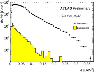
While elastic-scattering events are selected in the “golden” topology with two proton tracks in op- posite vertical detector positions on the left and right side, events in the “anti-golden” topology with two proton tracks in both upper or both lower detectors at the left and right side are pure background from accidental coincidences. After applying the event selection cuts, these events yield an estimate of background in the elastic sample with the golden topology. Furthermore, the anti-golden events can be used to calculate the form of the t-spectrum for background events by flipping the sign of the vertical coordinate on either side. As shown in Fig. 6, the background t-spectrum peaks strongly at small t and falls off steeply, distinguishably different from elastic events.
2] [GeV -t 0 0.05 0.1 0.15 0.2 0.25 0.3 0.35 ]-2 [GeVt/dNd
103
104
105
106
107
ATLAS Preliminary
b-1
µ
=7 TeV, 80 s
Data arm 1 Background
Figure 6: The counting rate dN/dt, before corrections, as a function of t in arm 1 compared to the background spectrum determined using anti-golden events. The form of the distribution is modified by acceptance effects (see Fig. 9).
Alternatively, the amount of background per arm is determined from the distribution of the horizontal vertex position at the interaction point, reconstructed using the beam optics transport Eq. (4). For elastic scattering, the vertex position peaks at small values of x, whereas for background the shape is much broader since halo background does not originate from the interaction point. Hence the fraction of background events can be determined from a fit to the measured distribution using templates.
The anti-golden method is used to estimate the background. Systematic uncertainties in the normal-
isation are taken from the difference between the anti-golden method and the vertex method, while the
background shape uncertainty is obtained from variations of the flipping procedure used to transform
the anti-golden events into elastic-like events. The expected numbers of background events are given in
Table 3 together with their uncertainties. The total uncertainty on the background is dominated by the
systematic uncertainty of 50–80%. Given the overall small background contamination of about 0.5%,
the large systematic uncertainty has only a small impact on the total cross-section determination.
Arm
++Arm
−−Numbers of background events 3329 1497
Statistical error
±58
±39
Systematic error
±1100
±1200
Table 3: Number of background events in each arm estimated with the anti-golden method and systematic uncertainties from the difference from the vertex method. The arm
++comprises all four upper detectors, the arm
−−all four lower detectors.
7.3 Event reconstruction e ffi ciency
Elastic-scattering events inside the acceptance region are expected to have a proton track in each of the four detectors of the corresponding spectrometer arm. However, in the case of interactions of the protons or halo particles with the stations or detectors, which result in too large fibre hit multiplicities, the track reconstruction described in Section 6.1 may fail. The rate of elastic-scattering events has to be corrected for losses due to such partly reconstructed events. This correction is defined as the event reconstruction efficiency.
A method based on a tag-and-probe approach is used to estimate the efficiency. Events are grouped into several reconstruction cases, for which different cuts and corrections are applied, to determine if an event is from elastically scattered protons, but was not fully reconstructed because of inefficiencies.
The reconstruction efficiency of elastic-scattering events is defined as
εrec =N
reco/(Nreco +N
fail), where N
recois the number of fully reconstructed elastic-scattering events, which have at least one recon- structed track in each of the four detectors of an spectrometer arm, and N
failis the number of not fully reconstructed elastic-scattering events, which have reconstructed tracks in fewer than four detectors. It does not include the efficiency of other selection cuts, which is discussed in Sec. 8, but is separate from any acceptance effects. Events of both classes need to have an elastic-scattering trigger signal and need to be inside the acceptance region, i.e. they have to fulfil the event selection criteria for elastic-scattering events. The efficiency is determined separately for the two spectrometer arms. Based on the number of detectors with at least one reconstructed track the events are grouped into six reconstruction cases 4/4, 3/4, 2/4, 1+1/4, 1/4 and 0/4. Here the digit in front of the slash indicates the number of detectors with at least one reconstructed track. In the 2/4 case both detectors with tracks are on one side of the interaction point and in the 1+1/4 case they are on different sides. With this definition one can write
εrec =
N
4/4N
4/4+N
3/4+N
2/4+N
1+1/4+N
1/4+N
0/4,
(15)
where N
k/4is the number of events with k detectors with at least one reconstructed track in a spectrometer arm.
Elastic-scattering events are selected for the various cases based on the event selection criteria de-
scribed in Section 7.1. The proton with reconstructed tracks on one side of the interaction point is used
as a tag and the one on the other side as a probe. Both tag and probe have to pass the event selection to be
counted as an elastic-scattering event and to be classified as one of the reconstruction cases. Depending
on the case only a sub-set of the event selection cuts can be used, because just a limited number of detec-
tors with reconstructed tracks is available. For example it is not possible to apply left-right acollinearity
cuts on 2/4 events, because tracks are only reconstructed on one side of the interaction point. To disen-
tangle the efficiency from acceptance, an additional cut on the minimum total fibre hit multiplicity (sum
of all fibre hits in the 20 layers of a detector; maximum is 1280 hits) in all detectors without any recon-
structed track is applied. This way, events where tracks could not be reconstructed due to too few fibre
hits are excluded from the efficiency calculation and only handled by the acceptance, which is discussed in Sec. 8.
6 8 10 12 14 16 18 20 22
Events / 0.2 mm
0 5 10 15 20 25 30 35
103
×
ATLAS Preliminary b-1 µ = 7 TeV, 80 s
2/4, A3, data 2011 3/4, A3, data 2011 4/4, A3, data 2011
[mm]
y
6 8 10 12 14 16 18 20 22
Ratio
0.5 1 1.5 2
Figure 7: Distribution of the vertical track po- sition at the detector surface for detector A3 of the 2/4 case (
•) where no track was recon- structed in A6 and A8, the 3/4 case (
◦) where no track was reconstructed in A8 and of the 4/4 case (
N). The distributions are normalized to the number of events of the distribution of the 4/4 case. The bottom panel displays ratios be- tween k/4 and 4/4 with statistical uncertainties.
2] [GeV t - 0 0.05 0.1 0.15 0.2 0.25 0.3 0.35
recε
0.88 0.9 0.92 0.94 0.96 0.98
1 ATLAS Preliminary
b-1
µ = 7 TeV, 80 s
Arm 1, data 2011 Linear fit to arm 1 Arm 2, data 2011 Linear fit to arm 2
Figure 8: Partial event reconstruction efficiency ˆ
εrecas a function of
−t for elastic arms 1 (
•) and 2 (
◦).
The solid line is a linear fit to arm 1 and the dashed one to arm 2.
With events from the 3/4 case it is possible to apply most of the event selection criteria and re- construct t well with the subtraction method. The position distribution of reconstructed tracks in 3/4 events agrees very well with that from 4/4 events, as shown in Fig. 7 for the vertical coordinate. Be- cause of this good agreement and the ability to reconstruct t, a partial event reconstruction efficiency
ˆ
εrec
(t)
=N
4/4(t)/[N
4/4(t)
+N
3/4(t)] as a function of t can be constructed, as shown in Fig. 8. Linear fits, applied to the partial efficiencies of each spectrometer arm, yield small residual slopes consistent with zero within uncertainties. This confirms that the efficiency
εrecin Eq. (15) is independent of t, as is expected from the uniform material distribution in the detector volume.
Two complications arise when counting 2/4 events. First, the vertical position distributions of the two detectors with reconstructed tracks do not agree with that from 4/4 events. As shown in Fig. 7 for A3, peaks appear at both edges of the distribution. These peaks are caused by events where protons hit the beam screen or thin Roman Pot window on one side of the interaction point and tracks are therefore only reconstructed on the other side. Since these events would be excluded by acceptance cuts, they are removed from the efficiency calculation. This is done by extrapolating the vertical position distribution from the central region without the peaks to the full region using the shape of the distribution from 4/4 events.
The second complication arises from single-diffraction background, which has a similar event topol-
ogy to the 2/4 events. This background is reduced by elastic-scattering trigger conditions, but an ir-
reducible component remains. Therefore, the fraction of elastic-scattering events is determined with a
fit, which uses two templates to fit the horizontal position distributions. Templates for elastic-scattering
events and a combination of single diffraction and other backgrounds are both determined from data. For
the elastic-scattering template events are selected as described in Sec. 7.1. Events for the background
template are selected based on various trigger signals that enhance the background and reduce the elastic- scattering contribution. The fit yields an elastic-scattering fraction in the range of r
el=0.88 to r
el=0.96 depending on the detector.
Because about 95% of N
failconsists of 3/4 and 2/4 events, the other cases play only a minor role.
Nevertheless, they are considered and included in the calculation. For cases 1+1/4 and 1/4 an additional event selection cut on the horizontal position distribution is applied to enhance the contribution from elastic scattering and suppress background. Edge peaks are present in the
y-position distributions of1/4 events and the extrapolation procedure, described above, is also applied. In the 0/4 case no track is reconstructed in any detector and the event selection criteria cannot be applied. Therefore, the number of 0/4 events is estimated from the probability to get a 2/4 event, which is determined from the ratio of the number of 2/4 to 4/4 events. The contribution to the reconstruction efficiency of this estimated number of 0/4 events is only about 1%.
The systematic uncertainties on the reconstruction efficiency are determined by varying the event selection cuts. Additional uncertainties arise from the choice of the central extrapolation region in
yfor 2/4 and 1/4 events and from the fraction fit. The uncertainties on the fraction fit are also determined by cut variation and an additional uncertainty is attributed to the choice of the background template.
The event reconstruction efficiencies in arm 1 and arm 2 are determined to be
εrec,1 =0.8974
±0.0004 (stat.)
±0.0061 (syst.) and
εrec,2 =0.8800
±0.0005 (stat.)
±0.0092 (syst.) respectively. The efficiency in arm 1 is slightly larger than in arm 2, due to differences in the detector configurations.
In arm 1 the trigger plates are positioned after the scintillating tracking fibres and in arm 2 they are
positioned in front of them. This leads to a higher shower probability and a lower efficiency in arm 2.
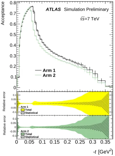
8 Acceptance and unfolding
The acceptance is defined as the ratio of events passing all geometrical and fiducial acceptance cuts defined in Section 7.1 to all generated events and is calculated as a function of t. The calculation is carried out with PYTHIA8 as elastic scattering event generator and MadX for beam transport based on the effective optics (see Section 9.2). The acceptance curve is shown in Fig. 9 for both arms. The shape
0 0.05 0.1 0.15 0.2 0.25 0.3 0.35
Acceptance
0 0.1 0.2 0.3 0.4 0.5 0.6 0.7 0.8
Arm 1 Arm 2
ATLAS Simulation Preliminary
=7 TeV s
0 0.05 0.1 0.15 0.2 0.25 0.3 0.35
Relative error
-0.1 -0.05 0 0.05 0.1
Arm 1 Total Statistical
2
] [GeV -t 0 0.05 0.1 0.15 0.2 0.25 0.3 0.35
Relative error -0.1-0.05
0 0.05 0.1
Arm 2 Total Statistical
Figure 9: The acceptance as function of the true value of t for both arms with total uncertainties being shown as error bars. The lower panels show relative total and statistical uncertainties.
of the acceptance curve can be understood from the contributions of the vertical and horizontal scattering
angles to t,
−t
=((θ
⋆x)
2+(θ
⋆y)
2)p
2. The smallest accessible value of t is obtained at the detector edge and
set by the vertical distance of the detector from the beam. Close to the edge, the acceptance is small as a
fraction of events is lost due to beam divergence, i.e. events being inside of the acceptance on one side
but outside at the other side. At small t up to
−t
∼0.07 GeV
2vertical and horizontal scattering angles
contribute about equally to a given value of t. Larger t-values imply larger vertical scattering angles and
larger values of
y, and with increasingythe fraction of events lost in the gap between the main detectors
decreases. The maximum acceptance is reached for events occurring at the largest values of
yclose to
the cut for the beam screen. Beyond that point the acceptance decreases steadily because only events at
larger values of x can contribute and the large-t values are dominated by the horizontal scattering angle
component. This explains also the difference between the two arms, which is dominated by the difference
between the respective beam-screen cuts.
The measured t-spectrum is affected by detector resolution and beam smearing effects, including angular divergence, vertex smearing and energy smearing. These effects are visible in the t-resolution and the purity of the t-spectrum. The purity is defined as the ratio of the number of generated and reconstructed events in a particular bin to the number of all events reconstructed in that bin. The purity is about 60% for the subtraction method, and is about a factor of two worse for the local angle method.
The limited t-resolution induces migration effects between bins that reduce the purity. Figure 10 shows the t-resolution for different t-reconstruction methods.
2] [GeV -t 0.05 0.1 0.15 0.2 0.25 0.3 0.35 [%]t)/rect-t(
5 10 15 20 25 30
35 ATLAS Simulation Preliminary
=7 TeV s
Subtraction method Local angle method Lattice method infinite det. resolution