Study of the spin of the new boson with up to 25 fb −1 of ATLAS data

A TLAS-CONF-2013-040 16 April 2013

ATLAS NOTE

ATLAS-CONF-2013-040

April 16, 2013

Study of the spin of the new boson with up to 25 fb ⁻¹ of ATLAS data

The ATLAS Collaboration

Abstract

This note presents a combined study of the spin of the Higgs boson candidate with a mass around 126 GeV which was observed in proton-proton collision data collected at the LHC with the ATLAS detector. Spin studies in the H → γγ, H → WW

→ `ν`ν and H → ZZ

→ 4` decays are combined to discriminate between the Standard Model assignment of J

= 0

and a specific model of J

= 2

. The dataset corresponds to an integrated luminosity of 20.7 fb

collected at a centre-of-mass energy of √

s = 8 TeV. For the H → ZZ

→ 4` decay mode an additional dataset corresponding to an integrated luminosity of 4.8 fb

collected at

√ s = 7 TeV is added. The data strongly favour the J

= 0

hypothesis. The specific J

= 2

hypothesis is excluded with a confidence level above 99.9%, independently of the assumed contributions of gluon fusion and quark-antiquark annihilation processes in the production of the spin-2 particle.

c

Copyright 2013 CERN for the benefit of the ATLAS Collaboration.

Reproduction of this article or parts of it is allowed as specified in the CC-BY-3.0 license.

1 Introduction

With the discovery of a new boson [1, 2] in the search for the Standard Model Higgs boson [3, 4, 5], the ATLAS and CMS experiments at the Large Hadron Collider (LHC) have reached an important milestone.

The observed production modes and decay rates of the new boson are compatible with those predicted for the Higgs boson of the Standard Model [6]. As a further important step towards understanding whether this particle is associated to the mechanism of the electroweak symmetry breaking and the mass generation of elementary particles, the Standard Model assignment of its quantum numbers has to be tested. In the Standard Model, the Higgs boson is a CP-even, spin-0 particle (J

= 0

). The Landau- Yang theorem forbids the direct decay of a spin-1 particle into a pair of photons [7, 8]. The spin-1 hypothesis is therefore strongly disfavoured by the observation of the H → γγ decay [1, 2].

The ATLAS collaboration has presented three independent studies of the spin of the new resonance.

The separation between the Standard Model J

= 0

and alternative hypotheses was studied in the bosonic decay channels H → γγ [9], H → WW

→ `ν`ν [10] and H → ZZ

→ 4` [11]. The full 2012 dataset collected at √

s = 8 TeV, corresponding to an integrated luminosity of about 21 fb

, is used for all three analyses. For the analysis of the H → ZZ

→ 4` channel, an additional dataset corresponding to an integrated luminosity of 4.8 fb

collected at √

s = 7 TeV is added. The observed final states are assumed to be produced in the decay of a single particle with a mass of 125.5 GeV [12]. The spin information is extracted from kinematic observables constructed from the final state particles in each of the channels considered.

In this note a combination of the spin studies performed in the three decay channels is presented.

The focus is discrimination between the Standard Model assignment of J

= 0

and a specific J

= 2

graviton-inspired model with minimal couplings to Standard Model particles. Since a spin-2 particle can be produced via both the gluon fusion process (gg) and the quark-antiquark annihilation (q q) process, ¯ the studies are generalized and admixtures of q q ¯ production between 0 and 100% are considered.

The note is organised as follows: in Section 2 details of the spin-2 models considered and of the Monte Carlo (MC) generators used in the analyses are presented. In Section 3 the analyses in the H → γγ, H → WW

→ `ν`ν and H → ZZ

→ 4` decay channels, as presented in Refs. [9, 10, 11], are briefly summarised. The statistical procedure employed for the combination of the individual results and the treatment of systematic uncertainties are discussed in Sections 4 and 5, respectively. Finally, in Section 6 the results of the statistical combination of individual channels are presented.

2 The spin-2 model and Monte Carlo samples

Given the large number of possible spin-2 models, a specific model from Ref. [13] was chosen. In this Reference, a spin-2 graviton-inspired model with minimal couplings to the Standard Model particles is defined via a choice of boson (g

= g

= 1 in Eq. 5 from Ref. [13]) and fermion couplings (ρ

= 1 in Eq. 10 from Ref. [13]). This choice of couplings implies that the production of the spin-2 particle is dominated by the gluon fusion process with a contribution, at leading order in QCD, of about 4% from quark-antiquark annihilation. Since the experimental observables are sensitive to the production mech- anisms the studies were performed by rescaling the production mechanisms in order to obtain fractions

f

of q q ¯ annihilation ranging from 0% to 100% in steps of 25%.

The production and decay of a spin-2 resonance is simulated using the JHU leading order generator

[13], version 2.02, interfaced to PYTHIA8 [14] for parton showering and hadronisation. The coupling

constants to bosons and fermions in JHU are defined as described above. In addition, the parameter

related to the scale of new physics (Λ) is set to 1 TeV. It should be noted, however, that the exact

choice of this parameter is irrelevant since the signal strengths in the individual channels are treated as

independent nuisance parameters. The JHU generator is also used to produce the Standard Model Higgs

boson signal in the gluon fusion process for the H → ZZ

→ 4` analysis. The angular distributions of final state particles were cross-checked using the POWHEG [15, 16] MC generator.

In the H → γγ and H → WW

→ `ν`ν analyses, the Standard Model Higgs boson signals pro- duced through the gluon fusion and vector boson fusion processes are generated at next-to-leading order by POWHEG, interfaced to PYTHIA8 for parton showering, hadronization and decays. Higgs boson production in association with a vector boson or a top-quark pair is simulated with PYTHIA8.

The samples are simulated with a mass of 125 GeV, whereas in the present analysis the mass value of 125.5 GeV is used, as determined from a combination of measurements in the H → γγ and H → ZZ

→ 4` channels [12]. In the H → γγ channel the small mass difference is taken into account by rescaling the transverse energies of the photons in the MC simulation by 0.4%. The impact of an equivalent rescaling of the lepton momenta in the H → WW

→ `ν`ν and H → ZZ

→ 4` analyses is found to be negligible and is not applied.

The transverse momentum (p

) distribution of the spin-0 signal generated with JHU + PYTHIA8 is re-weighted to agree with the resummed calculation from the HqT2 program [17]. The same set of weights is applied to the spin-2 signal produced via gluon fusion. This procedure emulates higher order QCD corrections under the assumption that they are identical for the spin-0 and the spin-2 particles.

A systematic uncertainty, taken as the full magnitude of this correction, is assumed. For the H → WW

→ `ν`ν decay channel it was demonstrated that the distributions of the sensitive observables are largely independent of the transverse momentum of the underlying resonance. The corresponding systematic uncertainties are thus neglected. For the p

distribution of the spin-2 particle produced via quark-antiquark annihilation no re-weighting is applied.

All samples are passed through a full MC simulation of the ATLAS detector [18] based on GEANT4 [19].

The simulation incorporates a model of the event pile-up conditions in the data, including both the e ff ects of multiple pp collisions in the same bunch crossing (“in-time” pile-up) and in nearby bunch crossings (“out-of-time” pile-up).

3 Individual channels

Detailed descriptions of the H → γγ, H → WW

→ `ν`ν and H → ZZ

→ 4` analyses are given in Refs. [9, 10, 11]; respectively. Only a brief review of each analysis is given below.

3.1 H → γγ

The diphoton decay channel is sensitive to the spin of the new boson through the measurement of the angular distribution of the photons in the resonance rest frame. Spin information can be extracted from the distribution of the absolute value of the cosine of the polar angle θ

of the photons with respect to the z-axis of the Collins-Soper (CS) frame [20] (noted | cos θ

| hereafter). This choice minimises the e ff ects from initial state radiation and results in better descriminating power than other options such as the beam axis or boost direction of the produced particle.

Apart from | cos θ

|, the separation between signal and background events (dominated by non-resonant

diphoton production after the event selection) makes use of the diphoton invariant mass (m

). The analy-

sis strategy consists of three steps. The first one is the selection of a pure sample of diphoton candidates,

as described in Ref. [9]. The next step is the modelling of the background distribution of | cos θ

| in

the signal region (122 GeV < m

< 130 GeV) using the invariant mass sidebands in data (defined by

105 GeV < m

< 122 GeV and 130 GeV < m

< 160 GeV). Finally, the two hypotheses are compared

via maximum likelihood fits. These fits are performed simultaneously in the sidebands – using only the

invariant mass distribution – and in the signal region, where the likelihood function is a product of the

one-dimensional probability density functions (pdfs) of | cos θ

| and m

, described below.

The invariant mass signal shape is expected to be dominated by detector effects since the signal intrinsic width is assumed to be very narrow in both the spin–0 and spin–2 hypotheses. Therefore, the same pdf is used to model both. The function chosen is the sum of a Crystal-Ball component accounting for about 95% of the signal events and a wide Gaussian component to describe outlying events. The invariant mass model of background events is a fifth degree polynomial, with coe ffi cients determined by a fit to the data.

The | cos θ

| distributions of both possible signals are obtained from MC. The spin-0 signal yields per

| cos θ

| bin are corrected for interference e ff ects with the non-resonant diphoton background gg → γγ [21].

The full size of the correction is taken as a systematic uncertainty, being sizeable only in the two highest bins of | cos θ

|. No interference between the spin-2 particle and the diphoton continuum background is assumed.

The modelling of the | cos θ

| distribution of background events in the signal region is the key as- pect of the analysis. The event selection uses cuts on the ratio of the photon transverse momentum to the invariant mass (p

/m

) in order to minimise the correlation between m

and | cos θ

|. Studies using the mass sidebands in data and high statistics MC samples of background events simulated by SHERPA [22] show that the residual correlations are typically below the percent level, reaching a few percent at | cos θ

| > 0.8. Therefore, the | cos θ

| pdf associated with background events in the signal region is assumed to be equal with that of the sidebands. Systematic uncertainties on the background model are uncorrelated across the bins of | cos θ

| and amount to about 1% (2–3%) at | cos θ

| < 0.8 (| cos θ

| > 0.8). The dominant component comes from the limited number of events in the sidebands in data, with an additional component arising from the residual correlation between the discriminant variables estimated with MC.

The largest separation between the two spin hypotheses in the two-photon decay channel occurs when the spin-2 particle is produced purely by gluon fusion. With increasing fractions of q q ¯ production, the | cos θ

| pdfs of the spin-0 and spin-2 signals become similar.

3.2 H → WW

→ `ν`ν

The analysis of the spin in the H → WW

→ `ν`ν channel is restricted to events containing two leptons of di ff erent flavour (one electron and one muon) and no observed jets with p

> 25 GeV and

|η| < 4.5. The jet p

threshold is increased to 30 GeV in the forward region 2.5 < |η| < 4.5 to reduce the influence of jets produced by pile-up. The leading lepton, corresponding to the triggering object, is required to have p

> 25 GeV and the sub-leading lepton p

> 15 GeV.

The major sources of backgrounds after the dilepton selection are: Z/γ

, di-boson and top quark (t¯ t and single top) production. W bosons produced in association with hadronic jets can be a large source of background if a jet is misidentified as a lepton. The requirement of two high- p

, isolated leptons significantly reduces the background contributions from fake leptons. Multijet and Z/γ

events are suppressed by requiring relative missing transverse energy

E

above 20 GeV.

Further lepton topological cuts are then applied to optimize the sensitivity for both J

= 0

and J

= 2

signals, namely the dilepton invariant mass m

< 80 GeV, the transverse momentum of the dilepton system p

> 20 GeV and the azimuthal angular di ff erence between leptons ∆ φ

< 2.8 radians.

These cuts significantly reduce the WW continuum and Z/γ

backgrounds.

Due to the presence of two neutrinos in the event, a full reconstruction of the various decay angles is not possible and instead a boosted decision tree (BDT) technique [23] is used to separate the spin hypotheses. Two separate BDT classifiers are developed: one classifier is trained to distinguish the J

= 0

signal from the sum of all backgrounds while the second classifier separates the J

= 2

sample

1E^miss_T,rel ≡E^miss_T ·sin∆φ, where∆φis the azimuthal separation between the missing transverse energyE^miss_T and the nearest reconstructed object (lepton or jet withpT>25 GeV) or ^π₂radians, whichever is smaller.

from the sum of all backgrounds. The training of each decision tree is performed using the following final state observables: m

, p

, ∆ φ

and m

, the transverse mass formed by the dilepton system and the missing transverse energy. The resulting two-dimensional distribution of both classifiers is then used in binned likelihood fits to test the compatibility with the presence of a J

= 0

or J

= 2

particle in the data. The analysis, including the retraining of the second classifier with the J

= 2

sample as signal, is repeated for each of the five values of f

.

The BDT makes use of the correlations between the input variables and relies on a good description of the input variables themselves as well as their correlations. Those have been studied in detail and found to be well described by simulation [10]. In addition, dedicated studies have been performed to verify that a BDT with the chosen four input variables is able to reliably separate the main backgrounds in a background enriched region and that the response is well modelled.

Two different categories of systematic uncertainties are considered: experimental or detector sources, such as jet energy scale or lepton identification efficiency, and theoretical sources such as the estimation of the e ff ect of higher-order contributions through variations of the QCD scale in the MC simulation.

Monte Carlo samples with systematically varied parameters were analysed using the BDT discriminant.

Both the overall normalization and shape distortions were incorporated as nuisance parameters in the likelihood.

The WW background in the signal region (SR) is evaluated through extrapolation from a control re- gion (CR) using simulation. The theoretical uncertainties on the extrapolation parameter α = N

/N

, the ratio of the number of events passing the signal region selection to the number passing the control region selection, are evaluated according to the prescription of Ref. [24]. Another important uncer- tainty arises from the shape modelling of the irreducible WW continuum background. To estimate this uncertainty, the shape di ff erence between the prediction from POWHEG + PYTHIA and the one from MC@NLO [25] + HERWIG [26] is assigned as a systematic uncertainty.

In this channel the discrimination between the J

= 0

and J

= 2

states rises rapidly with the fraction of q q ¯ production.

3.3 H → ZZ

→ 4`

The H → ZZ

→ 4` channel benefits from the presence of several spin-dependent observables and from the full reconstruction of the final state. The corresponding observables are the masses of the two Z bosons and five production and decay angles: θ

, Φ

, Φ, θ

and θ

. The masses of the intermediate Z bosons are calculated from the reconstructed 4-vectors of the final state leptons. Following the notation adopted in Ref. [11], these Z-bosons are denoted hereafter as Z

and Z

, where the index 1 is assigned to the Z boson whose observed mass is closest to the nominal PDG value. Their respective masses are defined as m

and m

. The full definition of the production and decay angles as well as the description of their variation for di ff erent spin and parity values can be found in Ref. [11]:

• θ

(θ

) is the angle between the negative final state lepton and the direction of flight of Z

(Z

) in the Z rest frame.

• Φ is the angle between the decay planes of the four final state leptons expressed in the four lepton rest frame.

• Φ

is the angle between the decay plane of the leading lepton pair and a plane defined by the vector of the Z

in the four lepton rest frame and the positive direction of the parton axis.

• θ

is the production angle of the Z

defined in the four lepton rest frame.

In contrast with the other channels, the spin studies in the H → ZZ

→ 4` decay do not require

the application of additional cuts. The observables sensitive to the spin and parity of the resonance are

reconstructed directly after the inclusive event selection described in Ref. [11]. The candidate events are selected in the region of reconstructed four lepton masses: 115 GeV < m

< 130 GeV. The irreducible ZZ background is estimated from the MC simulation. The reducible t¯ t, Zb b ¯ and Z + jets backgrounds are estimated from corresponding control regions in data.

The reconstructed observables are used to create multivariate discriminants trained to separate pairs of spin and parity states. Boosted decision trees, trained on simulated events after the full reconstruction and event selection, are used. Dedicated discriminants are created for the separation between the spin-2 hypotheses with given fractions of q q ¯ production contributions and the J

= 0

hypothesis.

The rejection power against the spin-2 model depends very weakly on f

. This is explained by the small role played in the separation by the production angles cos θ

, Φ, Φ

compared to the other observ- ables. The di ff erences in production angles induced by the nature of spin-2 production are expected to be small [13, 27]. The main contribution to the separation comes from the mass of the off-shell Z boson m

and from the decay angle cos θ

. Due to the similarity of the distributions of kinematic observables for both hypotheses, the separation between J

= 0

and J

= 2

is weak in the H → ZZ

→ 4` channel, compared to the other decay modes. A small dependence of the expected separation on the production contribution was, however, observed.

4 Statistical procedure and individual results

The statistical treatment in the combination follows the methodology used by the individual analyses [9, 10, 11]. A likelihood function L(, θ) with one parameter of interest is constructed as a product of conditional probabilities over the bins of the final discriminant in each channel (Eq. 1). The parameter of interest is defined as the fraction of J

= 0

signal, such that = 1 gives the Standard Model hypothesis, while = 0 represents the J

= 2

hypothesis. No a priori knowledge of the production cross sections or decay branching ratios is assumed. The number of signal events in each channel is a nuisance parameter in the likelihood:

L(, θ) =

Nbins

Y

i

P(N

| · S

(θ) + (1 − )S

(θ) + B

(θ)) ×

Nsys

Y

j

A( ˜ θ

|θ

) , (1) where θ represents all nuisance parameters. The likelihood function is a product of Poisson distributions P corresponding to the observation of N

events in each bin i, given the models of the spin-0 and spin-2 signals and the backgrounds (S

(θ), S

(θ) and B

(θ), respectively). Some of the nuisance parameters are constrained by auxiliary measurements through the functions A(˜ θ|θ).

The test statistic q used to distinguish between the two signal hypotheses is based on a ratio of likelihoods:

q = log L( = 1, θ ˆˆ

) L( = 0, θ ˆˆ

)

, (2)

where ˆˆ θ is the maximum likelihood estimator, evaluated under the J

= 0

or J

= 2

hypothesis.

The distributions of the test statistic for each of the two hypotheses are obtained using MC pseudo- experiments. The mean number of signal and background events in the pseudo-experiments is obtained from maximum likelihood fits to the data. In the fits of each pseudo-experiment, these and all other nuisance parameters are profiled.

The distributions of q are used in the estimation of the corresponding p

values p

( J

= 0

) and

p

( J

= 2

). The p

values are not, strictly speaking, probabilities of a given measurement being at least

as discrepant as the observation. Instead, they are associated to the expected and observed rejections of a

given hypothesis and are computed, respectively, by integrating the distribution of the tested hypothesis up to the median of the alternative hypothesis or the observed value. When the tested hypothesis corre- sponds to the true one, the observation is expected to be close to the median, corresponding to a p

-value around 50%; any deviation (either towards 0% or 100%) is a sign of a disagreement between the data and the tested hypothesis.

The exclusion of the spin-2 hypothesis in favour of the Standard Model J

= 0

hypothesis is evaluated in terms of the corresponding CL

( J

= 2

), defined as:

CL

(J

= 2

) = p

( J

= 2

)

1 − p

( J

= 0

) . (3)

4.1 Individual results

The expected and observed rejections of the J

= 0

and J

= 2

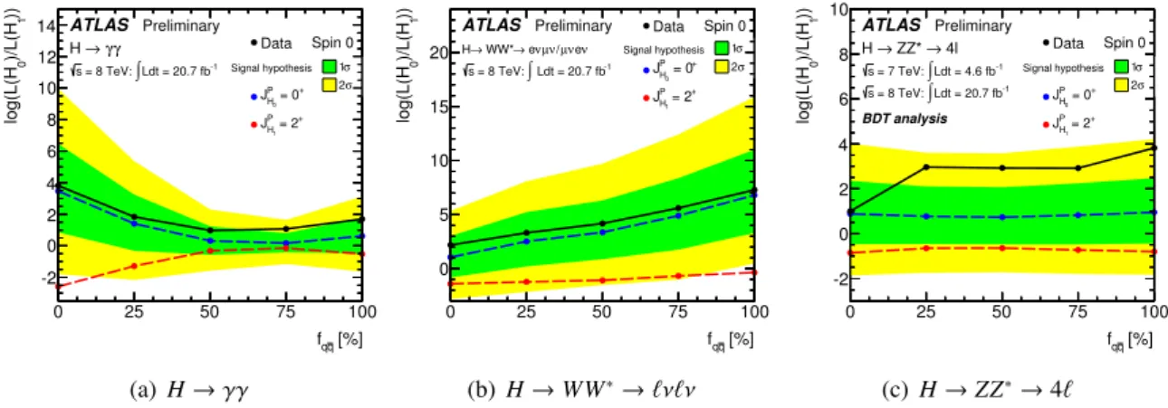
hypotheses in the three decay channels are summarised in Table 1, for all values of the fraction of q q ¯ production of the spin-2 particle considered. Figure 1 shows the values of the test statistic as a function of f

for all three channels. The blue and red dashed lines indicate the median values of the sampling distributions for pseudo-experiments generated under the spin-0 and spin-2 hypotheses, respectively.

For all three channels, the results are in good agreement with the spin-0 hypothesis. The results from the H → γγ channel exclude a spin-2 particle produced via gluon fusion at 99% CL

. As discussed in Section 3, the separation between the two spin hypotheses in this channel decreases with increasing f

. For the H → WW

→ `ν`ν decay channel, the results are in good agreement with the J

= 0

hypothesis. The J

= 2

hypothesis is excluded with a CL

confidence level up to 99% . Contrary to the H → γγ decay channel, the H → WW

→ `ν`ν analysis makes use of several final state observables.

As shown in Ref. [27], the angular distributions of a decay of a spin-2 particle into two massive bosons are much more complex than in the γγ case and di ff erent helicity states contribute. This explains the increase in the expected sensitivity with increasing f

in the H → WW

→ `ν`ν analysis.

As mentioned above, almost no dependence of the J

= 0

and J

= 2

separation on the spin-2 production mechanism is expected for the H → ZZ

→ 4` decay channel with the available dataset. The differences in the distributions of observables sensitive to the spin-2 production mechanism are too small.

A worse separation might be expected than in the H → WW

→ `ν`ν decay [27]. A separation above one standard deviation is expected for all tested values of f

. The data prefer the J

= 0

hypothesis.

For f

≥ 25% the observation is above the expected median for J

= 0

though still compatible within two standard deviations. This e ff ect is attributed to a fluctuation observed in the data.

As expected in the discussion presented above, the channels considered are complementary. The H → γγ channel provides the best expected sensitivity in the low f

region, while the separation is considerably reduced for f

≥ 50%. The H → WW

→ `ν`ν channel shows a moderate expected sensitivity at f

= 0% which grows rapidly for larger values of f

. Finally, the H → ZZ

→ 4` channel exhibits a small but stable expected sensitivity over the full range of f

.

5 Systematic uncertainties

The sources of systematic uncertainties accounted for in the analyses of the individual channels are listed in Refs. [9, 10, 11]. In the combination, the correlations among the common sources of the systematic uncertainties across channels are taken into account. These sources include the following contributions:

• Systematic uncertainties on electron and muon identification and reconstruction efficiencies, as

well as on their energy and momentum resolution are common to both the H → WW

→ `ν`ν and

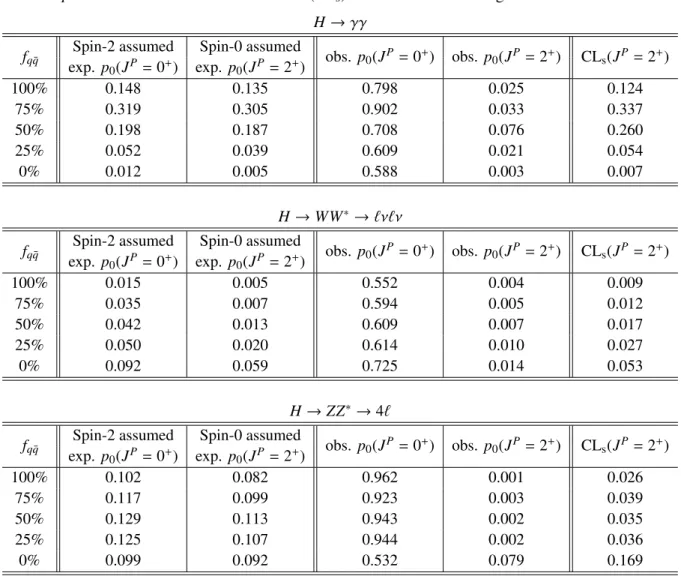
Table 1: Summary of results for the various fractions f

of the q q ¯ production of the spin-2 particle for the H → γγ (top), H → WW

→ `ν`ν (middle), and H → ZZ

→ 4` (bottom) decay channels.

The expected p

values for rejecting the J

= 0

and J

= 2

hypotheses (assuming the alternative hypothesis is true) are shown in the second and third columns. The fourth and fifth columns show the observed p0 values while the confidence levels (CL

) defined in the text are given in the last column.

H → γγ f

Spin-2 assumed Spin-0 assumed

obs. p

(J

= 0

) obs. p

(J

= 2

) CL

(J

= 2

) exp. p

(J

= 0

) exp. p

(J

= 2

)

100% 0.148 0.135 0.798 0.025 0.124

75% 0.319 0.305 0.902 0.033 0.337

50% 0.198 0.187 0.708 0.076 0.260

25% 0.052 0.039 0.609 0.021 0.054

0% 0.012 0.005 0.588 0.003 0.007

H → WW

→ `ν`ν f

Spin-2 assumed Spin-0 assumed

obs. p

(J

= 0

) obs. p

(J

= 2

) CL

(J

= 2

) exp. p

(J

= 0

) exp. p

(J

= 2

)

100% 0.015 0.005 0.552 0.004 0.009

75% 0.035 0.007 0.594 0.005 0.012

50% 0.042 0.013 0.609 0.007 0.017

25% 0.050 0.020 0.614 0.010 0.027

0% 0.092 0.059 0.725 0.014 0.053

H → ZZ

→ 4`

f

Spin-2 assumed Spin-0 assumed

obs. p

(J

= 0

) obs. p

(J

= 2

) CL

(J

= 2

) exp. p

(J

= 0

) exp. p

(J

= 2

)

100% 0.102 0.082 0.962 0.001 0.026

75% 0.117 0.099 0.923 0.003 0.039

50% 0.129 0.113 0.943 0.002 0.035

25% 0.125 0.107 0.944 0.002 0.036

0% 0.099 0.092 0.532 0.079 0.169

q [%]

fq

0 25 50 75 100

))1)/L(H0log(L(H

-2 0 2 4 6 8 10 12

14 ATLAS Preliminary γ

γ

→ H

Ldt = 20.7 fb-1

∫

= 8 TeV:

s

Data

Signal hypothesis

= 0+ H0

JP

= 2+ H1

JP

Spin 0 σ 1

σ 2

(a)H→γγ

q [%]

fq

0 25 50 75 100

))1)/L(H0log(L(H

0 5 10 15 20

ATLAS Preliminary ν νe µ ν/ µ ν

→ e WW*

→ H

= 8 TeV:

s ∫ Ldt = 20.7 fb^-1 Data

Signal hypothesis = 0+ H0

JP

= 2+ H1

JP

Spin 0 σ 1

σ 2

(b) H→WW^∗→`ν`ν

q [%]

fq

0 25 50 75 100

))1)/L(H0log(L(H

-2 0 2 4 6 8

10 ATLAS Preliminary

→ 4l

→ ZZ*

H

Ldt = 4.6 fb-1

∫

= 7 TeV:

s

Ldt = 20.7 fb-1

∫

= 8 TeV:

s

Data

Signal hypothesis

= 0+ H0

JP

= 2+ H1

JP

Spin 0 σ 1

σ 2 BDT analysis

(c) H→ZZ^∗→4`

Figure 1: Observed values of the test statistic (black solid line) as a function of the fraction of q q ¯ produc- tion of the spin-2 state f

for the H → γγ (a), H → WW

→ `ν`ν (b) and H → ZZ

→ 4` (c) channels.

The blue and red dashed lines indicate the positions of the median expected values of the sampling dis- tributions for the spin-0 and spin-2 signals, respectively, obtained from pseudo-experiments. The green and yellow bands correspond, respectively, to one and two standard deviations around the spin-0 median curve.

H → ZZ

→ 4` channels.

• Systematic uncertainties on the energy scale of electromagnetic objects (electrons and photons) affect all three decay channels. The associated nuisance parameters are correlated across the chan- nels.

• The systematic uncertainty on the measured luminosity is correlated among the H → WW

→

`ν`ν and H → ZZ

→ 4` channels. This uncertainty does not a ff ect the H → γγ channel, for which the background normalisation is extracted directly from fits to the data.

The common systematic uncertainty resulting from the method employed to determine the luminosity in the 2011 and 2012 datasets is not correlated among the channels. The corresponding effect is expected to be very small. It has also been verified that the results are nearly insensitive to variations of the Higgs boson mass within the measured accuracy of about ± 0.6 GeV [12].

6 Results of the combination

Table 2 shows the expected and observed p

values for both the J

= 0

and J

= 2

hypotheses for the combination of the H → γγ, H → WW

→ `ν`ν and H → ZZ

→ 4` channels. The results are shown as a function of the q q ¯ spin-2 production fraction. The compatibility of each spin hypothesis with the data is shown in Fig. 2. The test statistic calculated on data is compared to the corresponding expectations obtained from pseudo-experiments, as a function of f

. The number of pseudo-experiments performed to determine the distributions of the test statistics amount to 100k for the J

= 0

and 1 million for the J

= 2

hypothesis.

The data are in good agreement with the Standard Model J

= 0

hypothesis. The observed values in Fig. 2(a) are, however, found to be above the J

= 0

median values. This effect can be attributed to the aforementioned statistical fluctuation in the data of the H → ZZ

→ 4` decay channel.

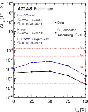
Figure 3 shows the comparison of the expected and observed CL

(J

= 2

) as a function of f

.

The expected exclusion of the spin-2 hypothesis shows only a weak dependence on f

, due to the com-

plementary sensitivities of the channels to the different production mechanisms of the spin-2 resonance,

Table 2: Expected and observed p

values for the J

= 0

and J

= 2

hypotheses as a function of the fraction f

of the q q ¯ spin-2 production mechanism. The values are calculated for the combination of the H → γγ, H → WW

→ `ν`ν and H → ZZ

→ 4` final states. The CL

values defined in the text are also presented.

f

Spin-2 assumed Spin-0 assumed

obs. p

(J

= 0

) obs. p

(J

= 2

) CL

(J

= 2

) exp. p

(J

= 0

) exp. p

(J

= 2

)

100% 3.4 · 10

9.4 · 10

0.82 0.4 · 10

0.2 · 10

75% 1.0 · 10

1.1 · 10

0.82 3.7 · 10

2.1 · 10

50% 1.5 · 10

3.5 · 10

0.85 9.1 · 10

6.0 · 10

25% 6.8 · 10

2.4 · 10

0.81 1.0 · 10

5.3 · 10

0% 1.6 · 10

6.1 · 10

0.65 1.4 · 10

4.0 · 10

q [%]

fq

0 25 50 75 100

)) 1)/L(H 0log(L(H

-10 0 10 20 30

40 ATLAS Preliminary

→ 4l ZZ*

→ H

Ldt = 4.6 fb-1

∫ = 7 TeV:

s

Ldt = 20.7 fb-1

∫ = 8 TeV:

s γ γ

→ H

Ldt = 20.7 fb-1

∫ = 8 TeV:

s

ν νe µ ν/ µ ν

→ e WW*

→ H

Ldt = 20.7 fb-1

∫ = 8 TeV:

s

Data Signal hypothesis

= 0+ H0

JP

= 2+ H1

JP

Spin 0

σ 1 σ 2

(a)

q [%]

fq

0 25 50 75 100

)) 1)/L(H 0log(L(H

-10 0 10 20 30

40 ATLAS Preliminary

→ 4l ZZ*

→ H

Ldt = 4.6 fb-1

∫ = 7 TeV:

s

Ldt = 20.7 fb-1

∫ = 8 TeV:

s γ γ

→ H

Ldt = 20.7 fb-1

∫ = 8 TeV:

s

ν νe µ ν/ µ ν

→ e WW*

→ H

Ldt = 20.7 fb-1

∫ = 8 TeV:

s

Data Signal hypothesis

= 0+ H0

JP

= 2+ H1

JP

Spin 2

σ 1 σ 2

(b)

Figure 2: Expected and observed ratio of profiled likelihoods for the combination of channels as a

function of the fraction of the q q ¯ spin-2 production mechanism. The green and yellow bands represent,

respectively, the one and two standard deviation bands for the J

= 0

(a) and for the J

= 2

(b)

hypotheses.

q

[%]

f

0 25 50 75 100

)

= 2

(J

CL

10

10

10

10

10

10

1 10 10

10

10

ATLAS

→ 4l ZZ*

→ H

Ldt = 4.6 fb-1

∫

= 7 TeV:

s

Ldt = 20.7 fb-1

∫

= 8 TeV:

s

γ γ

→ H

Ldt = 20.7 fb-1

∫

= 8 TeV:

s

ν νe µ ν/ µ ν

→ e WW*

→ H

Ldt = 20.7 fb-1

∫

= 8 TeV:

s

1σ 2σ

σ 3

4σ

Data

+)

P = 0 (assuming J

expected CLs

Figure 3: Expected (blue dashed line) and observed (black solid line) confidence level, CL

(J

= 2

), of the J

= 2

hypothesis as a function of the fraction of q q ¯ production of the spin-2 particle.

discussed in Section 3. The observed exclusion of the J

= 2

state in favour of the Standard Model J

= 0

hypothesis exceeds 99.9% CL for all values of f

.

7 Conclusion

A combined study of the spin of the Higgs boson candidate using the H → γγ, H → WW

→ `ν`ν and H → ZZ

→ 4` decay channels in the ATLAS experiment has been presented. The pp collision dataset corresponding to an integrated luminosity of 20.7 fb

collected at a centre-of-mass energy √

s = 8 TeV was used for all three decay channels. For the H → ZZ

→ 4` an additional dataset corresponding to an integrated luminosity of 4.8 fb

collected at 7 TeV was added.

The Standard Model assignment of J

= 0

is compared to a graviton-inspired J

= 2

model with minimal couplings to Standard Model particles. The data are in good agreement with the expected distributions of a J

= 0

particle while the graviton-inspired J

= 2

model, that is expected to be produced dominantly via the gluon fusion process, is excluded at more than 99.9% confidence level.

The most general spin-2 model involves a large number of parameters to fully describe the couplings of this resonance particle to the initial and final states relevant for the measurement of the spin. The analysis shown here does not address this general case. However, this study was extended to arbitrary admixtures of gluon fusion and q q ¯ production processes between 0 and 100%. In this extended study all J

= 2

production admixtures are excluded by the data at more than 99.9% confidence level.

References

[1] ATLAS Collaboration, Observation of a new particle in the search for the Standard Model Higgs

boson with the ATLAS detector at the LHC, Phys. Lett. B 716 (2012) 1, arXiv:1207.7214 [hep-ex].

[2] CMS Collaboration, Observation of a new boson at a mass of 125 GeV with the CMS experiment at the LHC, Phys. Lett. B 716 (2012) 30, arXiv:1207.7235 [hep-ex].

[3] F. Englert and R. Brout, Broken symmetry and the mass of gauge vector mesons, Phys. Rev. Lett.

13 (1964) 321.

[4] P. W. Higgs, Broken symmetries and the masses of gauge bosons, Phys. Rev. Lett. 13 (1964) 508.

[5] G. Guralnik, C. Hagen, and T. Kibble, Global conservation laws and massless particles, Phys.

Rev. Lett. 13 (1964) 585.

[6] ATLAS Collaboration, Combined coupling measurements of the Higgs-like boson with the ATLAS detector using up to 25 fb

of proton-proton collision data, ATLAS-CONF-2013-034 (2013).

[7] L. D. Landau, On the angular momentum of a two-photon system, Dokl. Akad. Nauk Ser. Fiz. 60 (1948) 207.

[8] C.-N. Yang, Selection Rules for the Dematerialization of a Particle Into Two Photons, Phys. Rev.

77 (1950) 242.

[9] ATLAS Collaboration, Study of the spin of the Higgs-like boson in the two photon decay channel using 20.7 fb

of pp collisions collected at √

s = 8 TeV with the ATLAS detector, ATLAS-CONF-2013-029 (2013).

[10] ATLAS Collaboration, Study of the spin properties of the Higgs-like boson in the H → WW

→ eνµν channel with 21 fb

of √

s = 8 TeV data collected with the ATLAS detector, ATLAS-CONF-2013-031 (2013).

[11] ATLAS Collaboration, Measurements of the properties of the Higgs-like boson in the four lepton decay channel with the ATLAS detector using 25 fb

of proton-proton collision data,

ATLAS-CONF-2013-013 (2013).

[12] ATLAS Collaboration, Combined measurements of the mass and signal strength of the Higgs-like boson with the ATLAS detector using up to 25 fb

of proton-proton collision data,

ATLAS-CONF-2013-014 (2013).

[13] Y. Gao et al., Spin determination of single-produced resonances at hadron colliders, Phys. Rev. D 81 (2010) 075022.

[14] T. Sjostrand, S. Mrenna, and P. Z. Skands, A Brief Introduction to PYTHIA 8.1, Comput. Phys.

Commun. 178 (2008) 852, arXiv:0710.3820 [hep-ph].

[15] S. Alioli, P. Nason, C. Oleari, and E. Re, NLO Higgs boson production via gluon fusion matched with shower in POWHEG, JHEP 0904 (2009) 002, arXiv:0812.0578 [hep-ph].

[16] P. Nason and C. Oleari, NLO Higgs boson production via vector-boson fusion matched with shower in POWHEG, JHEP 1002 (2010) 037, arXiv:0911.5299 [hep-ph].

[17] D. de Florian, G. Ferrera, M. Grazzini, and D. Tommasini, Transverse-momentum resummation:

Higgs boson production at the Tevatron and the LHC, JHEP 1111 (2011) 064, arXiv:1109.2109

[hep-ph].

[18] ATLAS Collaboration, The ATLAS simulation infrastructure, Eur. Phys. J. C 70 (2010) 823.

[19] GEANT4 Collaboration, S. Agostinelli et al., GEANT4: A simulation toolkit, Nucl. Instrum. Meth.

A 506 (2003) 250.

[20] J. C. Collins and D. E. Soper, Angular distribution of dileptons in high-energy hadron collisions, Phys. Rev. D 16 (1977).

[21] L. J. Dixon and M. S. Siu, Resonance continuum interference in the diphoton Higgs signal at the LHC, Phys. Rev. Lett. 90 (2003) 252001, arXiv:hep-ph/0302233 [hep-ph].

[22] T. Gleisberg et al., Event generation with SHERPA 1.1, JHEP 0902 (2009) 007, arXiv:0811.4622 [hep-ph].

[23] A. Hoecker et al., Toolkit for multivariate data analysis with ROOT, 2009.

[24] LHC Higgs Cross Section Working Group, S. Dittmaier, C. Mariotti, G. Passarino, and R. Tanaka (Eds.), Handbook of LHC Higgs Cross Sections: 2. Di ff erential Distributions, CERN-2012-002 (CERN, Geneva, 2012), arXiv:1201.3084 [hep-ph].

[25] S. Frixione and B. Webber, Matching NLO QCD computations and parton shower simulations, JHEP 0206 (2002) 029, hep-ph/0204244.

[26] G. Corcella et al., HERWIG 6: an event generator for hadron emission reactions with interfering gluons (including super-symmetric processes) , JHEP 0101 (2001) 010.

[27] S. Bolognesi et al., On the spin and parity of a single-produced resonance at the LHC, Phys. Rev.

D 86 (2012) 095031, arXiv:1208.4018 [hep-ph].

Appendix A

1)) )/L(H log(L(H0

-25 -20 -15 -10 -5 0 5 10 15 20 25

Arbitrary normalization

10-6

10-5

10-4

10-3

10-2

10-1

1 10 102

103 ^Data

Signal hypothesis = 0+ H0

JP q=0%

fq = 2+ H1

JP

ATLAS Preliminary

→ 4l ZZ*

→ H

Ldt = 4.6 fb-1

∫ = 7 TeV:

s

Ldt = 20.7 fb-1

∫ = 8 TeV:

s γ γ H →

Ldt = 20.7 fb-1

∫ = 8 TeV:

s

ν νe µ ν/ µ ν

→ e WW*

→ H

Ldt = 20.7 fb-1

∫ = 8 TeV:

s

(a)

1)) )/L(H log(L(H0

-25 -20 -15 -10 -5 0 5 10 15 20 25

Arbitrary normalization

10-6

10-5

10-4

10-3

10-2

10-1

1 10 102

103 ^Data

Signal hypothesis = 0+ H0

JP q=25%

fq = 2+ H1

JP

ATLAS Preliminary

→ 4l ZZ*

→ H

Ldt = 4.6 fb-1

∫ = 7 TeV:

s

Ldt = 20.7 fb-1

∫ = 8 TeV:

s γ γ H →

Ldt = 20.7 fb-1

∫ = 8 TeV:

s

ν νe µ ν/ µ ν

→ e WW*

→ H

Ldt = 20.7 fb-1

∫ = 8 TeV:

s

(b)

1)) )/L(H log(L(H0

-25 -20 -15 -10 -5 0 5 10 15 20 25

Arbitrary normalization

10-6

10-5

10-4

10-3

10-2

10-1

1 10 102

103 ^Data

Signal hypothesis = 0+ H0

JP q=50%

fq = 2+ H1

JP

ATLAS Preliminary

→ 4l ZZ*

H →

Ldt = 4.6 fb-1

∫ = 7 TeV:

s

Ldt = 20.7 fb-1

∫ = 8 TeV:

s γ γ H →

Ldt = 20.7 fb-1

∫ = 8 TeV:

s

ν νe µ ν/ µ ν

→ e WW*

→ H

Ldt = 20.7 fb-1

∫ = 8 TeV:

s

(c)

1)) )/L(H log(L(H0

-25 -20 -15 -10 -5 0 5 10 15 20 25

Arbitrary normalization

10-6

10-5

10-4

10-3

10-2

10-1

1 10 102

103 ^Data

Signal hypothesis = 0+ H0

JP q=75%

fq = 2+ H1

JP

ATLAS Preliminary

→ 4l ZZ*

H →

Ldt = 4.6 fb-1

∫ = 7 TeV:

s

Ldt = 20.7 fb-1

∫ = 8 TeV:

s γ γ H →

Ldt = 20.7 fb-1

∫ = 8 TeV:

s

ν νe µ ν/ µ ν

→ e WW*

→ H

Ldt = 20.7 fb-1

∫ = 8 TeV:

s

(d)

1)) )/L(H log(L(H0

-25 -20 -15 -10 -5 0 5 10 15 20 25

Arbitrary normalization

10-6

10-5

10-4

10-3

10-2

10-1

1 10 102

103 ^Data

Signal hypothesis = 0+ H0

JP

=100%

q fq = 2+ H1

JP

ATLAS Preliminary

→ 4l ZZ*

→ H

Ldt = 4.6 fb-1

∫ = 7 TeV:

s

Ldt = 20.7 fb-1

∫ = 8 TeV:

s γ γ

→

H ^{s = 8 TeV:} ∫Ldt = 20.7 fb-1

eν ν /µ ν µ eν WW* → H →

Ldt = 20.7 fb-1

∫ = 8 TeV:

s

(e)

Figure 4: Expected distributions of log(L(H

)/L(H

)) – the logarithm of the ratio of profiled likelihoods

under the spin-0 and spin-2 hypotheses – in the presence of spin-0 (blue distributions) or spin-2 (red

distributions) signals for various fractions of q q ¯ production of the spin-2 signal ( f

): (a) f

= 0%; (b)

f

= 25%; (c) f

= 50%; (d) f

= 75%; (e) f

= 100%. The observed values are indicated by

a vertical line. The coloured areas correspond to the integrals of the expected distributions up to the

observed values and are used to compute the p

values for the rejection of each hypothesis.

Table 3: Expected and observed p

values for J

= 0

and J

= 2

hypotheses as a function of the fraction f

of the q q ¯ spin-2 production mechanism. The values are calculated for the combination of the H → γγ, H → WW

→ `ν`ν and H → ZZ

→ 4` final states. The pseudo-experiments corresponding to the J

= 0

hypothesis are generated following the Standard Model predictions for the signal strength in each channel.

f

Spin-2 assumed Spin-0 assumed

obs. p

(J

= 0

) obs. p

(J

= 2

) CL

(J

= 2

) exp. p

(J

= 0

) exp. p

(J

= 2

)

100% 1.3 · 10

8.1 · 10

0.99 4.2 · 10

0.4 · 10

75% 2.3 · 10

1.3 · 10

0.96 3.7 · 10

1.0 · 10

50% 2.3 · 10

2.2 · 10

0.97 9.1 · 10

2.8 · 10

25% 1.0 · 10

2.1 · 10

0.97 1.0 · 10

4.1 · 10

0% 2.9 · 10

1.0 · 10

0.95 1.4 · 10

3.0 · 10