Measurement of the Higgs boson mass in the H √ → Z Z ∗ → 4` and H → γγ channels with s = 13 TeV p p collisions using the ATLAS

A TLAS-CONF-2017-046 10 July 2017

ATLAS CONF Note

ATLAS-CONF-2017-046

5th July 2017

Measurement of the Higgs boson mass in the H √ → Z Z ^∗ → 4` and H → γγ channels with s = 13 TeV p p collisions using the ATLAS

detector

The ATLAS Collaboration

The mass of the Higgs boson is measured in the H → Z Z

→ 4 ` and in the H → γγ decay channels with 36.1 fb

of proton-proton collision data from the Large Hadron Collider at a centre-of-mass energy of 13 TeV recorded by the ATLAS detector in 2015 and 2016. The measured value in the H → Z Z

→ 4 ` channel is

m

= 124 . 88 ± 0 . 37 GeV , while the measured value in the H → γγ channel is

m

= 125 . 11 ± 0 . 42 GeV .

The value of the Higgs boson mass obtained from a simultaneous fit to the invariant mass distributions in the two channels is

m

= 124 . 98 ± 0 . 28 GeV .

© 2017 CERN for the benefit of the ATLAS Collaboration.

1 Introduction

The observation of a new particle in the search for the Standard Model (SM) Higgs boson ( H ) by the ATLAS and CMS experiments [1, 2] with the LHC Run 1 data at center-of-mass energies of

√ s = 7 TeV and 8 TeV has been a major step towards understanding the mechanism of electroweak (EW) symmetry breaking [3–5]. The mass of the Higgs boson has been measured with a simultaneous fit to the ATLAS and CMS Run 1 data to be 125 . 09 ± 0 . 24 GeV [6], improving on the individual ATLAS [7] and CMS [8]

mass measurements. Further measurements of the spin, parity and couplings of the new particle have shown no significant deviations from the predictions for the SM Higgs boson [8–12]. With the increased center-of-mass energy and higher integrated luminosity of the Run 2 LHC data, the Higgs boson properties can be studied in further detail.

This note presents the measurement of the Higgs boson mass m

with 36.1 fb

of pp collision data recorded with the ATLAS detector at a center-of-mass energy of

√ s =13 TeV. The measurement of the mass of the Higgs boson is derived from a combined fit to the invariant mass spectra of the decay channels H → Z Z

→ 4 ` ( ` = e, µ ) and H → γγ , based on the current understanding of the reconstruction, identification, and calibration of muons, electrons, and photons in the ATLAS detector.

The note is organised as follows. In Section 2 a brief description of the ATLAS detector is given. Section 3 summarizes the data and simulation samples used in this study. A brief summary of the reconstruction, identification and calibration procedures is given in Section 4 for muons and in Section 5 for electrons and photons. The details of the Higgs boson mass measurements in the four leptons and diphoton channels are discussed in Section 6 and Section 7, respectively. The combined mass measurement in both channels is described in Section 8, and the conclusions are summarized in Section 9.

2 ATLAS detector

The ATLAS experiment [13] at the LHC is a multi-purpose particle detector with a forward-backward symmetric cylindrical geometry and nearly 4 π coverage in solid angle.1 It consists of an inner tracking de- tector surrounded by a thin superconducting solenoid providing a 2 T axial magnetic field, electromagnetic and hadron calorimeters, and a muon spectrometer.

The inner detector (ID) covers the pseudorapidity range |η | < 2 . 5. It consists of silicon pixel, silicon micro-strip, and transition radiation tracking detectors.

Lead/liquid-argon (LAr) sampling calorimeters provide electromagnetic (EM) energy measurements up to |η | = 3 . 2. For |η | < 2 . 5 the EM calorimeter is segmented into three longitudinal layers and has fine granularity in the transverse ( η – φ ) plane.

A hadron (steel/scintillator-tile) calorimeter covers the central pseudorapidity range ( |η | < 1 . 7). The end-cap and forward regions are instrumented with LAr calorimeters for both EM and hadronic energy measurements up to |η | = 4 . 9.

1

ATLAS uses a right-handed coordinate system with its origin at the nominal interaction point (IP) in the centre of the detector and the

-axis along the beam pipe. The

-axis points from the IP to the centre of the LHC ring, and the

-axis points upwards. Cylindrical coordinates

are used in the transverse plane,

being the azimuthal angle around the

The pseudorapidity is defined in terms of the polar angle

as

ln tan

2

. Angular distance is measured in units of

∆R≡

q(∆η)²+(∆φ)²

.

The muon spectrometer (MS) surrounds the calorimeters and is based on three large air-core toroidal superconducting magnets with eight coils each. The field integral of the toroids ranges between 2.0 and 6.0 T · m across most of the detector. The muon spectrometer includes a system of precision tracking chambers (for |η | < 2 . 7) and fast detectors for triggering (for |η | < 2 . 4).

A two-level trigger system is used for the on-line event selection. Events are selected using a first-level trigger implemented in custom electronics, which reduces the event rate below the design value of 100 kHz using a subset of the detector information. This is followed by a software-based trigger that exploits the full granularity and precision of the calorimeter and reduces the accepted event rate to 1 kHz on average by refining the first-level trigger selection.

3 Data and simulated samples

Data were collected at a pp centre-of-mass energy of 13 TeV during 2015 and 2016 using single–lepton, dilepton, trilepton and diphoton triggers. The identification, isolation and p

requirements applied to the single–lepton triggers were tighter than those used for the multi–lepton triggers. The combined efficiency of the lepton triggers for the H → Z Z

→ 4 ` events passing the offline selection is about 98%. Diphoton events were selected using a diphoton trigger with transverse energy ( E

) thresholds of 35 GeV and 25 GeV for the highest- E

(“leading”) and second-highest- E

(“subleading”) photon candidates. Both photon candidates were required to have an energy deposition in the calorimeter with a shape loosely consistent with the one expected from an electromagnetic shower initiated by a prompt photon not originating from a hadron decay. The diphoton trigger has an efficiency higher than 99% for H → γγ events passing the final event selection. After trigger and data-quality requirements, the integrated luminosity of the data sample is 36.1 fb

.

A Monte Carlo (MC) simulation is used in the analysis to model the detector response for signal and background processes. Except when noted, the generated events are passed through a Geant4 [14]

simulation of the response of the ATLAS detector [15] and reconstructed with the same algorithms as the data. Additional proton-proton interactions (pileup) are included in the simulation, matching the average number of interactions per bunch crossing to the value observed in the data.

For the signal, samples are simulated for several values of m

, separately for the two final states under study. For the H → Z Z

→ 4 ` decay, samples at m

equal to 120, 122, 124, 125, 126, 128 and 130 GeV are generated. For the H → γγ decay, samples at m

equal to 110, 122, 123, 124, 125, 126, 127, 130, 140 GeV are produced. Signal events are generated at all m

values for the four Higgs boson production modes with largest cross-section: gluon fusion (ggF), vector-boson fusion (VBF), and associated production with a vector boson V = W, Z (VH), for both q q ¯

→ V H and gg → Z H . For rarer processes, contributing to less than 2% of the total cross-section, only samples at m

= 125 GeV are used.

The POWHEG-BOX v2 Monte Carlo (MC) event generator [16–18] is used to simulate ggF [19], VBF [20]

and V H [21] processes, using the PDF4LHC15 NLO PDF set [22]. The ggF Higgs-boson production is ac-

curate to next-to-next-to-leading order (NNLO) in quantum chromodynamics (QCD), using the POWHEG

method for merging the next-to-leading order (NLO) Higgs-boson plus jet cross-section with the parton

shower, and the MiNLO method [23] to simultaneously achieve NLO accuracy for inclusive Higgs-boson

production. The VBF and V H samples are produced at NLO accuracy in QCD. For V H , the MiNLO

method is used to merge 0-jet and 1-jet events [24]. For Higgs-boson production in association with

a top quark ( t ) pair ( t¯ t H ), events are simulated at NLO with MadGraph5_aMC@NLO [25], using the NNPDF3.0 PDF set [26]. PYTHIA 8 [27] is used for the Higgs boson decay as well as for parton shower- ing, hadronisation, and multiple partonic interactions, using the AZNLO parameter set [28] for the ggF, VBF and V H production mechanisms, and the A14 parameter set [29] for the t¯ t H one.

The SM expectations are assumed for the Higgs boson production cross-section times branching ratio, in the various production modes and final states under study and at each value of m

, and used to normalise the simulated samples. The Higgs-boson production cross-sections and decay branching ratios, as well as their uncertainties, are taken from Refs. [30–33]. The cross-section for Higgs-boson production via ggF is computed at next-to-next-to-next-to-leading order (N3LO) accuracy in QCD and has next-to-leading order (NLO) electroweak (EW) corrections applied [34–47]. The cross-section for the VBF process is calculated with full NLO QCD and EW corrections [48–50], and approximate next-to-next-to-next-to-leading order (N3LO) QCD corrections are applied [51]. The cross-sections for the production of a Higgs boson in association with an electroweak boson, V H , are calculated at NNLO accuracy in QCD [52, 53] and NLO electro-weak (EW) radiative corrections [54] are applied. The cross-section for t t H ¯ production is calculated at NLO accuracy in QCD [55–58].

The Higgs-boson decay branching ratio to the four-lepton final state ( ` = e, µ ) for m

= 125.09 GeV is predicted to be ( 1 . 251 ± 0 . 027 ) × 10

[33, 59] in the SM using PROPHECY4F [60, 61], which includes the complete NLO QCD and EW corrections, and the interference effects between identical final-state fermions. Due to the latter, the expected branching ratios of the 4 e and 4 µ final states are about 10%

higher than the branching ratios to 2 e 2 µ and 2 µ 2 e final states. The branching ratio in the H → γγ channel is calculated with HDECAY [59] and PROPHECY4F and predicted to be ( 2 . 27 ± 0 . 07 ) × 10

at m

= 125 . 09 GeV [33].

The Z Z

continuum background from quark-antiquark annihilation is simulated with the Sherpa 2.2 [62–

64] event generator, using the NNPDF3.0 NNLO PDF set. NLO accuracy is achieved in the matrix element calculation for 0-jet and 1-jet final states and LO accuracy for 2- and 3-jet final states. The merging is performed with the Sherpa parton shower [65] using the MePs@NLO prescription [66]. NLO EW corrections are applied as a function of the invariant mass of the Z Z

system m

[67, 68]. The gluon-induced Z Z

production is modelled with gg2VV [69] at leading order in QCD. The k-factor accounting for missing higher order QCD effects in the calculation of the gg → Z Z

continuum is taken to be 1.7 ± 1.0 [70–74]. Sherpa 2.2 is also used to generate samples of the Z + jets background at NLO accuracy for 0-jet, 1-jet and 2-jet final states and LO accuracy for 3- and 4-jet final states. In this measurement, the Z + jets background is normalised using control samples from data. For comparisons with the simulation, the QCD NNLO fEWZ [75, 76] and NLO MCFM [77] cross-section calculations are used for inclusive Z boson and Z + b b ¯ production, respectively. Samples for the t t ¯ background are produced with POWHEG interfaced to PYTHIA 6 [78] for parton shower and hadronisation, to PHOTOS [79] for quantum electrodynamics (QED) radiative corrections, to Tauola [80, 81] for the simulation of τ lepton decays and to EvtGen for the simulation of b -hadron decays. For this sample, the Perugia 2012 parameter set [82] is used. The W Z background is modelled using POWHEG+PYTHIA 8 and the AZNLO parameter set. The triboson backgrounds Z Z Z , W Z Z , and W W Z with four or more leptons originating from the hard scatter are produced with Sherpa 2.1. MadGraph, interfaced to PYTHIA 8 with the A14 parameter set, is used to simulate the all-leptonic t¯ t + Z as well as the t¯ t + W process.

The main irreducible background for H → γγ is from continuum diphoton production. These events

are simulated with up to three additional partons in the final state using Sherpa 2.1, with the CT10

PDF [83] and the default parameter set for underlying event activity. V γγ event samples are produced

using Sherpa 2.1 with up to two additional partons in the final state. The very large sample size required

for the modelling of the γγ background processes is obtained through a fast parametric simulation of the ATLAS detector response [15].

4 Muon reconstruction and calibration

Muon track reconstruction is first performed independently in the ID and in the MS. Hit information from the individual sub-detectors is then used in a combined muon reconstruction, which is performed according to various algorithms based on the information provided by the ID, the MS and the calorimeters.

The muon reconstruction and identification performance is described in detail in Ref. [84].

Although the simulation accurately describes the ATLAS detector, additional corrections to the simulated momentum are needed in order to match the simulation to data precisely. The muon momentum resolution and momentum scale are parametrised as a power expansion in the muon p

, with each extracted term measured separately for the ID and MS, as a function of η and φ , from large samples of J/ψ → µ

µ

and Z → µ

µ

decays [84].

The momentum scale calibration constants account for the inaccurate measurement of the energy loss in the traversed material, for any deficiency in the description of the magnetic field integral, and for the inaccurate description of the dimension of the detector in the direction perpendicular to the magnetic field. The momentum resolution calibration constants account for local magnetic field inhomogeneities and multiple scattering as well as for intrinsic resolution effects and local radial distortions. The main sources of uncertainties on these calibration constants arise from non-Gaussian resolution tails, background modelling and alignment uncertainties studied using data taken without the toroidal magnetic field [84].

Such uncertainties are conservatively assumed to be fully correlated across η and φ . In the muon momentum range used for the m

measurement, the momentum scale is known to a precision of one to two per mille for central muons, and to a precision of two to five per mille for forward muons [84]. The resolution is known with a precision ranging from one to two percent for central muons and around ten percent for forward muons.

The data taken in 2016 were affected by significant local misalignments of the ID. These misalignments bias the muon track sagitta, leaving the track χ

invariant [85, 86]. The bias on the track sagitta, δ

(η, φ), is of the order of 1 TeV

depending on η and φ , and result in a charge-dependent bias of the reconstructed muon momentum. Since the sagitta bias affects positive and negative muons in opposite directions, for neutral objects the effect at first order of these biases is a worsening of the resolution and no impact on their average reconstructed mass. Denoting p

T

and p

T

the initial and corrected muon momentum respectively, the effect is parametrised as:

p

T

( µ) = p

T

( µ) 1 − q( µ) δ

(η, φ) p

T

( µ) (1)

where q is the muon charge. These biases are studied and corrected in data by comparing the local inhomogeneities of the charge dependent dimuon mass to the mass of well-known neutral resonances. An iterative correction on each muon momentum is derived by subtracting the bias of Eq. (1) at each iteration.

Starting from percent-level sagitta biases, the residual effect after correction is reduced to the per-mille

level at the scale of the Z -boson mass. The correction improves the resolution of the dimuon invariant

mass in Z -boson decays by 1% to 5%, depending on η and φ . The systematic uncertainty associated to

this correction is estimated for each muon using simulation. The total uncertainty varies as a function

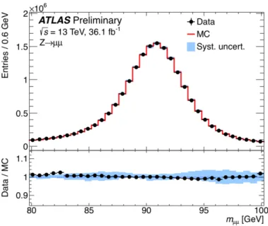
Figure 1: Inclusive dimuon invariant mass distribution of Z → µ

µ

candidate events. The upper panel shows the invariant mass distribution for data and for simulation. The points show the data after correction for local charge- dependent momentum biases. The continuous line corresponds to the simulation with the momentum corrections applied. The band represents the total systematic uncertainty on the momentum corrections. The lower panel shows the data to simulation ratio. No subtraction of the background (expected to be at the level of 0.5% and with a non-peaking distribution) is applied, and the simulation is normalised to the data.

of η , φ and p

, and is found to be about 20 MeV for the average momentum of muons from Z → µ

µ

decays.

The invariant mass distributions of dimuons from Z → µ

µ

decays in data and simulation after such corrections are compared in Figure 1. After corrections data and simulation agree to better than 3% for the description of the Z -boson decay lineshape.

5 Photon and electron reconstruction, identification and calibration

Photon and electron candidates are reconstructed from clusters of energy deposited in the electromagnetic calorimeter [87]. Clusters without a matching track or reconstructed conversion vertex in the inner detector are classified as unconverted photons. Those with a matching reconstructed conversion vertex or a matching track, consistent with originating from a photon conversion, are classified as converted photons. Clusters matched to a track consistent with originating from an electron produced in the beam interaction region are considered electron candidates.

The energy measurement for reconstructed electrons and photons is performed by summing the energies

measured in the EM calorimeter cells belonging to the candidate cluster. The energy is measured from a

cluster size of ∆ η × ∆ φ = 0 . 075 × 0 . 175 in the barrel region of the calorimeter and ∆ η × ∆ φ = 0 . 125 × 0 . 125

in the calorimeter endcaps. The calibration strategy for the energy measurement of electrons and photons

follows closely the one described in Ref. [88], with updates to reflect the 2015 and 2016 data taking conditions.

• Firstly, the cluster energy is corrected for energy loss in the inactive materials in front of the calorimeter, the fraction of energy deposited outside the area of the cluster in the η − φ plane and for the amount of energy deposited into the hadronic calorimeter. Further corrections are applied to account for the variation of the energy response as a function of the impact point in the calorimeter. The calibration coefficients used to apply these corrections are obtained from a detailed simulation of the detector response to electrons and photons, and are optimised with a boosted decision tree (BDT). The response is calibrated separately for electrons, converted and unconverted photon candidates.

• Secondly, the global calorimeter energy scale is determined in situ with a large sample of Z → e

e

events, and verified using J/ψ → e

e

and Z → `

`

γ events. The energy response in data and simulation is equalised by applying η -dependent correction factors to match the invariant mass distributions of Z → e

e

events. The energy scale correction factors are typically of the order of 1–2% with an uncertainty ranging from 0.01% to 0.1%. In this procedure, the simulated width of the reconstructed Z boson mass is matched to the one observed in data by adding in the simulation a contribution to the constant term of the electron energy resolution. This constant term varies between 0.7%–2% for |η | < 2 . 4 with an uncertainty of 0.1%–0.2%.

A comparison between the invariant mass distribution of selected Z → e

e

candidates in data and simulation after having applied the energy scale corrections to data and the resolution adjustment to the simulation is shown in Figure 2.

The main sources of systematic uncertainties in the calibration procedure discussed in Ref. [88] have been revisited. These sources include uncertainties in the relative calibration of the different gains used in the calorimeter readout, in the knowledge of the material in front of the calorimeter, in the intercalibration of the different calorimeter layers, in the modelling of the lateral shower shapes and in the reconstruction of photon conversions. The total calibration uncertainty for photons with E

around 60 GeV is 0.4% in the barrel and 0.8% in the endcap. In the case of electrons with E

around 40 (10) GeV the total uncertainty is 0.02% (0.5%) in the barrel and 0.1% (0.8%) in the endcap.

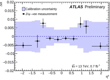
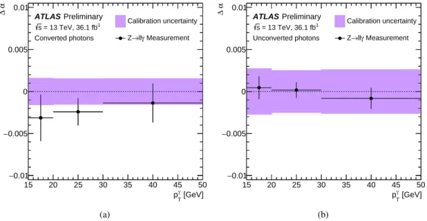
Residual electron response corrections, after applying the corrections extracted from the Z → e

e

samples, are computed independently on a sample of J/ψ → e

e

events and found to be compatible with zero within the uncertainties, as shown in Figure 3. A similar check is performed by computing residual corrections for photons in a sample of radiative Z boson decays and found to be compatible with zero within uncertainties, as shown in Figure 4.

Systematic uncertainties in the calorimeter energy resolution arise from uncertainties in the modelling of the sampling term and on the measurement of the constant term in Z boson decays, in the amount of material in front of the calorimeter, which affect electrons and photons differently, and in the modelling of the small contribution to the resolution from fluctuations in the pile-up from other proton-proton interactions in the same or neighbouring bunch crossings. The uncertainty on the calorimeter energy resolution is typically 10–20% for photons from Higgs boson decays, and varies from 5% to 10% for electrons in the E

range from 10 GeV to 45 GeV.

The photon identification is based primarily on shower shapes in the calorimeter. The two levels of

selection, loose and tight, are described in Ref. [89]. To further suppress the number of jets in the photon

candidate samples, two complementary isolation selection criteria are used, based on topological clusters

[MeV]

mee

Events / 0.5 GeV

0 200 400 600 800 1000 1200

103

×

Preliminary ATLAS

=13 TeV, 36.1 fb-1

s

→ee Z

Calibrated data Corrected MC Scale factor uncert.

[GeV]

mee

80 82 84 86 88 90 92 94 96 98 100

Data / MC

0.9 0.95 1 1.05 1.1

Figure 2: Inclusive dielectron invariant mass distribution from Z → e

e

decays in data compared to MC after applying the full calibration. No subtraction of the background (expected to be at the level of 0 . 5% and with a non-peaking m

distribution) is applied, and the simulation is normalised to data. The lower panel shows the data to simulation ratio, together with the total scale factor uncertainty.

−2 −1.5 −1 −0.5 0 0.5 1 1.5 2 ηe

−0.02 0.015

−

−0.01 0.005

− 0 0.005 0.01 0.015

α∆ 0.02 ATLAS Preliminary

= 13 TeV, 0.7 fb-1

s Calibration uncertainty

ee measurement

→ ψ J/

Figure 3: Energy calibration scale factors ∆α obtained from J/ψ → e

e

samples after having applied the Z -based

calibration, as a function of the electron pseudorapidity in the reference frame of the calorimeter. The error bars on

the data points represent the total uncertainty specific to the J/ψ → e

e

analysis and include both statistical and

systematic uncertainties. The band represents the calibration systematic uncertainty extrapolated from Z → e

e

events. The luminosity is the sum of the prescaled luminosities collected by the J/ψ triggers in 2015 and 2016. The

corresponding unprescaled luminosity is 36.1 fb

.

[GeV]

γ

pT

15 20 25 30 35 40 45 50

α∆

−0.01 0.005

− 0 0.005 0.01

Calibration uncertainty Measurement γ

→ll Z Preliminary ATLAS

= 13 TeV, 36.1 fb-1

s

Converted photons

(a)

[GeV]

γ

pT

15 20 25 30 35 40 45 50

α∆

−0.01 0.005

− 0 0.005 0.01

Calibration uncertainty Measurement γ

→ll Z Preliminary ATLAS

= 13 TeV, 36.1 fb-1

s

Unconverted photons

(b)

Figure 4: Energy calibration scale factors ∆α for (a) photons converted to e

e

and (b) unconverted photons, computed with a double ratio method using Z → eeγ and Z → µµγ events, after having applied the Z -based calibration, as a function of the photon transverse momentum. The error bars on the data points represent the total uncertainty specific to the Z → ``γ measurement and include both statistical and systematic uncertainties. The purple band represents the calibration systematic uncertainty extrapolated from Z → e

e

events.

of energy deposits in the calorimeter and on on reconstructed trucks in a direction close to that of the photon candidate, as described in Ref. [90].

Electrons are identified using a likelihood-based method combining information from the electromagnetic

calorimeter and the tracker. As in the case of photons, electrons are required to be isolated using both

calorimeter-based and track-based isolation variables. More details are given in Ref. [91].

6 Mass measurement in the H → Z Z ^∗ → 4` channel

6.1 Event selection and background estimation

Events are required to contain four isolated charged leptons ( ` = e, µ ) which fulfil certain kinematic conditions. The leptons are grouped into two pairs of oppositely charged leptons of the same flavour and that emerge from a common vertex. A more complete description of the event selection can be found elsewhere [92]. In comparison with the selection used in the Run 1 measurement, the p

threshold for the lowest- p

lepton in the quadruplet has been lowered from 6 to 5 GeV for muons and a 4 ` vertex cut has been added to counter-balance the increase of reducible background caused by this reduced p

threshold. The lepton pair with an invariant mass closest (second closest) to the Z boson pole mass in each quadruplet is referred to as the leading (subleading) dilepton pair. The selected events are split according to the flavour of the leading and subleading pairs; ordered according to the expected selection efficiency, they are 4 µ , 2 e 2 µ , 2 µ 2 e , 4 e . If more than four leptons are found in the event, only the quadruplet with the largest expected efficiency is kept. Finally, reconstructed photon candidates passing final-state radiation selections are combined with the lepton quadruplet, and a kinematic fit is performed to constrain the invariant mass of the leading lepton pair to the Z pole mass [7]. Using the corrected value of m

, events with 110 < m

< 135 GeV are used for the Higgs boson mass measurement.

The selected events have a small contribution from reducible background processes: Z +jets, t¯ t , and W Z production which are selected if at least one of the jets in the final states is misidentified as a prompt isolated electron or muon. Non-resonant Z Z

production with a final state topology similar to the H → Z Z

→ 4 ` signal is the main background contribution. This process, as well as a much smaller contribution from t¯ tV ( V = Z , W ) and triboson production, is modelled using simulation normalised to the SM prediction, as described in Section 3. The contribution of the reducible background to the signal region (SR) is obtained from data in control regions (CR) formed by inverting and/or relaxing selections with respect to the SR. The CRs are defined according to the flavour of the subleading dilepton ( µµ or ee ) and the selections are aimed at providing data samples enhanced in the corresponding backgrounds while minimising contamination from Z Z

and the signal. The contributions of each background source to the yield in each CR are disentangled with fits to the mass of the leading dilepton pair and are extrapolated to the signal region with transfer factors obtained from MC simulation. Details on the method can be found in Ref.[92], together with background estimates in the signal region, inclusive in m

. The background estimate for the mass measurement is obtained by scaling the inclusive estimate according to the fraction that corresponds in the m

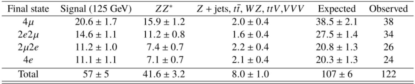
range that is fitted, estimated from both simulation and the data CR. The expected yields for a signal of 125 GeV and backgrounds are shown in Table 1 and are found to be in good agreement with the observed yields in all channels.

The Higgs boson is more centrally produced than the non-resonant Z Z

production and tends to have larger transverse momentum. The transverse momentum and pseudorapidity of the four-lepton system are therefore used together with a matrix-element-based kinematic discriminant D

[93] as inputs to a boosted decision tree (BDT) to discriminate the H → Z Z

→ 4 ` signal from the Z Z

→ 4 ` background.

D

is defined as ln(|M

|

/|M

|

) where M

denotes the matrix element for leading order

gluon fusion mediated H → Z Z

→ 4 ` production and M

the corresponding matrix element for

the q q ¯ → Z Z

continuum background calculated with MadGraph5 [25]. No cut on the value of the

BDT output is applied, but the events are categorised in four exclusive equal-size BDT bins in order

to better separate the signal from the background contribution in the m

fit. The separation of signal

Table 1: The number of events expected and observed for a signal under a m

=125 GeV hypothesis and the backgrounds considered in the analysis in each of the four-lepton final states in the range 110 < m

< 135 GeV.

All numbers are quoted with their total uncertainty.

Final state Signal (125 GeV) Z Z

Z + jets, t t ¯ , W Z , ttV , V V V Expected Observed 4 µ 20 . 6 ± 1 . 7 15 . 9 ± 1 . 2 2 . 0 ± 0 . 4 38 . 5 ± 2 . 1 38 2 e 2 µ 14 . 6 ± 1 . 1 11 . 2 ± 0 . 8 1 . 6 ± 0 . 4 27 . 5 ± 1 . 4 34 2 µ 2 e 11 . 2 ± 1 . 0 7 . 4 ± 0 . 7 2 . 2 ± 0 . 4 20 . 8 ± 1 . 3 26 4 e 11 . 1 ± 1 . 1 7 . 1 ± 0 . 7 2 . 1 ± 0 . 4 20 . 3 ± 1 . 3 24

Total 57 ± 5 41 . 6 ± 3 . 2 8 . 0 ± 1 . 0 107 ± 6 122

from background brought by the BDT output brings 6% improvement on m

resolution in the 4 ` decay channel.

The mass of the Higgs boson is determined from the position of the peak in the four-lepton invariant mass distribution around 125 GeV. This distribution is a superposition of a signal distribution S

, which is a function of the mass of the Higgs boson m

, and a background distribution B , which is independent of m

. The determination of the background distribution B is described above. The shape of the signal distribution depends on the four-lepton invariant mass resolution which varies event by event. This variation is taken into account by the so-called “per-event method” as described below.

6.2 Per-event method

The measured m

signal distribution is modelled as the convolution of the intrinsic Higgs boson lineshape, assumed to be a relativistic Breit-Wigner ( BW ) distribution with width equal to the SM value and mass m

free in the fit, with a four-lepton invariant mass response function F , which gives the probability of measuring a value m

4`

for a true invariant mass m

4`

: S

(m

4`

) =

∞

Z

0

F (m

4`

− m

4`

) · BW (m

4`

, m

) dm

4`

. (2)

The response function is derived using simulation from the lepton energy response functions which describe the probability of measuring a lepton energy E

given its true energy E

. The lepton energy response functions can be parametrised by a linear superposition of three normal distributions. The parameters of the normal distributions and their linear coefficients are different for electrons and muons, and they depend on both the lepton energy and the detector region in which the lepton energy is measured.

The parametrization as a sum of normal distributions was chosen because it is possible to express the four-lepton invariant mass response function as a convolution of 3

= 81 normal distributions, whose parameters can be computed from the parameters of the lepton energy response functions. Since the shape of the lepton energy response function depends on the lepton kinematics, their combination forming the four-lepton invariant mass response function varies from one event to another.

The procedure outlined above provides the four-lepton invariant mass response for the signal as a sum of

eighty-one normal distributions. In order to simplify the probability density function (pdf), the number of

normal distributions can be reduced, while minimising the loss of information, by following a procedure

which is also used in the Gaussian sum filter of the electron reconstruction software [94]. The similarity

of the eighty-one normal distributions is quantified by the Kullback-Leiber distance D

[95] defined for a pair of normal distributions labelled by a and b by:

D

=

σ

− σ

+ ( µ

− µ

)

σ

+ σ

σ

σ

. (3)

In the first step the pair of normal distributions with the smallest value of D

is replaced by a single normal distribution with the mean value, the standard deviation, and the weight set to the corresponding values of the sum of the two normal distributions. This replacement procedure is repeated until one has reached four normal distributions, which provides sufficient precision as determined from studies.

In principle, the same per-event approach used for the signal could be applied to derive the background pdf. However, as the background has a relatively flat distribution, there is no gain. So the per-event method is applied only to derive the signal pdf.

As the uncertainty on the mass measurement depends linearly on the resolution, the m

resolution is improved by constraining the mass of the leading lepton pair to the lineshape of the Z boson [7]. This allows about 15% improvement in the four-lepton mass resolution, and is the most significant improvement for this measurement. However, there is a drawback to the Z mass constraint in the fact that it introduces a correlation between the measured energies of the two leptons from the Z boson decay which cannot be analytically incorporated into the basic method. This is treated with an empirical approach. In a first step, the lepton energy response functions are determined after the Z mass constraint and the parameters of the four normal distributions which model the four-lepton invariant mass response functions are derived from these lepton energy response functions. In a second step, the parameters of the four normal distributions are rescaled by factors which have been extracted from simulation to reproduce the four-lepton invariant mass response.

Finally, the mass of the Higgs boson m

is determined by maximising the likelihood function:

L (m

) = Y

k=1

f S

m

4`

+ B

m

4`

g

as a function of m

where the index k denotes the k

event and N the number of selected events and B the pdf for the background. The expected statistical uncertainty on m

for a data sample of the size of the experimental set is of ± 0 . 34 GeV.

6.3 Validation of the per-event method with Z → 4` events

The per-event method was not only tested with simulated Higgs decays, but also with Z → 4 ` events reconstructed in simulation and in data. In this test, BW (m

4`

, m

) in Equation (2) is replaced by a relativistic Breit-Wigner distribution with a free pole mass m

and the natural width set to the width of the Z boson. B is used to allow for a tiny background from Z + jets events.

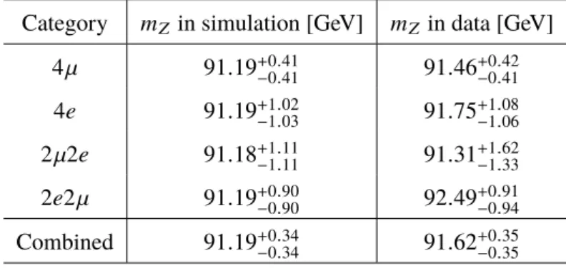
Table 2 summarises the measured value of the Z -boson mass in the different final state categories for simulation and data. The measured values agree with the world average of the Z -boson mass within less than one standard deviation in the simulation and within less than 1 . 3 standard deviations in data. The error estimates in data are found to be compatible with the errors expected from simulation.

Additional details and figures are discussed in Appendix A.

Table 2: Validation of the mass determination method with simulated and data Z → 4 ` events. The table summarises the values of the measured Z -boson mass by final state category and after the combination of the results from the individual final states.

Category m

in simulation [GeV] m

in data [GeV]

4 µ 91 . 19

91 . 46

4 e 91 . 19

91 . 75

2 µ 2 e 91 . 18

91 . 31

2 e 2 µ 91 . 19

92 . 49

Combined 91 . 19

91 . 62

0.35

6.4 Template method

An alternative signal model, used as a cross check in this analysis, is called the template method [6].

This method builds a template distribution for S

from simulation at different simulated masses, and interpolates these shapes to intermediate mass points. This provides a continuous distribution for S

. The simulation is used to compare the template method with the per-event method. While both the per- event and template methods are unbiased for a sufficiently large sample and when the lepton kinematics are well modelled by simulation, the m

values obtained by the template method are subject to resolution fluctuations for small samples. The performance of both methods has been studied with sets of pseudo- experiments for a small sample of events. The m

estimates of the template method are found to differ from the per-event method with a variance of about 0 . 16 GeV. The statistical uncertainty on m

obtained with the template method for a data sample of the size of the experimental data set and is about 1 . 4%

worse than that of the per-event method.

The per-event method is less model dependent since it constructs the m

signal distribution from the lepton response whereas the template method includes assumptions on, for example, the Higgs p

distribution included in the simulation. In addition, the per-event method has a small expected statistical uncertainty and is less sensitive to fluctuations in small-sized datasets. For these reasons the per-event method has been chosen as the baseline method for the mass determination in the H → Z Z

→ 4 ` channel.

6.5 Systematic uncertainties

As the Higgs boson mass is determined from a fit of an S + B distribution with a signal distribution

S depending on the lepton energy response functions, the measured Higgs boson mass depends on

the normalisation of the fit function, the lepton energy resolution, and the lepton energy scale. These

are included as nuisance parameters in the likelihood function, and constrained within uncertainties to

the estimates obtained from auxiliary data or simulation control samples by penalty terms multiplying

the likelihood. The systematic uncertainty in the measured mass is expected to be small compared

to the expected statistical uncertainty, and to be dominated by the lepton energy and momentum scale

uncertainties.

6.6 Results

The estimate of m

for the per-event and template methods is extracted with a simultaneous profile likelihood fit to the sixteen categories (one for each final state and for each BDT bin) of data. The observed total uncertainty in m

for the per-event method is of ± 0 . 37 GeV. For the template method it is found to be

GeV, larger by about 35 MeV than for the per-event method.

[GeV]

4l

m

110 115 120 125 130 135

Events / 2.5 GeV

0 10 20 30 40 50 60

ATLAS Preliminary

= 13 TeV, 36.1 fb-1

s

4l

*→ ZZ H→

Data Fit Background

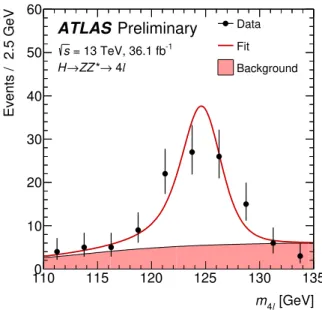
Figure 5: Invariant mass distribution of the data (points with error bars) shown together with the projection of the simultaneous fit result to H → Z Z

→ 4 ` candidates (continuous line). The background component of the fit is also shown (filled area). The signal pdf is evaluated per-event and averaged over the observed data.

The observed difference for the m

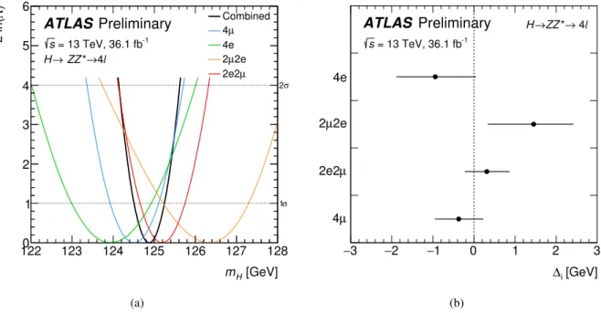
estimates of the two methods is found to be 0 . 16 GeV, which is compatible with the expected variance estimated with pseudo-experiments and corresponds to a one sided p-value of 0.19. Figure 5 shows the addition of the projections of the fits with the per-event method to the different categories compared to the combined 4 ` data. The fit is also performed independently for each decay channel fitting all BDT categories simultaneously; the resulting likelihood profile is compared to the combined fit in Figure 6 (a) and the projections of the fit results to the data for each decay channel are shown in Figure 7.

Here and in the following results, including those of the γγ decay channel and the combination of the two

final states, the statistical uncertainty on m

is determined by fixing all nuisance parameters to their best-

fit values, except for those that do not correspond to systematic uncertainties and are thus unconstrained

in the nominal fit ( i.e. , in the 4 ` final state, the signal production cross section). This approach yields

the lower bound on the statistical uncertainty, when the combination of different categories is performed

neglecting the different impact of the systematic uncertainties in each category. The total systematic

uncertainty is found by subtracting in quadrature the statistical uncertainty from the total uncertainty. The

systematic uncertainty due to each source is found by leaving free all the nuisance parameters except for

the unconstrained ones and for those corresponding to the source under study, repeating the fit, and then

subtracting in quadrature this reduced uncertainty obtained from the original total uncertainty.

With such procedure, the measured value of m

is found to be

m

= 124 . 88 ± 0 . 37 ( stat ) ± 0 . 05 ( syst ) GeV = 124 . 88 ± 0 . 37 GeV ,

as evaluated from the per-event method. The total uncertainty is in agreement with the expectation of

± 0 . 35 GeV and is dominated by the statistical component. The variance of the expected uncertainty was estimated to be 60 MeV. The total systematic uncertainty is 47 MeV, with the leading sources being the muon momentum scale (40 MeV), the electron energy scale (20 MeV), the background modelling (10 MeV) and the simulation statistics ( 8 MeV), as summarized in Table 3.

Table 3: Leading sources of systematic uncertainty on m

in the H → Z Z

→ 4 ` channel.

Systematic effect Uncertainty on m

[MeV]

Muon momentum scale 40

Electron energy scale 20

Background modelling 10

Simulation statistics 8

The combined measured value of m

is found to be compatible with the value measured independently for each channel with deviations ranging from about 0 . 6 σ for the 4 µ channel to about 1 . 3 σ for the 2 µ 2 e channel, as shown in Figure 6 (b).

[GeV]

mH

122 123 124 125 126 127 128

)Λ-2 ln(

0 1 2 3 4 5 6

1σ 2σ

ATLAS Preliminary

= 13 TeV, 36.1 fb-1

s

4l

*→

→ZZ H

Combined 4µ 4e

2e 2µ 2e2µ

(a)

[GeV]

∆i

3

− −2 −1 0 1 2 3

4µ 2e2µ 2e 2µ

4e

ATLAS Preliminary

= 13 TeV, 36.1 fb-1

s

4l

*→

→ZZ H

(b)

Figure 6: (a) Value of − 2 ln Λ as a function of m

for the combined fit to all H → Z Z

→ 4 ` categories. (b)

Observed differences between the combined m

value in the H → Z Z

→ 4 ` channel from the per-event method

and that of each final state obtained independently. Error bars correspond to the total uncertainties.

[GeV]

4l

m

110 115 120 125 130 135

Events / 2.5 GeV

0 5 10 15 20 25

ATLAS Preliminary

= 13 TeV, 36.1 fb-1

s

4µ

*→

→ZZ H

Data Fit Background

(a)

[GeV]

4l

m

110 115 120 125 130 135

Events / 2.5 GeV

0 5 10 15 20 25

ATLAS Preliminary

= 13 TeV, 36.1 fb-1

s

2e2µ

*→

→ZZ H

Data Fit Background

(b)

[GeV]

4l

m

110 115 120 125 130 135

Events / 2.5 GeV

0 5 10 15 20 25

ATLAS Preliminary

= 13 TeV, 36.1 fb-1

s

2e 2µ

*→

→ZZ H

Data Fit Background

(c)

[GeV]

4l

m

110 115 120 125 130 135

Events / 2.5 GeV

0 5 10 15 20 25

ATLAS Preliminary

= 13 TeV, 36.1 fb-1

s

4e

*→ ZZ H→

Data Fit Background

(d)

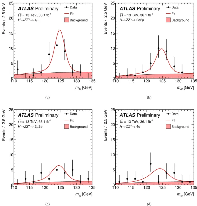
Figure 7: Invariant mass distribution of the data for each decay channel of H → Z Z

→ 4 ` (points with error bars)

shown together with the result of the simultaneous fit to all BDT categories for that channel projected to the data

(continuous line). The background component of the fit is also shown (filled area). The signal pdf is evaluated

per-event and averaged over the observed data.

7 Mass measurement in the H → γγ channel

The signal of the Higgs boson is observable as a narrow resonant peak in the diphoton invariant mass distribution m

above a large falling continuum background.

Events are selected and categorised as for the measurement of the total cross-section, simplified template cross-sections, and production mode signal strengths of the Higgs boson in the diphoton decay channel [90].

The categories have different mass resolution and purity; the overall signal-to-background ratio is a few percent. Compared to Ref. [90], a more complex signal model parametrisation as a function of m

is used as described below.

7.1 Event selection and categorisation

A first preselection is applied requiring at least two reconstructed photons with E

> 25 GeV and

|η | < 2 . 37, excluding the region 1 . 37 ≤ |η | ≤ 1 . 52 since the calorimeter granularity in the barrel–endcap transition region of the EM calorimeter is reduced, and the presence of significant additional inactive material upstream of the calorimeter affects the identification capabilities and energy resolution. Photons are required to pass loose identification criteria.

The two reconstructed photon candidates with the largest E

are considered and used to identify the diphoton primary vertex among all reconstructed vertices. Identifying the position of the primary vertex corresponding to the pp collision that produced the diphoton candidate is important to keep the contribution of the opening angle resolution to the diphoton mass resolution significantly smaller than the energy resolution contribution. In addition a correct identification of the tracks from the collision is also needed to avoid pile-up contributions to the track isolation. A neural network algorithm combines the information from the tracks and primary vertices, as well as the direction of the photons measured using the calorimeter and also the inner detector in the case of converted photons. The algorithm selects the correct diphoton vertex within 0.3 mm along the pp collision axis in 79% of simulated gluon-fusion events. For the other Higgs boson production modes this fraction ranges from 84% to 97%, increasing with jet activity or the presence of charged leptons. The leading and the subleading photons are required to have E

/m

> 0 . 35 and 0.25 respectively, and to pass the tight identification criteria and isolation criteria based on calorimeter and tracking information. Only events with 105 GeV ≤ m

≤ 160 GeV are kept.

For the events passing the selection discussed above, other objects are reconstructed and selected as jets,

b -jets, electrons, muons and missing transverse momentum. The details are reported in Ref. [90]. The

properties of the two selected photons and of the additional selected objects are used to categorise the

events in 31 mutually exclusive categories. The categories are optimised for the measurement of the

simplified template cross-sections [33, 96]. The most populated category, targeting gluon-gluon fusion

production without reconstructed jets, is split in two categories of events with very different energy

resolution: the first one (“ggH 0J CEN”) requires both photons to have |η | ≤ 0 . 95, while the second

one (“ggH 0J FWD”) retains the remaining events. To increase signal-to-background ratio, in the ttH

hadronic, VH hadronic and VBF categories, BDTs based on the kinematic properties of the diphoton and

jets in the event are used. Table 4 summarises the definition of the categories. It was observed that using a

categorisation as the one optimised for the previous mass measurement using Run 1 data [7] can improve

the total expected uncertainty only by 4%.

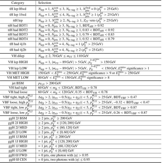
Table 4: Event selection defining each category. The category names denote the predominant production process or kinematic properties the category targets. Jets are required to have p

> 30 GeV unless otherwise noted. Jets are considered as forward (“fwd”) if they have |η | > 2 . 5. The categories are exclusive and criteria are applied in descending order of the shown categories. More details are provided in Ref. [90].

Category Selection tH lep 0fwd

= 1,

jets ≤

3,

1,

jets

= 0 (

T >

25 GeV) tH lep 1fwd

= 1,

jets ≤

4,

1,

jets ≥

1 (

T >

25 GeV) ttH lep

1,

jets ≥

2,

1,

veto (

T >

25 GeV) ttH had BDT1

= 0,

3,

1, BDT

0

92

ttH had BDT2

= 0,

3,

1, 0

83

BDT

0

92 ttH had BDT3

= 0,

3,

1, 0.79

BDT

0.83 ttH had BDT4

= 0,

3,

1, 0.52

BDT

0.79

tH had 4j1b

= 0,

jets

= 4,

= 1 (

T >

25 GeV) tH had 4j2b

= 0,

jets

= 4,

2 (

T >

25 GeV) VH dilep

2, 70 GeV

110 GeV

VH lep HIGH

1,

89 GeV

5 GeV,

T >

150 GeV VH lep LOW

1,

89 GeV

5 GeV,

T <

150 GeV,

T

significance

1 VH MET HIGH 150 GeV

T <

250 GeV,

T

significance

9 or

T >

250 GeV VH MET LOW 80 GeV

T <

150 GeV,

T

significance

8 jet BSM

200 GeV

VH had tight 60 GeV

120 GeV, BDT

0

78 VH had loose 60 GeV

120 GeV, 0

35

BDT

0

78

VBF tight, high

2,

0

5

5,

25 GeV, BDT

0

47 VBF loose, high

2,

0

5

5,

25 GeV,

0

32

BDT

0

47

VBF tight, low

2,

0

5

5,

25 GeV, BDT

0

87 VBF loose, low

2,

0

5

5,

25 GeV, 0

26

BDT

0

87

ggH 2J BSM

2 jets,

T ≥

200 GeV ggH 2J HIGH

2 jets,

T ∈

[120

200] GeV ggH 2J MED

2 jets,

T ∈

[60, 120] GeV ggH 2J LOW

2 jets,

T ∈

[0, 60] GeV ggH 1J BSM

1 jet,

T ≥

200 GeV ggH 1J HIGH

1 jet,

T ∈

[120

200] GeV ggH 1J MED

1 jet,

T ∈

[60

120] GeV ggH 1J LOW

1 jet,

T ∈

[0

60] GeV

ggH 0J FWD

0 jets, one photon with

0.95

ggH 0J CEN

0 jets, two photons with

0

95

7.2 Signal models

For each category the shape of the diphoton invariant mass distribution is modelled with a double-sided Crystal Ball function, i.e. a Gaussian function in the peak region with power-law functions in both tails.

Ignoring a normalisation factor, the distribution is described by the function:

f ( m

) =

 

 

 

 

 



 

 

 

 





e

if − α

≤ t ≤ α

e⁻¹2α2 low

1

Rlow(R_low−α_low−t)

nlow

if t < −α

e^−12αhigh2

1

Rhigh

(

)

if t > α

where t = (m

− µ

)/σ

, R

=

low

, and R

=

high

. µ

and σ

represent the position of the peak and the width of the Gaussian distribution, while α

, α

, n

and n

are parameters related to the tails.

The dependence of the parameters on the Higgs boson mass m

is fixed by fitting simultaneously all the simulated signal samples generated for different values of m

, weighting properly the production modes for the different cross-sections. To check the accuracy of the procedure a new model is generated ignoring one sample at m

and then it is fitted to the sample generated at m

. Using various values of m

the relative bias on the fitted Higgs boson mass is found to be less than 10

.

The resolution σ

at m

= 125 . 09 GeV is estimated as half of the smallest range containing 68% of the expected signal events and its value ranges between 1.42 and 2.14 GeV depending on the category, while for the inclusive case its value is 1.87 GeV. Figure 8 shows an example of the signal model for a category with excellent invariant mass resolution and for a category with poor resolution. Table 5 summarises the properties of the signal in each category.

The expected signal yield is parametrised as the product of integrated luminosity, production cross-section, diphoton branching ratio, acceptance and efficiency. The cross-section is parametrised as a function of m

separately for each production mode; similarly the branching ratio is parameterized as a function of m

; the product of acceptance and efficiency is evaluated separately for each production mode using only the samples with m

= 125 GeV and assumed to be constant. The cross-sections are fixed to the SM values multiplied by a signal modifier for each production mode: µ

, µ

, µ

and µ

.

7.3 Background models

In each category, the invariant mass distribution of the sum of all background processes is parameterized

with a continuous function. The parameters of these functions are fitted directly on data, as the number

of background events. The functional form used to describe the background in each category is chosen,

according to the procedure described in Ref. [90], as the one that minimises the fitted signal yield on

a sample of background only events. This background only sample is built from events selected from

control regions or from simulations depending on the background process. A minimum χ

probability

requirement for the fit of the background control sample with the chosen function is also required.

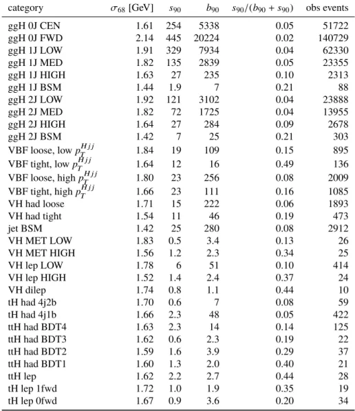
Table 5: Summary of the properties of the signal models, background models and observed number of events in data for each category. The numbers in the inclusive case are also reported in the last row of the table. Columns show the half-width σ

of the smallest m

interval containing 68% of the expected signal events, the number of fitted signal events in the smallest interval expected to contain 90% of the signal events ( s

), the number of background events in the smallest interval containing 90% of the signal model b

, the purity s

/(b

+ s

) in the same interval, and the total number of selected events in data in the range 105 GeV < m

< 160 GeV used for the fit.

category σ

[GeV] s

b

s

/(b

+ s

) obs events

ggH 0J CEN 1.61 254 5338 0.05 51722

ggH 0J FWD 2.14 445 20224 0.02 140729

ggH 1J LOW 1.91 329 7934 0.04 62330

ggH 1J MED 1.82 135 2839 0.05 23355

ggH 1J HIGH 1.63 27 235 0.10 2313

ggH 1J BSM 1.44 1.9 7 0.21 88

ggH 2J LOW 1.92 121 3102 0.04 23888

ggH 2J MED 1.82 72 1725 0.04 13955

ggH 2J HIGH 1.64 27 284 0.09 2678

ggH 2J BSM 1.42 7 25 0.21 303

VBF loose, low p

1.84 19 109 0.15 895

VBF tight, low p

1.64 12 16 0.49 136

VBF loose, high p

1.80 23 256 0.08 2009

VBF tight, high p

1.66 23 111 0.16 1085

VH had loose 1.71 15 222 0.06 1893

VH had tight 1.54 11 46 0.19 473

jet BSM 1.42 25 280 0.08 2912

VH MET LOW 1.83 0.5 3.4 0.13 26

VH MET HIGH 1.56 1.2 2.3 0.34 25

VH lep LOW 1.78 6 51 0.10 414

VH lep HIGH 1.52 1.4 2.4 0.37 24

VH dilep 1.74 0.8 1.1 0.44 10

tH had 4j2b 1.70 0.6 7 0.08 59

tH had 4j1b 1.66 2.3 48 0.05 422

ttH had BDT4 1.63 2.3 14 0.14 125

ttH had BDT3 1.62 0.6 2.3 0.19 22

ttH had BDT2 1.59 1.6 3.9 0.29 37

ttH had BDT1 1.60 1.3 2.0 0.40 21

ttH lep 1.62 2.2 2.7 0.44 28

tH lep 1fwd 1.72 1.0 1.9 0.35 19

tH lep 0fwd 1.67 0.9 3.6 0.20 34

[GeV]

γ

mγ

115 120 125 130 135 140

/ 0.5 GeVγγ1/N dN/dm

0 0.02 0.04 0.06 0.08 0.1 0.12 0.14 0.16

Simulation Preliminary ATLAS

= 13 TeV s = 125 GeV

, mH

γ γ

→ H

ggH 0J Cen MC Model ggH 0J Fwd

MC Model

Figure 8: Invariant mass distributions (circles) of simulated H → γγ events reconstructed in two categories with one of the best (“ggH 0J CEN”: open circles) and one of the worst (“ggH 0J FWD”: solid circles) experimental resolutions. The signal model derived from a fit of the simulated events is superimposed (solid lines).

An F -test is performed on data-sidebands to check whether functions with extra degrees of freedom describe the data significantly better. A test statistic is computed from the number of degrees of freedoms and χ

values of two binned fits to the data, with the nominal background model or with a model with an extra degree of freedom. The value of the test statistic obtained in the data is compared to the expected distribution obtained from pseudo data produced by assuming that the function with fewer degrees of freedom is the true underlying model. The simpler model is rejected in favor of the more complex one if the probability of finding larger values of the test statistic than in data is lower than 5%.

Usually this procedure selects simple exponential distributions for the categories with less events while power-law functions or exponential functions of a second-order polynomial are used for the others.

7.4 Systematic uncertainties

In order of importance, the sources of systematic uncertainty in the measured Higgs boson mass in the diphoton channel are the following: uncertainties in the photon energy scale (PES), in the chosen background model, in the primary vertex position, and other, smaller uncertainties. They are described in more detail in Ref. [90].

The dominant sources of uncertainty in the measured value of m

are the uncertainties in the PES. Each effect described in Section 5 is propagated to the diphoton invariant mass separately for each category.

The total effect on the mass ranges from ± 0 . 22% in the ggH 0J CEN category to ± 0 . 39% in the jet BSM category. All the PES effects are considered as fully correlated across categories.

The uncertainty due to the background modelling is evaluated following the procedure described in

Ref. [7]. First a test sample representative of the data background is built by combining simulation and

control regions in data. Then the expected signal contribution as predicted by the signal model is added

to the test sample. Finally the bias on the estimated Higgs boson mass from a signal plus background

fit to the test sample with respect to the injected mass is considered as a systematic uncertainty due to