Boosted Higgs (→ b b) Boson Identification with the ATLAS ¯ Detector at √

(1)

ATLAS-CONF-2016-039 08August2016

ATLAS NOTE

ATLAS-CONF-2016-039

30th July 2016

Boosted Higgs (→ b b) Boson Identification with the ATLAS ¯ Detector at √

s = 13 TeV

The ATLAS Collaboration

Abstract

This document summarises the baseline boosted Higgs boson identification strategy for Run 2 data collected by the ATLAS detector at a centre-of-mass energy of √

s = 13 TeV, as updated for the analysis of the 2015 and 2016 data. BoostedH → bb¯ decays are reconstructed from jets found with the anti-kt R = 1.0 jet algorithm, that are trimmed using a subjet radius ofRsubjet = 0.2 and a minimum transverse momentum fraction of fcut = 5%.

To tag Higgs bosons, requirements are applied on the following quantities:b-jets identified usingR=0.2 track jets matched to the large-Rcalorimeter jet, the trimmed jet mass and the trimmed jet energy correlation ratioD^(β₂⁼¹⁾. The Higgs boson tagging efficiency and corresponding multi-jet and hadronic top background rejections in simulated events are presented.

Several benchmark tagging selections are defined based on specific signal efficiency targets.

Systematic uncertainties on the Higgs tagging efficiency and background rejection resulting from uncertainties on theb-tagging efficiency, mass and D^(β₂⁼¹⁾variables are provided. In addition, theb-tagging performance at smallb-quark angular separations and the modelling of the jet properties, including jet substructure variables, are tested in a highp_Tg→bb¯ rich sample of large-Rjets fromppcollisions at √

s=13 TeV recorded in 2015.

c

2016 CERN for the benefit of the ATLAS Collaboration.

Reproduction of this article or parts of it is allowed as specified in the CC-BY-4.0 license.

(2)

1 Introduction

The increase of the LHC centre-of-mass energy to 13 TeV, and the increase in luminosity, greatly extends the sensitivity of the ATLAS experiment [1] to heavy new particles. In a significant number of new physics scenarios [2–4], these heavy new particles may have decay chains including the recently discovered Higgs boson [5,6]. The large mass of these resonances implies that a large momentum will be imparted to the Higgs boson, causing the decay products of the Higgs boson to be collimated. The decay of the Higgs boson tobb¯ pairs has the largest branching fraction within the Standard Model, and thus is a vital decay mode to use when searching for these resonances (see e.g. Ref. [7]), as well as for Standard Model Higgs boson precision measurements [8]. For high momentum, or boosted, Higgs bosons decaying tobb¯ pairs, the signature will be a high momentum “Higgs-jet” containing twob-hadrons.

In order to identify, or tag, boosted Higgs-jets it is paramount to understand the details of b-hadron identification and the internal structure of jets, or jet substructure, in such an environment. The approach to Higgs-jet tagging presented in this note is built upon a strong foundation of studies from LHC Run 1, including extensive studies of jet reconstruction and grooming algorithms [9] and detailed investigations of track-jet-basedb-jet identification in boosted topologies [10].

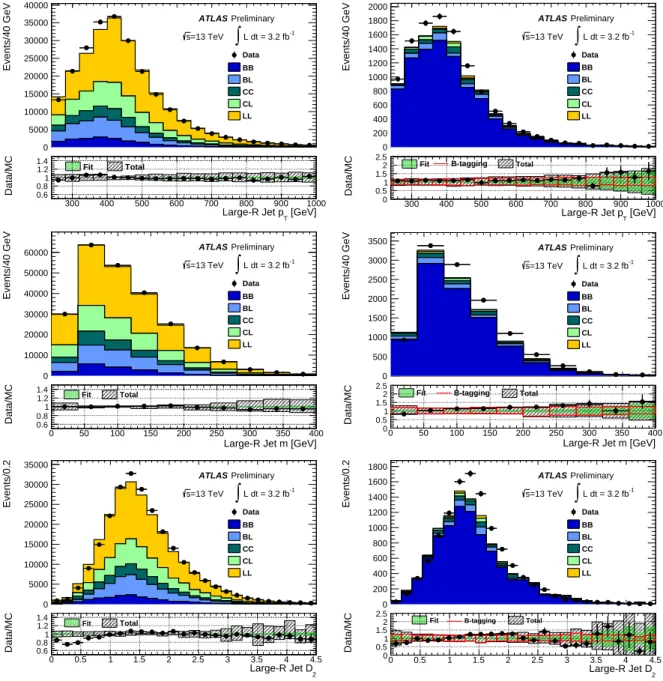
This note follows up on a previous study [11], by improving the expected mass resolution for Higgs boson decays selected in large-Rjets, by refining the Higgs boson selection criteria, and by carrying out a data-to-simulation comparison of large-Rjet properties. After a brief description of the ATLAS detector in Section 2 and of the data and simulated samples in Section 3, the selection as well as association of objects is discussed in Section4, as is the scheme used to label the jets’ truth flavour. The Higgs- jet tagging algorithm and its performance are presented in Section 5. Finally, Section 6 discusses a comparison between representative distributions in a control sample in data dominated byg → bb¯ and corresponding simulated events.

2 ATLAS detector

The ATLAS detector [1] at the LHC covers nearly the entire solid angle around the collision point.¹ It consists of an inner tracking detector surrounded by a thin superconducting solenoid, electromagnetic and hadronic calorimeters, and a muon spectrometer incorporating three large superconducting toroid magnets. The inner-detector system (ID) is immersed in a 2 T axial magnetic field and provides charged particle tracking in the range|η|<2.5.

Preceding data taking at the increased centre-of-mass energy of 13 TeV, the high-granularity silicon pixel detector was equipped with a new barrel layer, located at a smaller radius than the existing layers (at about 34 mm). The upgraded detector covers the vertex region and typically provides four measurements per track, the first hit being normally in the innermost layer. It is followed by the silicon microstrip tracker which usually provides four two-dimensional measurement points per track. These silicon detectors are complemented by the transition radiation tracker, which enables radially extended track reconstruction up to|η|=2.0. The transition radiation tracker also provides electron identification information based on the

1ATLAS uses a right-handed coordinate system with its origin at the nominal interaction point (IP) in the centre of the detector and thez-axis along the beam pipe. The x-axis points from the IP to the centre of the LHC ring, and they-axis points upwards. Cylindrical coordinates (r, φ) are used in the transverse plane,φ being the azimuthal angle around the z-axis.

The pseudorapidity is defined in terms of the polar angleθasη= −ln tan(θ/2). Angular distance is measured in units of

∆R≡p

(∆η)²+(∆φ)².

(3)

fraction of hits (typically 30 in total) above a higher energy deposit threshold corresponding to transition radiation.

The calorimeter system covers the pseudorapidity range|η| < 4.9. Within the region|η| < 3.2, electromagnetic calorimetry is provided by barrel and endcap high-granularity lead/liquid-argon (LAr) electromagnetic calorimeters, with an additional thin LAr presampler covering|η| < 1.8, to correct for energy loss in material upstream of the calorimeters. Hadronic calorimetry is provided by the steel/scintillating- tile calorimeter, segmented into three barrel structures within |η| < 1.7, and two copper/LAr hadronic endcap calorimeters. The solid angle coverage is completed with forward copper/LAr and tungsten/LAr calorimeter modules optimised for electromagnetic and hadronic measurements respectively.

The muon spectrometer (MS) comprises separate trigger and high-precision tracking chambers measuring the deflection of muons in a magnetic field generated by superconducting air-core toroids. The precision chamber system covers the region|η|< 2.7 with three layers of monitored drift tubes, complemented by cathode strip chambers in the forward region, where the background is highest. The muon trigger system covers the range|η|<2.4 with resistive plate chambers in the barrel, and thin gap chambers in the endcap regions.

A two-level trigger system is used to select interesting events [12,13]. The Level-1 trigger is implemented in hardware and uses a subset of detector information to reduce the event rate to a design value of at most 100 kHz. This is followed by the software-based trigger level, the High-Level Trigger (HLT), which reduces the event rate further to about 1 kHz.

3 Data and MC samples

The data used in this note were recorded with the ATLAS detector during the 2015ppcollision run, and correspond to a total integrated luminosity of 3.2 fb⁻¹at √

s=13 TeV. The uncertainty in the integrated luminosity is±2.1%. It is derived, following a methodology similar to that detailed in Refs. [14] and [15], from a calibration of the luminosity scale using x-y beam-separation scans performed in August 2015.

This integrated luminosity accounts for data quality requirements, which ensure that the ATLAS detector was operating well while the data were recorded. Events are required to have a primary vertex with at least 3 tracks associated, and the highestP

p²_Tvertex is considered as the primary vertex. At HLT level, calorimeter jets are reconstructed using the same anti-ktalgorithm [16] (usingR =0.4) used offline (see Section4); events are selected using single jet triggers with thresholds of 100, 150, 175, 200, 260, 300, 320 and 360 GeV. Events must have been recorded by the highest p_Ttrigger that is fully efficient for the leadingp_TR=0.4 offline jet in the event.

Several Monte Carlo (MC) simulated samples are used for the optimisation of the Higgs tagger, the estimation of its performance, and the comparison between data and simulation of its features.

A broad Higgs boson p_T spectrum, withH → bb, is generated as decay products of Randall-Sundrum¯ gravitons of different masses in a benchmark model with a warped extra dimension [2]. The events are generated at leading order using the MadGraph5_aMC@NLO generator [17] interfaced with PY- THIA8 [18] for showering and hadronisation. The leading-order NNPDF2.3 parton distribution (PDF) set [19] is used, with the ATLAS A14 [20] tuned modelling of showering and underlying event paramet- risations.

(4)

Samples of top quark pair events, with hadronically decaying top quarks, are generated using POWHEG [21, 22] interfaced to PYTHIA [23], and with the Perugia2012 [24] underlying event tune parameter sets. Fi- nally, an inclusive multijet sample is generated using PYTHIA8, with the leading-order NNPDF2.3 PDF set and the A14 underlying event tune parameter sets. EvtGen[25] is used in all cases to model the decays ofb- andc-flavoured hadrons.

4 Object selection, association and flavour labelling

The selection, the matching criteria or association, and the determination of the heavy flavour content of physics objects for this analysis are described below.

Calorimeter jets:The standard inputs to calorimeter jet reconstruction in ATLAS are topological clusters of calorimeter cell energy deposits [26]. The clusters are considered massless, and are calibrated using the local hadronic cell weighting method. Calorimeter jets reconstructed using FastJet[27,28] with the anti-kt algorithm [16] with distance parameterR = 1.0 (“large-R” jets) andR = 0.4 (“small-R” jets) are used. The trimming algorithm [29], adopted by ATLAS as the standard grooming procedure for anti-kt

jets with R = 1.0, discards the softer components of the jet, including contributions from pile-up and underlying event. For trimming,kt [30] subjets with R_sub = 0.2 are used with a minimum transverse momentum fraction f_cut = 0.05. After this grooming procedure, the jet energy and mass are calibrated using particle-level correction factors derived from simulation [31,38]. Only jets withp_T >250 GeV and pseudorapidity|η|<2.0 are considered in this analysis.

Truth jets: Truth jets are built in simulated events from truth particles with lifetimes greater than 10 picoseconds, except for muons and neutrinos, which are not included. The same jet clustering algorithm used for the calorimeter jets is also used to reconstruct truth jets.

Track jets: Track jets are reconstructed from inner detector tracks using the anti-kt algorithm with a distance parameter ofR=0.2 [10]. The tracks are required to have:

• p_T >0.4 GeV and|η|<2.5;

• at least 7 hits in the silicon detectors (pixel detector+silicon strip detector);

• no more than one hit in the pixel detector that is shared by multiple tracks;

• no more than one missing hit in the pixel detector, where a hit is expected, and no more than two missing hits in the silicon detectors, where a hit is expected;

• a tight match to the hard scatter vertex by requiring that the track is a constituent of the reconstructed hard scatter vertex, or the track longitudinal impact parameter with respect to the hard scatter vertex, z₀, satisfies|z₀sin(θ)|<3 mm, whereθis the the polar angle of the track momentum at the perigee.

Such requirements greatly reduce the number of tracks from pileup vertices whilst being highly efficient for tracks from the hard scatter vertex. Once the track jet axis is determined, a second step of track association is performed in order to collect tracks needed for effectively running theb-hadron identification algorithms described later in this section. Tracks are selected without impact parameter requirements but within a cone whose size depends on jetp_T[33]. Only track jets withp_T >10 GeV,|η|<2.5, and with at least two tracks are used for the analysis. Theb-hadron identification efficiency of track jets is calibrated using Run 2t¯tcandidate data events.

(5)

Muons: Muons are reconstructed from a combination of measurements from the inner detector and the muon spectrometer. They are required to have≥ 3 hits on at least two layers of monitored drift tubes (MDT), except for the|η| < 0.1 region where tracks with at least three hits in one single MDT layer are allowed. The difference between the inner detector and muon spectrometer 1/pmeasurements is required to be below 7 standard deviations. Muons selected for this analysis are required to havep_T >10 GeV and

|η|<2.4.

Ghost association:In events with a dense hadronic environment, there can often be an ambiguity when matching track jets to calorimeter jets. The track jet association to large-Rjets is performed using ghost- association [34–36], which provides a robust matching procedure that makes use of the catchment area of the jet [36]. As a result, matching to jets with irregular boundaries can be achieved in a less ambiguous way than a simple geometric (i.e. ∆R between objects) matching. In this procedure, the “ghosts” are the track jet 4-vectors in the event, with the track jetp_Tset to an infinitesimal amount, essentially only retaining the direction of the track jets. This ensures that jet reconstruction is not altered by the ghosts when the calorimeter clusters plus ghosts are reclustered. The reclustering is then performed using the anti-kt algorithm with R = 1.0. The calorimeter jets after reclustering are identical to the ungroomed parents of the trimmed jets used in this analysis, with the addition of the associated track jets retained as constituents. In this analysis, track jets ghost-associated to the large-Rjet refer to track jets found this way within the catchment area of the ungroomed parent jet, but the kinematics of the large-Rjet are still measured using the trimmed jet.

Jet flavour labelling:The labelling of the flavour of the track jets in simulation is done by geometrically matching the jet with generator-level hadrons: if a weakly decayingb-hadron with p_T > 5 GeV is found within∆R<0.2 of the jet direction, whereRis the jet distance parameter, the jet is labelled as ab-jet. In the case that theb-hadron could match more than one jet, only the closest jet is labelled as ab-jet. If no b-hadron is found, the procedure is repeated for weakly decayingc-hadrons to labelc-jets. If noc-hadron is found, the procedure is repeated forτleptons to labelτ-jets. A jet for which no such association can be made is labelled as a light-flavour jet.

The flavour labelling for large-R jets is also important for this analysis to define the Higgs-jet signal and background efficiencies. Higgs-jets are defined as large-R jets with a truth Higgs boson and the corresponding two decayb-hadrons found within∆R< 1. Top jets are defined as large-Rjets in which a truth top quark is found within∆R<1 of the large-Rjet axis.

b-jet identification:Several algorithms to identifyb-jets have been developed based on the lifetime and decay properties ofb-hadrons [33]. Tracks that are associated to the jets and that pass basic quality requirements are used as inputs to the algorithms. The algorithms use relatively simple impact parameter (IP3D) and secondary vertex (SV1) information, or, in the case of the more refined JetFitter algorithm, exploit the topology of weakb- andc-hadron decays using a Kalman filter to search for a common line connecting the primary vertex to beauty and charm decay vertices.

The MV2c10 algorithm [33,37] employs a boosted decision tree based on jet properties and properties computed from IP3D, SV1 and JetFitter. It is trained withb-jets as signal, and a mix of approximately 93% light-flavour jets and 7%c-jets as background. The multivariate b-tagging algorithms have been trained usingR=0.4 calorimeter jets, but they are used for both calorimeter and track jets.

For a jet to be consideredb-tagged, the output of the multivariateb-tagging algorithm is required to be above a fixed threshold value. Several such thresholds, or “working points” (WP), are defined, in such a way as to correspond to a well-defined average efficiency when applied to b-jets from a sample of

(6)

inclusivet¯tevents. In this note, emphasis will be placed on WP that are tuned to an average 70% and 77%b-tagging efficiency.

Large-Rjet mass:An independent estimate of the invariant mass of large-Rjets, intended to overcome the limited angular resolution provided by the calorimeter, is obtained as the so-called "track-assisted jet mass"m^TA[38] which is computed asm^TA =m^track× p^calo_T /p^trk_T , wherem^trackis the invariant mass of the tracks associated with the trimmed large-Rjet reconstructed using the calorimeter, p^calo_T is the transverse momentum of the trimmed large-R jet reconstructed using the calorimeter, and p^track_T is the transverse momentum of the sum over the four-momenta of associated tracks. The correction factor p^calo_T /p^track_T corrects for the neutral jet component, to whichm^track is not sensitive. The track-assisted jet mass is calibrated using particle-level correction factors derived from simulation [38] as for calorimeter jets.

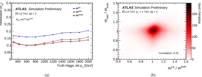
As shown in Figure1(a), the resolution in the response to jet mass R_m = m_reco/mtruth provided bym^TA is compared to the jet mass reconstructed using the calorimeterm^caloas a function of truth Higgs-jetp_T. The truth jet massm_truthis the invariant mass of particles clustered into truth trimmed large-Rjets. The relative jet mass resolution is defined as half the central 68% probability interval divided by the median of the jet mass response distribution. Them^calo observable provides better resolution thanm^TAover the entire p_T range considered. Both the calorimeter-based and track-assisted jet mass resolution degrade for p_T > 800 GeV. For m^calo this is due to the finite granularity of the calorimeter; form^TA it is due to a degrading track momentum resolution and to a loss of tracks in the high density jet core caused by overlapping hits [38]. The tracks from theb-hadron decays are expected to have high transverse momenta since they carry a large fraction of theb-quark momentum due to the hard b-quark fragmentation. In addition, for the same large-R jet p_T, the decay products of the Higgs boson are more separated than those ofW andZ bosons due to the higher Higgs boson mass, resulting in a slower degradation of the resolution inm^calotowards higher jetp_Tfor Higgs-jet.

The statistical correlation between them^calo andm^TA measurements is modest (with linear correlation coefficientρ∼0.23 for jets withp_T >1 TeV, as can be seen in Figure1(b)), and therefore an uncertainty- weighted combination of the two variables, denoted asm^comb, is expected to result in an improved resolution. Them^combresolution is found to be compatible with them^caloresolution at Higgs-jet p_T below 600 GeV, with a resolution gain improving by up to 10% for a p_Tof 2 TeV. Figure2(a)shows the calibrated large-Rjet mass distributions,m^caloandm^TA, including the muon correction discussed below, in the jet transverse momentum ranges of 350 GeV< p_T <500 GeV and 1000 GeV< p_T <1500 GeV.

The particle-level correction factors mentioned above do not account for semi-muonic decays, which occur in approximately 20% of allb-hadron decay chains. As the resulting neutrinos are not measured directly by the detector, only the muons are considered. The effect of these decays is corrected by finding muons within∆R < 0.2 of theb-tagged track jets and adding the four vector of these muons to that of the large-Rcalorimeter jet (while taking into account the muon energy loss in the calorimeter). If more than one muon is found within a track jet, only the muon closest to the track jet axis is considered. In case of m^TA only the jet calorimeter measurement of the jet p_T is corrected. The m^calo andm^TA mass distributions of the large-RHiggs jets are shown in Figure2(b)before and after the muon correction in the 350 GeV < p_T < 500 GeV range. The mass resolution of Higgs-jets is clearly improved in both cases at low Higgs-jetp_T, while the improvement is not as pronounced at higher p_Tas has been shown in Ref. [11].

Given the limited improvement obtained from combining the calorimeter-based jet mass definitionm^calo with the track-assisted jet massm^TA, them^calodefinition is used throughout the note. The muon correction is added on top.

(7)

[GeV]

Truth Higgs Jet pT

400 600 800 1000 1200 1400 1600 1800 2000 )mResolution (R

0 0.05 0.1 0.15 0.2 0.25 0.3 0.35 0.4

mTA

mcalo

mcomb

ATLAS Simulation Preliminary

| < 2 η

=13 TeV, | s

truth reco/m

m=m R

(a)

truth TA / m m

0.4 0.6 0.8 1 1.2 1.4 1.6

truth / mcalom

0.4 0.6 0.8 1 1.2 1.4 1.6

Arbitrary Units

0 50 100 150 200 ATLAS Simulation Preliminary

| < 2 η > 1 TeV, |

=13 TeV, pT

s

Correlation: 0.23

(b)

Figure 1: (a) The resolution in the response of invariant mass of large-R Higgs-jetsRm = _m^m_truth^reco as a function of the transverse momentum pT of the Higgs-jet for|η| <2. The resolution is defined here as half the central 68%

probability interval divided by the median of the jet mass response distribution. (b) The correlation between the responses in them^calo andm^TAobservables for large-RHiggs-jets with pT >1 TeV and within|η|<2. The muon corrections described in the text are applied.

Jet mass [GeV]

60 80 100 120 140 160 180 200

Normalised to unity

0 0.01 0.02 0.03 0.04 0.05 0.06 0.07 0.08

| < 2 η

=13 TeV, | s

< 500 GeV : 350 < pT

mcalo

< 500 GeV : 350 < pT

mTA

< 1500 GeV : 1000 < pT

mcalo

< 1500 GeV : 1000 < pT

mTA

(a)

Jet mass [GeV]

60 80 100 120 140 160 180 200

Normalised to unity

0 0.01 0.02 0.03 0.04 0.05 0.06 0.07 0.08

| < 2 η

=13 TeV, | s

< 500 GeV 350 < pT

mcalo

muon corrected mcalo

mTA

muon corrected mTA

(b)

Figure 2: (a) The calibrated large-Rjet mass distributions,m^caloandm^TA, after the muon correction described in the text, are shown in the large-Rjet transverse momentum ranges of 350 GeV<pT <500 GeV and 1000 GeV<pT<

1500 GeV. (b) The calibrated large-Rjet mass distributions,m^caloandm^TA, before and after the muon correction, are shown in the jet transverse momentum range of 350 GeV<pT<500 GeV.

(8)

[GeV]

Truth Higgs pT

400 600 800 1000 1200 1400 1600 1800 2000

Truth Higgs Acceptance

0 0.2 0.4 0.6 0.8 1 1.2 1.4 1.6 1.8 2

Simulation Preliminary ATLAS

MV2c10 b-tagging at 77% WP

| < 2.0

jet

ηdet

> 250 GeV, |

jet

pT

| < 2.0

Higgs

ηtrue

|

| < 2.5

b

ηtrue

> 5 GeV, |

b T,true

p

Baseline selection window

jet

1 b-tag, Loose mcalo

selection

jet

2 b-tags, No mcalo

window

jet

2 b-tags, Loose mcalo

sel.

window, D2 jet

2 b-tags, Tight mcalo

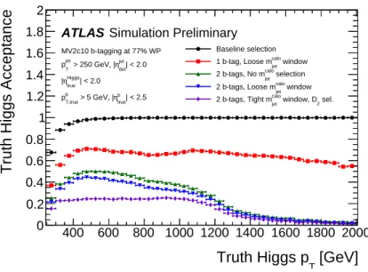
Figure 3: Truth Higgs boson acceptance, defined as the fraction of truth Higgs bosons with|η|<2.0, and withb- hadrons from the Higgs boson decay withpT>5 GeV and|η|<2.5, that are associated to the reconstructed large-R jets after the baseline selection defined in Section4. The effects of additional Higgs-jet tagging requirements are shown as additional curves.

5 Higgs-jet tagger

In this section, the Higgs-jet tagging procedure is described and its performance in terms of tagging efficiency and background rejection is discussed. The Higgs-jet tagging consists of the following steps:

• track jetb-tagging

• large-Rjet mass window cut around the Higgs boson mass peak

• cut on large-Rjet substructure variables

The first step in identifying boosted Higgs bosons is the large-R jet reconstruction. The acceptance of this reconstruction step, defined as the fraction of truth Higgs bosons with p_T > 250 GeV,|η|< 2.0, and withb-hadrons from the Higgs boson decay withp_T > 5 GeV and|η| < 2.5, that are reconstructed with the baseline large-Rjet selection and labelled as a Higgs-jet (using the selection and labelling criteria defined in Section4), is shown as a function of truth Higgs bosonp_T in Figure3. The angular separation between the decay products of the Higgs boson can be approximated by∆R ≈ ^2m_p^H

T , thus only for Higgs boson p_T values above 250 GeV its decay products will be collimated within ∆R . 1.0, i.e. within a single large-Rjet. This acceptance increases rapidly with Higgs boson p_T, reaching more than 95% for p_T >400 GeV.

The large-Rjet p_T of signal and background samples differ. Therefore, for the performance studies and optimisations discussed in this note, the signal samples are summed together and reweighted to the jet p_T distribution of the multi-jet sample. The same procedure is applied to the hadronict¯tsamples. In the following subsections, the Higgs-jet tagging efficiency is defined as the number of Higgs-jets passing a given selection requirement divided by the total number of Higgs-jets passing the baseline selection

(9)

defined in Section4. The background rejection is defined as the inverse of the efficiency for a background jet to pass the requirement.

5.1 Track jetb-tagging performance

Theb-tagging for large-Rjets is performed by means of the ghost associated track jets. The track jets are always ordered by p_T, and only the leading two track jets (if they exist) are used for double and asymmetricb-tagging. For singleb-tagging benchmarks only one track jet associated to the large-Rjet is required. A track jet is considered to have passed theb-tagging requirement if the track jet’s MV2c10 b-tagging weight,w_b−tag, is larger than a threshold value,wX. The value ofwXcan be scanned to examine the background rejection as a function of Higgs-jet efficiency for differentb-tagging requirements.

Several differentb-tagging requirements on the track jets are examined:

• Double b-tagging: the two leading p_Ttrack jets must both pass the sameb-tagging requirement of havingw_b−tag> wX.

• Asymmetric (Asymm.) b-tagging: Of the two leading p_T track jets, the track jet with the largest b-tagging weight must pass the fixed 60%, 70%, 77% or 85%b-tagging working point threshold, e.g.w_b−tag> w_70%, while theb-tagging requirement of the other jet is varied.

• Leading subjet single b-tagging: only the leading p_Ttrack jet must pass theb-tagging requirement of havingw_b−tag> wX.

• Single b-tagging: at least one of the two leadingp_Ttrack jets must pass theb-tagging requirement of havingwb−tag> wX.

The Higgs-jet efficiency versus the inclusive multi-jet rejection can be found in Figure4(a), where the performance of all benchmarks is shown. The double and asymmetricb-tagging curves do not reach a Higgs-jet efficiency of 100% due to a requirement of at least two track jets needed for doubleb-tagging (the baseline selection requires only one track jet) and, in the case of asymmetricb-tagging, due also to the fixedb-tagging working point requirement on one of the track jets. The background rejection of singleb-tagging is larger than that of the leading subjet singleb-tagging in general and especially for high signal efficiencies. For high Higgs-jet efficiencies, above∼ 75%, a high doubleb-tagging efficiency is only possible at the expense of a high tagging efficiency for individual light-flavour jets, and the single b-tagging approach tends to have a better multi-jet rejection than the doubleb-tagging. For lower Higgs- jet efficiency the doubleb-tagging approach provides a significantly higher multi-jet rejection. Finally, the asymmetricb-tagging option is seen to capture much of the benefits of doubleb-tagging in the low Higgs-jet efficiency regime, while being significantly better than both single and doubleb-tagging in the high Higgs-jet efficiency regime except at very high efficiencies above∼90%, where the singleb-tagging approach shows the best performance.

While Figure4(a) includes all large-Rjets with p_T > 250 GeV, Figure4(b) shows the performance of b-tagging requirements for large-Rjet p_T above 1 TeV. In thisp_Tregime, the singleb-tagging approach has the best performance already at signal efficiencies above∼55%, while the double and asymmetricb- tagging options have a similar performance below∼25%. In the signal efficiency range between∼ 25%

and∼55%, the asymmetricb-tagging approach has the best background rejection.

Another common background to boosted Higgs boson searches are boosted hadronic top-quark decays.

The inclusive hadronic top jet rejection versus the Higgs-jet efficiency can be found in Figure4(c), where

(10)

Higgs-jet efficiency

0.1 0.2 0.3 0.4 0.5 0.6 0.7 0.8 0.9 1

Multi-jet rejection

1 10 102

103

104

105

106

selection

jet

> 250 GeV, No mcalo T

p

Double b-tag Asymm. b-tag (70% wp) Single b-tag Leading subjet b-tag

(a)

0.1 0.2 0.3 0.4 0.5 0.6 0.7 0.8 0.9 1

Multi-jet rejection

1 10 102

103

104

105

106

selection

jet

p

(b)

0.1 0.2 0.3 0.4 0.5 0.6 0.7 0.8 0.9 1

Hadronic top rejection

1 10 102

103

104

105

106

selection jet > 250 GeV, No mcalo pT

(c)

0.1 0.2 0.3 0.4 0.5 0.6 0.7 0.8 0.9 1

1 10 102

103

104

105

106

selection

jet

p

(d)

Figure 4: (a) The rejection of inclusive multi-jets versus Higgs-jet efficiency using large-Rjets withpT>250 GeV, for variousb-tagging requirements. (b) Same as (a) but using large-Rjets withpT >1000 GeV. (c) Hadronic top background rejection versus Higgs-jet efficiency using all large-Rjets withpT >250 GeV, for variousb-tagging requirements. (d) Same as (c) but using large-Rjets with pT >1000 GeV. The stars correspond to the 60%, 70%, 77% and 85%b-tagging WPs (from left to right).

(11)

the performance of doubleb-tagging, singleb-tagging and asymmetricb-tagging is shown. Double and asymmetric b-tagging perform similarly and both provide significantly better rejection than single b- tagging with no significant loss in Higgs-jet efficiency. Only for very high Higgs-jet efficiencies, above

∼85%, the singleb-tagging approach has a higher background rejection than the double and asymmetric b-tagging options. Figure 4(d) shows the hadronic top jet rejection for large-Rjet p_T above 1 TeV. A similar behaviour as for the multi-jet rejection is observed: the singleb-tagging approach has the best performance above 55% signal efficiency, for lower signal efficiencies the double and asymmetric b- tagging show a better background rejection.

5.2 Mass window and substructure requirements

The groomed and muon corrected calorimeter reconstructed massm^calo is an important component in tagging boson jets [11]. A mass window requirement, selecting a range of masses around the Higgs boson mass, is applied. The 93–134 GeV and 76–146 GeV intervals are used as the smallest intervals containing approximately 68% (“tight mass window cut”) and 90% (“loose mass window cut”) of the groomed Higgs-jet mass distributions, respectively. The mass intervals are derived for the Higgs-jet sample integrated over the fullp_T spectrum.

Figure5 shows the Higgs tagging performance for the sameb-tagging benchmarks as in Figure 4 but adding the loose and tight mass window requirements. The conclusions are similar to the ones described in the previous section.

In addition to the heavy flavour content of the large-Rjet, and the jet mass, the internal structure of the jet can be used to discriminate Higgs-jets from multi-jet production and hadronic top decays. There are a large number of substructure variables that capture features of a jet’s internal structure. D^(β₂⁼¹⁾[39,40]

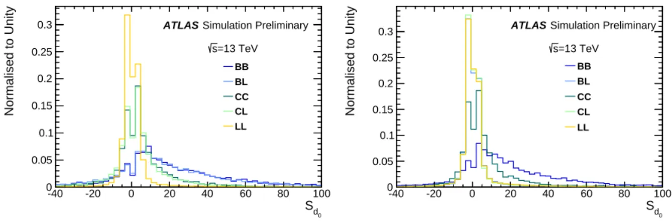
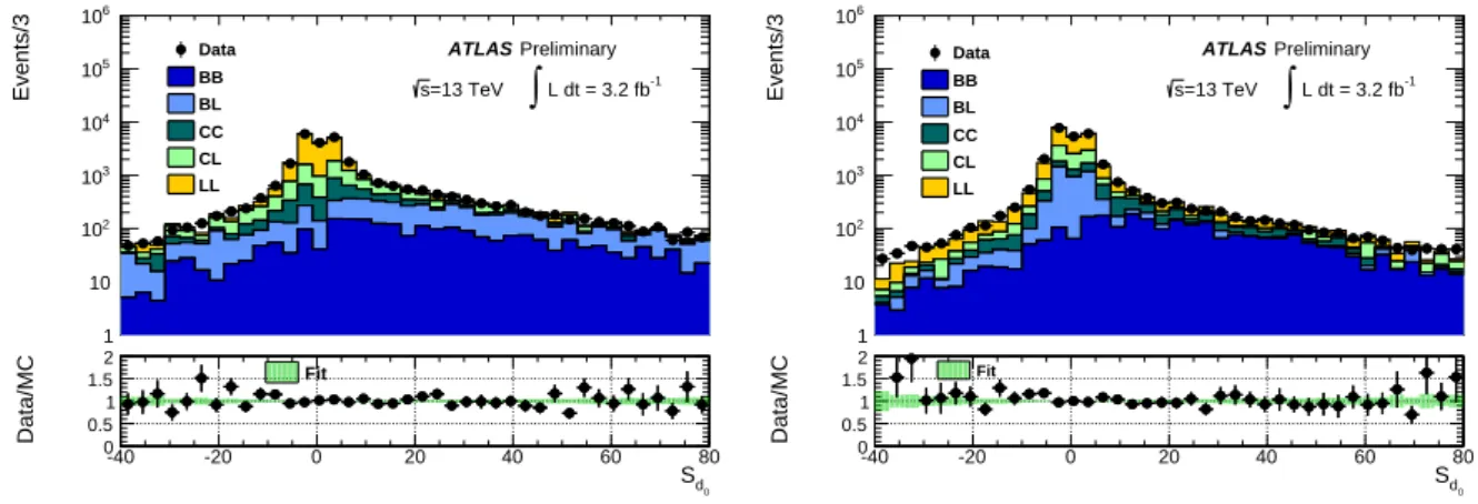
is used in this analysis, defined as a ratio of the two and three point energy correlation functions, which are based on the energies and pair-wise angular distances of particles within a jet. This variable was optimised to separate between one-prong and two-prong decays. A detailed description can be found in Ref. [32]. Previous studies [9,32,41] have shown that this variable is one of the most sensitive for this topology; in addition, calibration as well as resolution and scale uncertainties have been derived for this variable. Ap_T dependent selection identical to the one of Ref. [11] is applied here.

5.3 Systematic uncertainties of the Higgs-jet tagger performance

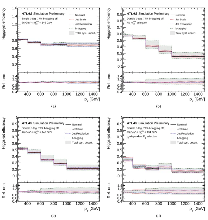
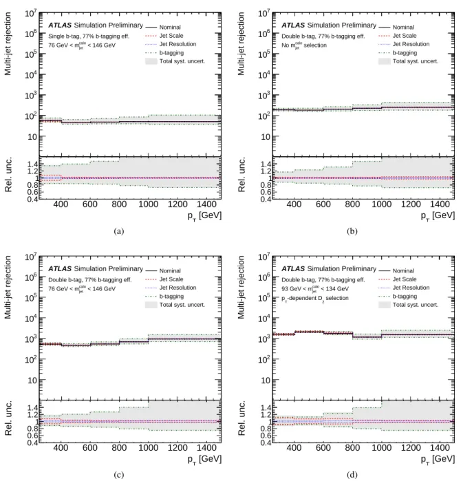
To estimate the experimental systematic uncertainties of the Higgs-jet tagger performance, the uncertainties on the Higgs-jet tagger inputs are propagated through the tagger selection. More specifically, the b-tagging efficiency and the jet mass, p_T, and D^(β₂⁼¹⁾ scale and resolutions are varied within their uncertainties [38]. These input uncertainties lead to changes in the efficiency or acceptance or both of the Higgs-jet tagger selection, and thus provide an estimate of the systematics uncertainties of the Higgs-jet efficiency and background rejection.

Figures6,7and8show the Higgs-jet tagging efficiency and background rejection, including the effect of various systematic uncertainties. The largest uncertainty is theb-tagging uncertainty, especially for the doubleb-tagging working point; the jet related systematics become larger at very high jet p_T. Figure9 shows the Higgs-jet tagging efficiency and background rejection for all benchmarks defined in5.1. The total uncertainty is the sum in quadrature of the statistical and systematic uncertainties.

(12)

0.1 0.2 0.3 0.4 0.5 0.6 0.7 0.8 0.9 1

Multi-jet rejection

1 10 102

103

104

105

106

< 146 GeV jet > 250 GeV, 76 GeV < mcalo pT

(a)

0.1 0.2 0.3 0.4 0.5 0.6 0.7 0.8 0.9 1

Multi-jet rejection

1 10 102

103

104

105

106

< 134 GeV

jet

> 250 GeV, 93 GeV < mcalo T

p

(b)

0.1 0.2 0.3 0.4 0.5 0.6 0.7 0.8 0.9 1

Multi-jet rejection

1 10 102

103

104

105

106

< 146 GeV

jet

> 1000 GeV, 76 GeV < mcalo

pT

(c)

0.1 0.2 0.3 0.4 0.5 0.6 0.7 0.8 0.9 1

Multi-jet rejection

1 10 102

103

104

105

106

< 134 GeV

jet

pT

(d)

0.1 0.2 0.3 0.4 0.5 0.6 0.7 0.8 0.9 1

1 10 102

103

104

105

106

< 146 GeV

jet

pT

(e)

0.1 0.2 0.3 0.4 0.5 0.6 0.7 0.8 0.9 1

1 10 102

103

104

105

106

< 134 GeV

jet

pT

(f)

Figure 5: Top: The rejection of inclusive multi-jet background versus Higgs-jet efficiency using large-Rjets with pT >250 GeV for variousb-tagging requirements using loose (a) and tight (b) mass window cuts. Middle: Same as above, but using all large-Rjets withpT >1000 GeV. Bottom: Hadronic top background rejection versus Higgs-jet efficiency using all large-Rjets withpT>250 GeV for variousb-tagging requirements using loose (e) and tight (f) mass window cuts. The stars correspond to the 60%, 70%, 77% and 85%b-tagging WPs (from left to right).

(13)

[GeV]

pT

400 600 800 1000 1200 1400

0.2 0.4 0.6 0.8 1 1.2 1.4 1.6

Single b-tag, 77% b-tagging eff.

< 146 GeV

jet

76 GeV < mcalo

Nominal Jet Scale Jet Resolution b-tagging Total syst. uncert.

[GeV]

pT

400 600 800 1000 1200 1400

Rel. unc.

0.4 0.60.81 1.21.4

Rel. unc.

(a)

[GeV]

pT

400 600 800 1000 1200 1400

0.1 0.2 0.3 0.4 0.5 0.6 0.7 0.8 0.9 1

Double b-tag, 77% b-tagging eff.

selection

jet

No mcalo

[GeV]

pT

400 600 800 1000 1200 1400

Rel. unc.

0.4 0.60.81 1.21.4

Rel. unc.

(b)

[GeV]

pT

400 600 800 1000 1200 1400

0.1 0.2 0.3 0.4 0.5 0.6 0.7 0.8 0.9 1

< 146 GeV

jet

76 GeV < mcalo

[GeV]

pT

400 600 800 1000 1200 1400

Rel. unc.

0.40.6 0.81 1.21.4

Rel. unc.

(c)

[GeV]

pT

400 600 800 1000 1200 1400

0.1 0.2 0.3 0.4 0.5 0.6 0.7 0.8 0.9 1

< 134 GeV

jet

93 GeV < mcalo

selection -dependent D2

pT

[GeV]

pT

400 600 800 1000 1200 1400

Rel. unc.

0.40.6 0.81 1.21.4

Rel. unc.

(d)

Figure 6: Higgs-jet signal efficiency as a function of the pT of large-R jets using the 77% b-tagging WP, and requiring various Higgs-jet mass window cuts andb-tagging requirements: (a) at least one associatedb-tagged track jet and a loose mass window cut, (b) two associatedb-tagged track jets and no mass window cut, (c) two associatedb-tagged track jets and a loose mass window cut, (d) two associatedb-tagged track jets, a tight mass window cut and a cut onD^(β₂⁼¹⁾.

(14)

[GeV]

pT

400 600 800 1000 1200 1400

10 102

103

104

105

106

107

< 146 GeV

jet

76 GeV < mcalo

[GeV]

pT

400 600 800 1000 1200 1400

Rel. unc.

0.4 0.60.81 1.21.4

Rel. unc.

(a)

[GeV]

pT

400 600 800 1000 1200 1400

10 102

103

104

105

106

107

selection

jet

No mcalo

[GeV]

pT

400 600 800 1000 1200 1400

Rel. unc.

0.4 0.60.81 1.21.4

Rel. unc.

(b)

[GeV]

pT

400 600 800 1000 1200 1400

10 102

103

104

105

106

107

< 146 GeV

jet

76 GeV < mcalo

[GeV]

pT

400 600 800 1000 1200 1400

Rel. unc.

0.40.6 0.81 1.21.4

Rel. unc.

(c)

[GeV]

pT

400 600 800 1000 1200 1400

10 102

103

104

105

106

107

< 134 GeV

jet

93 GeV < mcalo

pT

[GeV]

pT

400 600 800 1000 1200 1400

Rel. unc.

0.40.6 0.81 1.21.4

Rel. unc.

(d)

Figure 7: Hadronic top background rejection as a function of the pT of large-Rjets using the 77%b-tagging WP, and requiring various Higgs-jet mass window cuts andb-tagging requirements: (a) at least one associatedb-tagged track jet and a loose mass window cut, (b) two associatedb-tagged track jets and no mass window cut, (c) two associatedb-tagged track jets and a loose mass window cut, (d) two associatedb-tagged track jets, a tight mass window cut and a cut onD^(β₂⁼¹⁾.

(15)

[GeV]

pT

400 600 800 1000 1200 1400

Multi-jet rejection

10 102

103

104

105

106

107

< 146 GeV

jet

76 GeV < mcalo

[GeV]

pT

400 600 800 1000 1200 1400

Rel. unc.

0.4 0.60.81 1.21.4

Rel. unc.

(a)

[GeV]

pT

400 600 800 1000 1200 1400

Multi-jet rejection

10 102

103

104

105

106

107

selection

jet

No mcalo

[GeV]

pT

400 600 800 1000 1200 1400

Rel. unc.

0.4 0.60.81 1.21.4

Rel. unc.

(b)

[GeV]

pT

400 600 800 1000 1200 1400

Multi-jet rejection

10 102

103

104

105

106

107

< 146 GeV

jet

76 GeV < mcalo

[GeV]

pT

400 600 800 1000 1200 1400

Rel. unc.

0.40.6 0.81 1.21.4

Rel. unc.

(c)

[GeV]

pT

400 600 800 1000 1200 1400

Multi-jet rejection

10 102

103

104

105

106

107

< 134 GeV

jet

93 GeV < mcalo

pT

[GeV]

pT

400 600 800 1000 1200 1400

Rel. unc.

0.40.6 0.81 1.21.4

Rel. unc.

(d)

Figure 8: Multi-jet background rejection as a function of the pT of large-Rjets using the 77%b-tagging WP, and requiring various Higgs-jet mass window cuts andb-tagging requirements: (a) at least one associatedb-tagged track jet and a loose mass window cut, (b) two associatedb-tagged track jets and no mass window cut, (c) two associated b-tagged track jets and a loose mass window cut, (d) two associatedb-tagged track jets, a tight mass window cut and a cut onD^(β₂⁼¹⁾.

(16)

[GeV]

pT

400 600 800 1000 1200 1400

0 0.2 0.4 0.6 0.8 1 1.2 1.4 1.6

MV2c10 b-tagging at 77% WP jet^window

1 b-tag, Loose mcalo selection jet 2 b-tags, No mcalo

window jet 2 b-tags, Loose mcalo

sel.

window, D2 jet 2 b-tags, Tight mcalo

(a)

[GeV]

pT

400 600 800 1000 1200 1400

Multi-jet rejection

1 10 102

103

104

105

106

107

sel.

(b)

[GeV]

pT

400 600 800 1000 1200 1400

1 10 102

103

104

105

106

107

sel.

(c)

Figure 9: (a) Higgs-jet signal efficiency, (b) Multi-jet background rejection and (c) Hadronic top background rejection as a function of thepTof large-Rjets with one or two associatedb-tagged track jets, using the 77%b-tagging WP, and requiring various Higgs-jet mass window cuts and a cut onD^(β₂⁼¹⁾.