ATLAS-CONF-2018-022 08June2018
ATLAS CONF Note
ATLAS-CONF-2018-022
8th June 2018
Measurement of the Jet Vertex Charge algorithm performance for identified b -jets in t t ¯ events
in p p collisions with the ATLAS detector
The ATLAS Collaboration
The Jet Vertex Charge algorithm, developed recently within the ATLAS collaboration, dis- criminates between jets resulting from the hadronisation of a bottom quark or bottom an- tiquark. This note describes a measurement of the performance of the algorithm and the extraction of data-to-simulation scale factors, made using b-tagged jets in candidate single leptontt¯events. The data sample was collected by the ATLAS detector at the LHC usingpp collisions at
√s= 13 TeV in 2015 and 2016 and corresponds to a total integrated luminosity of 36.1 fb−1. Overall, good agreement is found between data and the simulation.
© 2018 CERN for the benefit of the ATLAS Collaboration.
Reproduction of this article or parts of it is allowed as specified in the CC-BY-4.0 license.
1 Introduction
Final states with jets containingb-hadrons, calledb-jets, arise from a variety of different processes, either in the context of Standard Model, such as in a top quark decay or in more complex final state asH→bb¯ produced in association with at¯tpair, or in scenarios predicted in extensions of the Standard Model. In general, multipleb-jets may be present in such final states, and the resulting combinatorics complicate the full event reconstruction.
Due to the hadronisation of theb- (anti)quarks as well as subsequent (neutral) B-meson oscillations, it is not possible to measure the b-quark electric charges directly. However, it is possible to exploit various properties ofb-jets to indirectly extract this information. The Jet Vertex Charge (JVC) algorithm [1] has been developed within the ATLAS collaboration for this purpose, as exploiting the electric charge ofb-jets can improve the full event reconstruction of complex final states and hence improve analyses. It exploits inclusive jet properties such as thejet charge[2], i.e., the sum of the charges of the reconstructed charged particles weighted by powers of their transverse momenta,pT, which has also been used in other ATLAS analyses [3–5]. In addition, the JVC algorithm uses information relevant to the identification ofb-jets. In particular, two different charges are constructed, based on the possibility to reconstruct a secondary (SV) and a tertiary vertex (TV) inside the jet with the JetFitter algorithm [6]. Finally, the charge of any muon found within the jet, if present, is used.
Based on the availability of the charge information, jets are classified in different categories. In categories where two or more vertex charges are available, a neutral network is trained using those variables as input, together with a set of auxiliary variables that are used by the network to discriminate poorly reconstructed displaced vertices from well reconstructed ones. Vertex reconstruction quality, track multiplicity at the vertex or quantities describing the muon are examples of such variables. In the categories where only one charge variable is available, that variable is used for the identification of the charge of the jet. For each category, the finalλJVC variable is computed as the logarithm of the ratio of the discriminant probability densities under the hypotheses that the jet originated from the decay of either a ¯b- or a b-quark. A description of the algorithm is given in Ref. [1].
This note describes a measurement of the performance of the JVC algorithm for b-jets, carried out in a sample oftt¯candidate events with a single identified and isolated charged lepton (e or µ), and with two identifiedb-jets. In such events, sufficient kinematic constraints exist to allow for an unambiguous reconstruction of thet¯tsystem. The charge of the lepton then provides a very clean reference to compare the reconstructedλJVCdistribution of theb-jet of the leptonic top quark decay topology between data and simulated events. Finally, this comparison allows for the extraction of data-to-simulation scale factors (SF), which can be used to correct the simulated λJVC distribution in analyses aiming to exploit this observable.
Calibrating the binned λJVC distribution implies that it can be used in analyses in a variety of ways.
Examples include labelling all theb-tagged jets with a value of |λJVC| > λcutor, alternatively, using the binned distribution as an input into a multivariate algorithm.
The present note is organised as follows. Sections2and3describe the ATLAS detector and the data and simulated samples, respectively. The reconstruction of objects is described in Section4, while Section5 details the event selection and the reconstruction of thet¯tsystem. The analysis is presented in Section6, while the associated systematic uncertainties are discussed in Section7.
2 The ATLAS detector
The ATLAS detector [7] is a general-purpose particle physics detector with a forward-backward symmetric cylindrical geometry and a near 4πcoverage in solid angle.1ATLAS consists of an inner tracking detector (ID) surrounded by a 2 T superconducting solenoid, electromagnetic and hadronic calorimeters, and a muon spectrometer (MS) with a toroidal magnetic field of bending power between 1 Tm and 7.5 Tm.
The ID provides charged-particle tracking for |η| <2.5. It consists of silicon pixel and strip detectors surrounded by a straw tube tracker (TRT), which also provides transition radiation measurements for electron identification. A new detector, the Insertable B-Layer (IBL), has been installed at a mean sensor radius of 3.2 cm from the beam line [8], improving the impact parameter resolution for charged-particle tracks and the reconstruction of displaced vertices. The calorimeter system covers pseudorapidities up to|η| <4.9. A finely segmented sampling calorimeter using lead/liquid argon provides electromagnetic energy measurements up to |η| < 3.2 and a hadronic calorimeter consisting of steel tiles and plastic scintillators provides hadronic energy measurements in the central pseudorapidity region |η| < 1.7. In the pseudorapidity range 1.5 < |η| < 4.9, a sampling calorimeter using tungsten/liquid argon provides hadronic energy measurements. The MS covers the range|η|< 2.7.
The ATLAS detector consists of a two-level trigger system. The first level is implemented in custom hardware and uses the calorimeter and muon systems to reduce the accepted event rate to 100 kHz. The L1 trigger is followed by a software based high-level trigger (HLT) to reduce the accepted event rate to approximately 1 kHz for offline analysis [9].
3 Data and simulated event samples
This analysis is based on data recorded by the ATLAS detector in LHC proton-proton collisions at a centre- of-mass energy
√s= 13 TeV in 2015 and 2016. Only events recorded during stable beam conditions and satisfying detector and data-quality requirements are considered, resulting in a total integrated luminosity of 36.1 fb−1.
Events were collected using single-electron and single-muon triggers. Due to the increase in instantaneous luminosity between the 2015 and 2016 data periods, the triggers used in the analysis have higher pT thresholds during the 2016 period.
For the 2015 dataset, the single-electron trigger used apTthreshold of 24 GeV, with additional identification and isolation criteria applied. At highpTmore relaxed isolation criteria were applied. Similarly, the single- muon trigger used a pT threshold of 20 GeV and a loose isolation criterion. At high pT, the isolation criteria were again relaxed. In the 2016 dataset, the triggerpTthresholds used were raised to 26 GeV for both electrons and muons; in addition, their isolation criteria were tightened.
The simulated samples used in this analysis are described below. All generated events are passed through a Geant4 [10] based software to simulate the response of the ATLAS detector [11]. A fast simulation was adopted for the samples used to estimate thett¯modelling systematic uncertainties, where the full
1ATLAS uses a right-handed coordinate system with its origin at the nominal interaction point (IP) in the centre of the detector and the z-axis along the beam line. The x-axis points from the IP to the centre of the LHC ring, and they-axis points upwards. Cylindrical coordinates(r, φ) are used in the transverse plane, φbeing the azimuthal angle around the z-axis.
The pseudorapidity is defined in terms of the polar angleθasη =−ln tan(θ/2). Angular distance is measured in units of
∆R≡
q(∆η)2+(∆φ)2.
simulation of the calorimeter response is replaced by a detailed parametrisation of the shower shapes [12].
Effects of multipleppinteractions in the same and neighbouring bunch crossings, denoted as pile-up, are accounted for by overlaying each event with a variable number of inelasticppinteractions generated using Pythia 8.1 [13] with the A2 tuned parameters of the Monte Carlo programs [14]. Eachppinteraction of the simulated samples is then re-weighted to reflect the distribution of the average number ofppcollisions in data. Simulated events are subsequently reconstructed using the same program as for the data.
3.1 Inclusivett¯
The nominalt¯tsample is generated using the Powheg-Box v2 next-to-leading order (NLO) generator [15–
17] with the NNPDF3.0 parton distribution function (PDF) set [18]. Thehdampparameter, which controls thepTof the first additional emission beyond the Born configuration, is set to 1.5 times the top quark mass ofmt =172.5 GeV. The parton shower and hadronisation processes are modelled by Pythia 8.2 [19] with the A14 [20] set of tuned parameters. The EvtGen v1.2.0 [21] program is used to simulate the bottom and charm hadron decays. The sample is normalised to the Top++2.0 [22] theoretical cross section of 832+46−51pb, calculated at next-to-next-to-leading order (NNLO) in QCD, which includes resummation of next-to-next-to-leading logarithmic (NNLL) soft gluon terms [23–27].
Alternative tt¯ samples are generated for checking the modelling of the t¯t system. The Monte Carlo generator uncertainty for the hard process is evaluated by comparing the default Powheg+Pythia8 sample to one generated by MadGraph5_aMC@NLO [28] The parton shower and hadronisation uncertainties are estimated by comparing the default Powheg+Pythia8 sample to one where Powheg is interfaced to Herwig7 [29,30]. Radiation systematics are evaluated by comparing the default Powheg+Pythia8 sample with samples generated with “up” and “down” parameter variations with respect to the nominaltt¯. The up variation has the renormalisation and factorisation scales divided by two, thehdampparameter up by a factor of two and shower radiation parameters corresponding to the Var3c+ variation of the A14 tune.
The down variation has the renormalisation and factorisation scales multiplied by two, hdampparameter divided by a factor of two, and the shower radiation parameters corresponding to the Var3c- variation.
Additional details can be found in Ref. [31]
3.2 Single top
Samples ofW tands-channel single top quark backgrounds are generated with Powheg-Box 2.0 using the CT10 PDF set [32]. Overlap between thet¯tandW tfinal states is removed using the “diagram removal”
procedure [33]. Electroweakt-channel single top quark events are generated using the Powheg-Box v1 generator, which uses the four-flavour scheme for the NLO matrix element calculations together with the fixed four-flavour PDF set CT10 4F. All single top quark samples are interfaced to Pythia 6.428 [34] with the Perugia 2012 [35] tuned parameters of the Monte Carlo programs. The EvtGen v1.2.0 program is used to model properties of the bottom and charm hadron decays. The single top quarkW t,t- ands-channel samples are normalised to the approximate NNLO theoretical cross sections [36–38].
3.3 W/Z+jets and diboson
W/Z+jets events and diboson events produced in association with jets are generated using the Sherpa 2.2.1 generator [39, 40]. In theW/Z+jets samples, matrix elements are calculated up to two partons at
NLO and four partons at leading order (LO) using the Comix [41] and OpenLoops [42] matrix element generators and merged with the Sherpa parton shower [39] using the ME+PS@NLO prescription [40].
The CT10 PDF set is used in conjunction with dedicated parton shower tuning developed by the Sherpa authors. TheW/Z+jets events are normalised to the NNLO cross sections [43].
The diboson+jets samples are generated following the same approach but with up to one (Z Z) or zero (W W,W Z) additional partons at NLO and up to three additional partons at LO. They are normalised to their respective NLO cross sections calculated by the generator.
3.4 Fake leptons
Non-prompt and misidentified muons and electrons, collectively referred to as “fake” leptons, arise predominantly from (semi-)leptonic decays ofb- andc-hadrons and from photon conversions. The majority of the fake-lepton background is composed of multi-jet production with one fake lepton and missing energy due to mismeasured jets. These contributions are not well simulated, hence their contribution is estimated entirely from data.
The technique used for this estimation follows the Matrix Method calculation, which is based on the measurement of the number of events satisfying the nominal (“tight”) lepton identification and isolation criteria as well as that satisfying more relaxed (“loose”) criteria, along with measurements of the efficien- cies for loose prompt and fake leptons to satisfy the tight criteria [44]. In this analysis, the estimation is carried out separately for the 2015 and 2016 datasets; the loose criteria are defined by removing the isolation criteria and relaxing the identification criteria. The requisite efficiencies for loose leptons to pass the nominal (tight) selection are measured in data for both real prompt and fake leptons. In this way it is possible to estimate the number of fake leptons passing the tight selection criteria by solving the system of equations:
Nl = Nrl+Nfl
Nt =rNrl+fNfl (1)
whereNl(Nt) is the number of events observed in data passing the loose (tight) lepton selection,Nrl(Nft) is the number of events with a real (fake) lepton in the loose lepton sample, andr (f) is the fraction of real (fake) leptons in the loose selection that also pass the tight one. For real prompt leptons the efficiency is measured in Z boson events, while for fakes it is estimated from events with low missing transverse momentum and low values of the reconstructed leptonicW boson transverse mass.
A weight, from a generalisation of the formula to extract the number of fake leptons passing the tight selection, is assigned to each of the selected events in the loose lepton data sample. The method is used to predict both the normalisation and kinematic distributions of this background.
4 Object reconstruction
The final state for this analysis is defined by the presence of a semileptonictt¯pair. The following objects are used to reconstruct and select these events.
Electrons Electron candidates are reconstructed from energy clusters in the electromagnetic calorimeter associated to tracks reconstructed in the inner detector. They are selected within the fiducial region pT > 27 GeV and |η| < 2.47, excluding the calorimeter transition region 1.37 < |η| < 1.52, are required to satisfy the offlineTightLH likelihood-based identification criteria and theGradient isolation criteria [45].
Muons Muon candidates are reconstructed from track segments in the various layers of the muon spec- trometer, and matched with tracks found in the inner detector. Muons are required to satisfy pT >27 GeV and|η| <2.5, and to satisfy the offlineMediumquality working point andGradient isolation requirement [46].
Jets Jets are reconstructed with the anti-ktalgorithm [47] with a radius parameterR=0.4 from calibrated topological clusters [48] built from energy deposits in the calorimeters. Prior to jet finding, each topological cluster is calibrated at the electromagnetic scale. The reconstructed jets are then calibrated to the particle level by the application of a jet energy scale (JES) derived from simulation and in situ corrections based on 13 TeV data [49,50]. Jets are required to havepT > 20 GeV and
|η| <2.5.
Quality criteria are imposed to identify jets arising from non-collision sources or detector noise and any event containing at least one jet of this type is removed. In order to remove jets resulting from pile-up interactions, an additional requirement on the Jet Vertex Tagger algorithm (JVT) [51]
is applied to jets withpT < 60 GeV and|η| < 2.4.
b-tagging Jets are identified as containing a b-hadron (“b-tagged”) via an algorithm using multivariate techniques to combine information from the impact parameters of displaced tracks as well as topological properties of secondary and tertiary decay vertices reconstructed within the jet. MV2c10 is theb-tagging algorithm used [52,53].
In simulation, the flavour of the reconstructed jet is determined by a geometric match of the jet and the simulated hadrons within a cone of∆R =0.3. Hadrons are required to have apT > 5 GeV. A priority criterion is applied: in case there is a hadron containing ab-quark within that cone, the jet has ab-label; if not, the jet gets ac-label in case there is a hadron containing ac-quark within the cone. If aτlepton is found inside the jet and neither of the above case is realised, the jet is labelled asτ-jet, otherwise the jet is labelled as a light-jet.
Jets areb-tagged requiring the MV2c10 discriminant to exceed a fixed value, tuned to yield a 70%
efficiency forb-jets in simulatedtt¯events satisfyingpT >20 GeV and|η| <2.5; this is denoted as the “70% Working Point” in the following and it was chosen as it is one of the most commonly used working points in ATLAS analyses.
b-jet charge For theb-tagged jets, a definition of the charge, at simulation level, is derived by analysing the quark composition of theb-hadron. Hadrons containing a ¯b- (b-)quark are assigned a positive (negative) charge. In case more than oneb-hadron is matched to the jet, the one with the highest pTis selected. In 15% of theb-jets, the phenomenon of oscillations causes a meson produced as a B¯-meson to decay as aB-meson, or vice versa. This affects the correspondence between the charge of the lepton and the charge of the quark. For this reason, the hadron used for the simulated charge determination is the one produced via the strong interaction, prior to any possible oscillation.
Overlap removal In order to avoid double counting of a single detector response as more than one lepton or jet, an overlap removal procedure is adopted.
Electron candidates that share a track with a muon candidate are removed. If a jet and an electron candidate are closer than∆R < 0.2, the single jet closest to the electron candidate is removed;
if multiple jets are found within the cone, only the closest one is dropped. If the distance in∆R between a jet and an electron candidate is∆R< 0.4, the electron is removed. Finally, if a jet and a muon candidate are found to be in a cone of∆R<0.4, the muon is discarded. Leptons participating in the overlap removal procedure are required to have at least 10 GeV ofpT.
Muons participating in the overlap removal procedure, as well as isolated and identified muons in the final state, satisfy different selection requirements with respect to the muons-in-jet used to computeλJVC. The detailed muon selection for the computation ofλJVCis given in Ref. [1].
5 Event selection
Events are required to contain at least one reconstructed primary vertex candidate; if more than one vertex is found, the vertex with the highest sum of the squared transverse momenta of associated tracks is selected as the primary vertex.
Events are required to contain exactly one trigger-matched lepton withpT > 27 GeV, and no additional lepton withpT > 10 GeV. They must contain exactly four jets with pT > 20 GeV, exactly two of which must beb-tagged.
For each event, the reconstruction of the final state is performed as described in the next Section. Further event selection criteria are applied based on the output of this reconstruction.
5.1 System reconstruction
The Kinematic Likelihood Fitter (KLFitter) [54–56] is a reconstruction technique developed to reconstruct tt¯decays fromppcollisions at ATLAS. Jets are associated to the quarks in the final states by exploiting the decay topology of thet¯t system. In the single lepton decay of thet¯t system, the resulting tree level final state contains twob-quarks from the two top decays and two light or charm quarks from theWboson decay.
A likelihood is used to properly assign these four jets to the quarks from the top decays. The leading order scenario is assumed, giving rise to four jets in the finalt¯tdecay topology. Three out of the four jets selected in the final state are associated to the hadronically decaying top decay, while the final fourth jet along with the charged lepton and neutrino build the leptonically decaying top.
As exactly four jets are required in the final state, a total of twelve permutations must be considered, due to the fact that the two jets from the hadronicWdo not need to be distinguished. To avoid possible biases, nob-tagging information is used in the evaluation of the likelihood.
The likelihood is built by multiplying Breit-Wigner terms and transfer functions. The former are used to model the resonances (theW bosons and the two top quarks) present in thet¯t topology, while the latter are used to model the differences in the energy of the final state objects between the parton level and the reconstruction level. On an event-by-event basis, the permutations are sorted based on the value of the likelihood to select the permutation that resembles the most thet¯tfinal state. The permutation with the
highest likelihood, later referred to as the best permutation, is therefore adopted as the jet ordering for the event.
Events with small values of the log-likelihood (LLHK LF < −48) for their best permutation are rejected.
Finally, the twob-tagged jets must be associated to theb-quarks from the top quark decays by KLFitter. In the following,b`andbhrefer to theb-tagged jet associated to the leptonic and hadronic top quark decay.
Table1presents the KLFitter purity in bins of theb`andbhpT, as well as the inclusive purity. The purity is calculated with a simulated sample oft¯tevents as the ratio of the events for which KLFitter is able to assign properly theb`to the corresponding jet over the total number of events passing the selection. For a detailed description of the meaning of the last column of that Table, the reader is referred to Section7.1.
The leptonic hemisphere of thet¯tdecay offers a cleaner environment, due to less hadronic activity, which is reflected in the higher KLFitter purity of theb`throughout the wholepTspectrum; for this reason it is used in this analysis to measure the reconstructedλJVC distribution and derive the SFs.
matched topology [20; 30] [30; 60] [60; 90] [90; 140] [140; 200] inclusive + extra cut
b` 84.36 % 85.97 % 88.60 % 94.72 % 99.15 % 89.28 % 96.55 %
bh 81.61 % 81.12 % 83.78 % 90.35 % 95.83 % 84.80 % 92.40 %
both matched 78.82 % 80.18 % 83.35 % 90.14 % 95.68 % 84.08 % 91.72 % b`andbhswapped 10.76 % 12.07 % 10.30 % 4.83 % 0.62 % 9.22 % 2.24 % Table 1: KLFitter purity after selection for the fivepTbins of the analysis, as well as for the inclusive selection and the additional cut.
5.2 Validation plots
Observed and expected event yields, obtained after the full event selection and the system reconstruction procedures (including the cut on the KLFitter log-likelihood value and asking for theb-tagged jets to match theb/ ¯bjet flavour assignments by KLFitter reconstruction), are summarised in Table2. The simulated flavour of theb`is shown as well.
The procedure to calibrate the Jet Vertex Charge algorithm has been designed to be insensitive to normal- isation differences between data and simulation, therefore, a 2D re-weighting procedure is applied. Given that the estimated non-t¯t component is quite small (less than 5% in the inclusive sample), it is assumed that the normalisation difference in eachpT bin is due to thet¯tprediction, hence an additional weight is applied only on thet¯tsample. The weight is based on the values of the b` andbh pT, with the same pT binning used in the following section to present the calibration results as a function of thepT of the b`. The weights are derived in the same final phase-space selected with the full selection criteria applied and range from 0.9 to 1.1 across the variouspTbins.
The pT and η distributions for the b` after the re-weighting procedure are shown in Figure 1. The uncertainty band consists of the sum in quadrature of the statistical and the systematic uncertainties, with the exclusion of the KLFitter uncertainty. The acceptance effects of the systematic uncertainties have been removed with the procedure described in Section7.
Figure2shows theλJVCdistribution for theb`-jet after the re-weighting. The re-weighting has been found not to affect the shape of theλJVC distribution, giving confidence that it does not bias the final results of the analysis.
Sample Yields After re-weighting tt¯ 122200±210 116990±200 single top 3384±34 3384±34 W+jets 1640±120 1640±120
Z+jets 487±33 487±33
dibosons 56±4 56±4
fakes 430±120 430±120
b¯ 62300±150 59730±140
b 63580±150 60960±150
c/c¯ 1260±100 1240±100
other 1050±140 1050±140
total MC 128200±270 122990±370
Data 122983
Table 2: Observed and expected yields in MC and data are shown after the full event selection, before and after the re-weighting procedure explained in the text. The simulated flavour of theb`is shown as well. Only statistical uncertainties are shown.
pT
blep
Events/15.0
10000 20000 30000 40000 50000 60000
Data t t Single top W+jets Z+jets Dibosons Fakes Total unc.
ATLAS Preliminary
= 13 TeV, 36.1 fb-1
s
pT
blep 20 40 60 80 100 120 140 160 180 200
Data/MC
0.8 0.9 1 1.1 1.2
(a)
lepη b
Events/0.2
2000 4000 6000 8000 10000 12000 14000 16000 18000
20000 Data
t t Single top W+jets Z+jets Dibosons Fakes Total unc.
ATLAS Preliminary
= 13 TeV, 36.1 fb-1
s
lepη b
−2 −1 0 1 2
Data/MC
0.8 0.9 1 1.1 1.2
(b)
Figure 1: Comparison between data and MC for the distributions of theb`pT(left) andη(right) after the application of the re-weighting. The uncertainty band consists of both the statistical and systematic uncertainties, with the systematic component computed with the method described in Section7.
λJVC
blep
Events/0.2
5000 10000 15000 20000 25000
30000 Datatt
Single top W+jets Z+jets Dibosons Fakes Total unc.
ATLAS Preliminary
= 13 TeV, 36.1 fb-1
s
λJVC
blep
−3 −2 −1 0 1 2 3
Data/MC
0.8 0.9 1 1.1 1.2
Figure 2: Comparison between data and MC for theλJVCdistribution of theb`-jet after the re-weighting is applied.
The uncertainty band consists of both the statistical and systematic uncertainties, with the systematic component computed with the method described in Section7.
6 Analysis
Only theb`is used for the measurement of theλJVCdistribution, due to its higher purity. In order to assess the charge of theb-quark that originated theb-tagged jet in att¯candidate event, it is necessary to correlate it to the charge of the lepton. The lepton and theb-quark belonging to the top quark decaying leptonically will have a charge of opposite sign, whereas the charge of the b-quark belonging to the hadronically decaying top will have the same sign as that of the lepton. The aforementioned correlation with the lepton charge is therefore used to further categorise the events into those having ab`with reconstructed positive or negative charge.
The measurement of the fully corrected λJVC distribution for ¯b- and b-jets proceeds via the following steps:
1. The kinematic reconstruction described above yields “raw”λJVC distributions of theb`candidates associated with negatively and positively charged leptons. In the following, these distributions will be labelled ash(−)andh(+)respectively.
2. The charm and light-flavour background contributions are subtracted from the observed distribu- tions. These contributions are estimated from simulation and have corrections applied for differences betweenb-tagging efficiencies in data and simulation. Such corrections are derived with the same procedure described in Ref. [57].
3. The effect of the case when KLFitter reconstructs the bh as theb` has to be accounted for. This implies a dilution effect, which can be corrected for if the fraction of events where this mis- reconstruction occurs (referred to below asimpurity) is known. Labellingg(q)the simulatedλJVC
distribution for chargeq, it is possible to write down the following system:
h(+) =g(b)¯ +(1−)g(b)
h(−) =(1−)g(b)¯ +g(b) (2) where , which is identical for b- and ¯b-jets, is the KLFitter purity, estimated from simulation.
Solving this system provides access to the simulated distributions forb- and ¯b-jets. The procedure of extracting the simulatedg(q)distribution is referred to asunfoldingin the following and aims at removing only the KLFitter purity effects, not detector resolution effects.
4. In both data and simulation only the unfolded λJVC distribution for the negatively charged b` candidates (g(b)), which is associated withb- rather than ¯b-jets, is mirrored to reflect the distribution for positively charged b` candidates. The mirroring procedure is nothing but a reflection of the λJVCdistribution across a vertical line passing through the origin (λJVC → −λJVC). It was verified in simulation that both theg(b) andg(b)¯ are compatible with being each other’s reflections when making the transformationλJVC → −λJVC. Therefore, two disjoint samples, one with a positively charged lepton and the other with a negatively charged lepton, are combined after mirroring the g(b) distribution. This combination increases the statistical power by a factor of two.
The analysis is performed in fiveb` pT bins, namely{20,30,60,90,140,200}GeV. Events for which the b` pT is not in this range are not considered in the analysis. The KLFitter purity ranges from 84% in the lowestpT bin up to 99% in the highest one, with an average value throughout the wholepTspectrum considered equal to 89%, as seen in Table1.
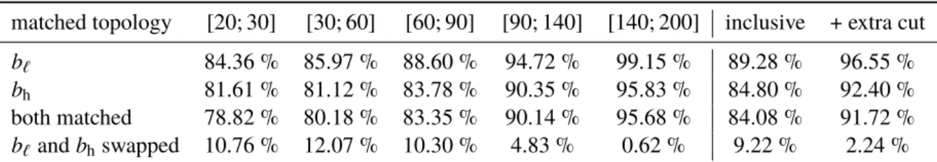
Figure3shows theb` λJVC distributions in the five pTbins of the analysis, divided by the simulated jet flavour.2 In dark blue is presented the distribution for simulated ¯b-jets identified as having a positive charge by the jet-lepton correlation (“ ¯bpos” in the legend), whereas the light blue distribution represent the events for which the simulated ¯b-jet is identified as having a negative charge (“ ¯bneg”). The dark (light) red histogram represents theλJVC distribution for simulatedb-jets identified as having a negative (positive) charge, “bneg” (“bpos”) in the legend. The contribution ofc-jets (yellow) and light-jets (green) is negligible in all but the firstb` pT bin. The uncertainty band correspond to the sum in quadrature of the statistical and systematic uncertainties, with the exception of the KLFitter systematic. The systematic uncertainty band comprises only shape effects, with acceptance effects removed by using the procedure described in Section7.
Figure4shows the final λJVC distribution after the unfolding step and mirroring the negatively charged b` candidates. The data/MC ratio in the bottom panel shows a good, but not perfect modelling of data offered by the simulation. Therefore this ratio is considered as data-to-simulation SF, which can be used to correctλJVCdistributions in simulated samples in physics analyses exploiting this observable.
In order to display more clearly the SF, the bottom panel is also presented separately in Figure5. The systematic uncertainty band in both Figures 4 and 5 comprises only shape effects, but includes the uncertainty associated to KLFitter.
2Jet flavour, in this context, has a broader meaning compared to the definition given in Section4, as it not only refers to b-/c-/light-jets, due to the further categorisation of theb-jets done according to the charge of the hadron that is used to label the flavour of the jet.
Events/bin
500 1000 1500 2000 2500 3000 3500
4000 Data b neg
b pos b neg pos
b c-jets
light-jets Total unc.
ATLAS Preliminary
= 13 TeV, 36.1 fb-1 s
30 GeV
T≤
≤ p 20
λJVC
blep
−2.5 −2−1.5 −1−0.5 0 0.5 1 1.5 2 2.5
Data/MC
0.75 0.875 1 1.125 1.25
(a)
Events/bin
2000 4000 6000 8000 10000 12000 14000 16000
18000 Data b neg
b pos b neg pos
b c-jets
light-jets Total unc.
ATLAS Preliminary
= 13 TeV, 36.1 fb-1 s
60 GeV
T≤
≤ p 30
λJVC
blep
−2.5 −2−1.5 −1−0.5 0 0.5 1 1.5 2 2.5
Data/MC
0.75 0.875 1 1.125 1.25
(b)
Events/bin
2000 4000 6000 8000 10000 12000
14000 Data b neg
b pos b neg pos
b c-jets
light-jets Total unc.
ATLAS Preliminary
= 13 TeV, 36.1 fb-1 s
90 GeV
T≤
≤ p 60
λJVC
blep
−2.5 −2−1.5 −1−0.5 0 0.5 1 1.5 2 2.5
Data/MC
0.75 0.875 1 1.125 1.25
(c)
Events/bin
1000 2000 3000 4000 5000 6000 7000 8000
9000 Data b neg
b pos b neg pos
b c-jets
light-jets Total unc.
ATLAS Preliminary
= 13 TeV, 36.1 fb-1 s
140 GeV
T≤
≤ p 90
λJVC
blep
−2.5 −2−1.5 −1−0.5 0 0.5 1 1.5 2 2.5
Data/MC
0.75 0.875 1 1.125 1.25
(d)
Events/bin
500 1000 1500 2000 2500
Data b neg
b pos b neg pos
b c-jets
light-jets Total unc.
ATLAS Preliminary
= 13 TeV, 36.1 fb-1 s
200 GeV
T≤
≤ p 140
λJVC
blep
−2.5−2 −1.5 −1 −0.5 0 0.5 1 1.5 2 2.5
Data/MC
0.75 0.875 1 1.125 1.25
(e)
Figure 3: λJVC distribution split into the different flavour components for the 5 pT bins of the analysis. (a) 20≤pT≤30 GeV (b) 30≤pT≤60 GeV (c) 60≤pT≤90 GeV (d) 90≤pT≤140 GeV (e) 140≤pT≥200 GeV.
Events/bin
500 1000 1500 2000 2500 3000 3500 4000 4500
Unfolded data b Unfolded b + Total unc.
ATLAS Preliminary
= 13 TeV, 36.1 fb-1 s
30 GeV
T≤
≤ p 20
lep) b * sgn(
λJVC
blep
−2.5 −2−1.5 −1−0.5 0 0.5 1 1.5 2 2.5
SF
0.75 0.875 1 1.125 1.25
(a)
Events/bin
2000 4000 6000 8000 10000 12000 14000 16000 18000 20000 22000
Unfolded data b Unfolded b + Total unc.
ATLAS Preliminary
= 13 TeV, 36.1 fb-1 s
60 GeV
T≤
≤ p 30
lep) b * sgn(
λJVC
blep
−2.5 −2−1.5 −1−0.5 0 0.5 1 1.5 2 2.5
SF
0.75 0.875 1 1.125 1.25
(b)
Events/bin
2000 4000 6000 8000 10000 12000 14000 16000
Unfolded data b Unfolded b + Total unc.
ATLAS Preliminary
= 13 TeV, 36.1 fb-1 s
90 GeV
T≤
≤ p 60
lep) b * sgn(
λJVC
blep
−2.5 −2−1.5 −1−0.5 0 0.5 1 1.5 2 2.5
SF
0.75 0.875 1 1.125 1.25
(c)
Events/bin
2000 4000 6000 8000
10000 Unfolded data
b Unfolded b + Total unc.
ATLAS Preliminary
= 13 TeV, 36.1 fb-1 s
140 GeV
T≤
≤ p 90
lep) b * sgn(
λJVC
blep
−2.5 −2−1.5 −1−0.5 0 0.5 1 1.5 2 2.5
SF
0.75 0.875 1 1.125 1.25
(d)
Events/bin
500 1000 1500 2000 2500
Unfolded data b Unfolded b + Total unc.
ATLAS Preliminary
= 13 TeV, 36.1 fb-1 s
200 GeV
T≤
≤ p 140
lep) b * sgn(
λJVC
blep
−2.5−2 −1.5 −1 −0.5 0 0.5 1 1.5 2 2.5
SF
0.75 0.875 1 1.125 1.25
(e)
Figure 4: FinalλJVCdistribution for theb` in the 5pTbins of the analysis. The distributions shown correspond to the sum of the unfoldedg(b)¯ and unfoldedg(b). The multiplication by sgn(b`) indicates that theg(b)distribution has been reflected about 0 for both data and simulation. (a) 20 ≤ pT ≤ 30 GeV (b) 30 ≤ pT ≤ 60 GeV (c)
≤ p ≤ ≤ p ≤ ≤ p ≤
λJVC
blep
−2.5 −2 −1.5 −1 −0.5 0 0.5 1 1.5 2 2.5
SF
0.6 0.8 1 1.2 1.4
ATLAS Preliminary
= 13 TeV, 36.1 fb-1
s
30 GeV T≤
≤ p 20
(a)
λJVC
blep
−2.5 −2 −1.5 −1 −0.5 0 0.5 1 1.5 2 2.5
SF
0.6 0.8 1 1.2 1.4
ATLAS Preliminary
= 13 TeV, 36.1 fb-1
s
60 GeV T≤
≤ p 30
(b)
λJVC
blep
−2.5 −2 −1.5 −1 −0.5 0 0.5 1 1.5 2 2.5
SF
0.6 0.8 1 1.2 1.4
ATLAS Preliminary
= 13 TeV, 36.1 fb-1
s
90 GeV T≤
≤ p 60
(c)
λJVC
blep
−2.5 −2 −1.5 −1 −0.5 0 0.5 1 1.5 2 2.5
SF
0.6 0.8 1 1.2 1.4
ATLAS Preliminary
= 13 TeV, 36.1 fb-1
s
140 GeV T≤
≤ p 90
(d)
λJVC
blep
−2.5 −2 −1.5 −1 −0.5 0 0.5 1 1.5 2 2.5
SF
0.6 0.8 1 1.2 1.4
ATLAS Preliminary
= 13 TeV, 36.1 fb-1
s
200 GeV T≤
≤ p 140
(e)
Figure 5: SF for theλJVCdistribution split into the different flavour components for the 5pTbins of the analysis. (a) 20≤pT≤30 GeV (b) 30≤pT≤60 GeV (c) 60≤pT≤90 GeV (d) 90≤pT≤140 GeV (e) 140≤pT≤200 GeV.
The uncertainty band corresponds to the statistical⊕systematic uncertainties, with the latter comprising only shape effects.
7 Systematic uncertainties
Many sources of systematic uncertainties can affect the derivation of the final SFs and will be discussed in the following sections. These include the detector related uncertainties as well as the modelling of the physical processes.
The effect of each uncertainty is evaluated by recomputing new SF using modified inputs that take into account the effect of the systematic uncertainty. Uncertainties affect both the acceptance and the shape of the samples. Thet¯t signal’s cross section uncertainty is not relevant for this analysis, given that the signal is re-weighted to reproduce the data, as described in Section5. More generally, acceptance effects are removed by normalising the modified templates so that their yields will match the total yield observed in data. For each systematic source, the envelope of the new SF around the nominal SF is taken as the uncertainty associated with the systematic source under consideration. All the systematic uncertainties are then summed in quadrature to obtain the final uncertainty on the result.
7.1 KLFitter uncertainty
The calibration analysis in this note relies heavily on the matching done by KLFitter; therefore, an assessment of the impact of its impurity is crucial. As mentioned in Section6, the KLFitter impurity is taken from the simulation. This does not allow for a straightforward method to estimate the associated uncertainty. Hence, a systematic uncertainty is needed in order to cover possible differences between the KLFitter purities in data and MC. It is derived by comparing the SF with the nominal selection of the analysis and a tightened selection intended to reduce the impurity further, so that by changing the purity it is possible to obtain an estimate of how much the result will change in different conditions.
The discriminating variable is the mass of the hadronic top candidate, reconstructed by swapping the two b-jets assignments. Its distribution is shown in Figure6. A peak is clearly visible at the position of the top mass for the wrongly matchedb-jets, indicating that swapping restores the correct matching between the b-jets and the top quark decays. Furthermore, the visible dip in the same mass range is a consequence of the KLFitter reconstruction: for events that are correctly matched by KLFitter, in the swapped assignment the candidate hadronic top quark mass is less likely to agree with the top quark mass. By rejecting events in the mass window between 120 GeV and 220 GeV, the KLFitter matching purity increases up to approximately 97%, as can be seen in Table1.
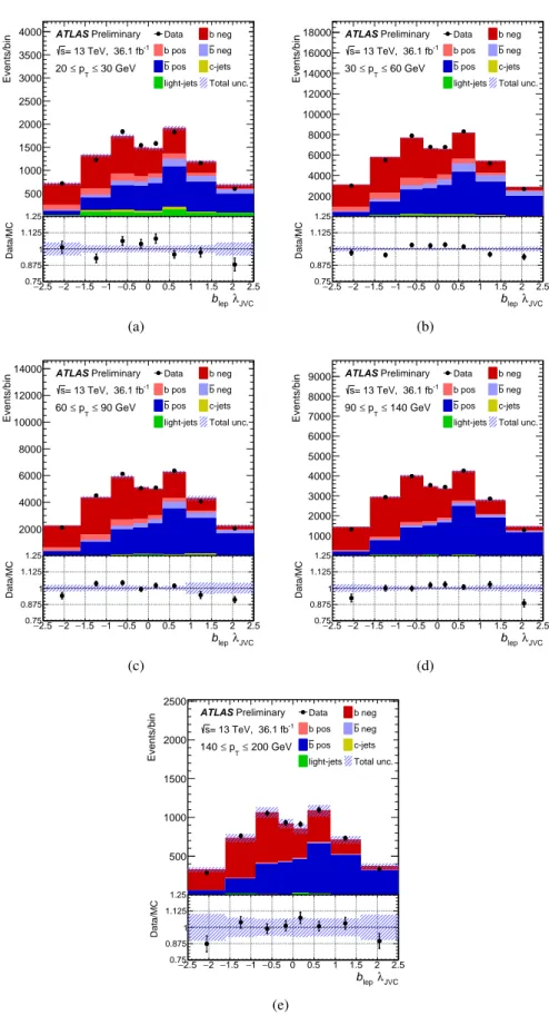
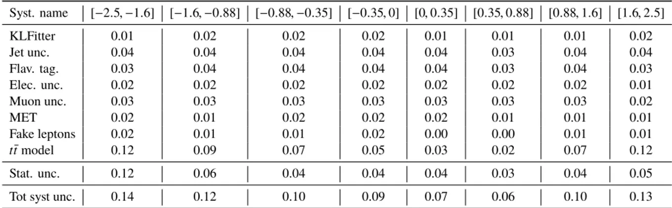
Figure 7shows the double ratio defined as the ratio of data/MC ratios with and without the additional criterion. Only the statistical uncertainty is shown and the correlation between the two subsamples it taken into account in its computation. The two selections provide compatible SF in most (but not all) of the bins; therefore the deviation of their double ratio from unity is taken as the relative uncertainty associated with the KLFitter impurity.
7.2 Luminosity
The uncertainty in the combined 2015+2016 integrated luminosity is 2.1%. It is derived following a methodology similar to that detailed in Ref. [58], from a calibration of the luminosity scale using x–y beam-separation scans performed in August 2015 and May 2016.
[GeV]
swap bhad
M
100 150 200 250 300 350 400 450
Events/5.00
0 1000 2000 3000 4000 5000
Bkg subtracted data
truth matched t
t
not truth matched t
t
ATLAS Preliminary
= 13 TeV, 36.1 fb-1
s
Figure 6: Mass of the top quark decaying hadronically, reconstructed by swapping the b` and the bh. The red histogram (“tt¯truth matched”) represents events for which the identification of theb`by KLFitter correctly matches the corresponding simulatedb` jet, whereas the blue histogram (“tt¯non truth matched”) collects all the remaining events. A peak at the value of the top quark mass is visible for the wrongly matched events. Events falling in the mass range identified by the dashed vertical lines at 120 GeVand 220 GeVare rejected in order to estimate the systematic uncertainty associated to KLFitter.
7.3 Object reconstruction 7.3.1 Jets
Uncertainties associated with jets arise from the efficiency of the pileup-jet rejection based on the JVT variable, as well as the jet energy scale (JES) and jet energy resolution (JER).
JES and its uncertainty were derived by combining information from test-beam data, LHC collision data and simulation [49]. The jet energy scale uncertainties are factorised into eight independent contributions.
Additional uncertainties related to the jet flavour, pileup treatment, η interpolation and extrapolation at highpTare considered as well, for a total of 21 independent sources. The JES uncertainty is about 5.5%
for jets withpT= 25 GeV and quickly decreasing with increasing jetpT, going below 1.5% for central jets withpT in the range of 100 GeV-1.5 TeV.
7.3.2 Flavour tagging
Flavour tagging efficiencies in simulated samples are corrected to match efficiencies measured in data.
Correction scale factors are derived for jets originating fromb-,c- and light-quarks separately in dedicated calibration analyses based ont¯t samples for the first two flavours, while for light-jets they are derived in multi-jet events using jets containing secondary vertices and tracks with impact parameters consistent with a negative lifetime [57].
λJVC
blep
−2.5 −2 −1.5 −1 −0.5 0 0.5 1 1.5 2 2.5
Ratio of selections
0.85 0.9 0.95 1 1.05 1.1 1.15 1.2 1.25 1.3 1.35
ATLAS Preliminary
= 13 TeV, 36.1 fb-1
s
30 GeV
T≤
≤ p 20
(a)
λJVC
blep
−2.5 −2 −1.5 −1 −0.5 0 0.5 1 1.5 2 2.5
Ratio of selections
0.85 0.9 0.95 1 1.05 1.1 1.15 1.2 1.25 1.3 1.35
ATLAS Preliminary
= 13 TeV, 36.1 fb-1
s
60 GeV
T≤
≤ p 30
(b)
λJVC
blep
−2.5 −2 −1.5 −1 −0.5 0 0.5 1 1.5 2 2.5
Ratio of selections
0.85 0.9 0.95 1 1.05 1.1 1.15 1.2 1.25 1.3 1.35
ATLAS Preliminary
= 13 TeV, 36.1 fb-1
s
90 GeV
T≤
≤ p 60
(c)
λJVC
blep
−2.5 −2 −1.5 −1 −0.5 0 0.5 1 1.5 2 2.5
Ratio of selections
0.85 0.9 0.95 1 1.05 1.1 1.15 1.2 1.25 1.3 1.35
ATLAS Preliminary
= 13 TeV, 36.1 fb-1
s
140 GeV
T≤
≤ p 90
(d)
λJVC
blep
−2.5 −2 −1.5 −1 −0.5 0 0.5 1 1.5 2 2.5
Ratio of selections
0.85 0.9 0.95 1 1.05 1.1 1.15 1.2 1.25 1.3 1.35
ATLAS Preliminary
= 13 TeV, 36.1 fb-1
s
200 GeV
T≤
≤ p 140
(e)
Figure 7: Double ratio of the SF obtained with the two selections for the fivepT bins of the analysis. Only the statistical error on the double ratio is shown and the correlation between the two subsamples is taken into account.
These uncertainties are estimated by varying each source of uncertainty up and down by one standard deviation and then the corresponding uncertainties are used as input into an eigenvector variation (EV) model with a reduction scheme such that only substantial EVs are treated separately while all small variations are combined together. A total of 6, 4 and 16 independent eigenvectors are considered forb,c and light-jets respectively.
An additional uncertainty is included due to the extrapolation of SFs for jets withpTbeyond the kinematic range used in each calibration analysis. Lastly, jets from hadronic τ lepton decays are considered as c-jets for the mis-tag rate corrections and systematic uncertainties. An additional source of systematic uncertainty is considered on the extrapolation betweenc-jets and theseτ-jets.
7.3.3 Leptons
Systematic uncertainties associated with leptons arise from the trigger, reconstruction, identification and isolation, as well as the lepton momentum scale and resolution. The corresponding efficiencies differ from data and simulation, therefore scale factors were provided to correct for these differences.
Efficiency SFs are derived using tag-and-probe techniques onZ →`+`−samples. The total uncertainty on efficiency SFs is < 0.5% for muons across the entire pT spectrum [46] and for electrons with pT >
30 GeV, while it exceeds 1% for lowpTelectrons [45].
Lepton momentum scale and resolution corrections are measured using reconstructed distributions of Z →`+`−, J/ψ →`+`−as well asW →eνevents.
7.3.4 Missing transverse energy
The uncertainties associated with the leptons, jet energy scales and resolutions, which are propagated to the final missing transverse momentum, are included under the corresponding per-object uncertainty category. There are three dedicated sources of uncertainties which are included, two resolution and one scale uncertainty on the soft track terms.
7.4 Pileup reweighting
A variation in the pileup reweighting of MC events is included to cover the uncertainty in the ratio of the predicted and measured inelastic cross-sections in the fiducial volume defined by MX > 13 GeV, where MX is the mass of the hadronic system [59].
7.5 tt¯modelling
Thet¯tsample is the most important one for this analysis, hence a few dedicated systematics are employed in order to cover possible mismodellings. These uncertainties are estimated by replacing the nominal MC sample with the alternative ones described in Section3.1.
In order to assess the uncertainty due to the MC generator choice, the Powheg+Pythia8 sample is compared to the sample generated with aMC@NLO interfaced with Pythia8.