ATLAS-CONF-2013-087 13August2013
ATLAS NOTE
ATLAS-CONF-2013-087
August 11, 2013
Performance and Validation of Q-jets at the ATLAS Detector in pp Collisions at √
s = 8 TeV in 2012
The ATLAS Collaboration
Abstract
The Q-jets technique introduces the idea of interpreting jets through multiple sets of possible showering histories. This approach allows jet observables, such as the jet mass, to be evaluated not simply as single values, but rather as distributions. The resulting dis- tributions can be interpreted statistically to form new observables, allowing the separation of boosted, hadronically-decaying particles from light quark and gluon backgrounds. We present a study of Q-jets in boosted, hadronically-decaying
Wboson and dijet samples, demonstrating the discriminating power of this technique. Different Q-jet parameters and observables are studied, and an optimal configuration based on physics performance and computational efficiency is proposed, leading to a factor of 15 in dijet rejection at a 50%
efficiency for jets from boosted, hadronically decaying
Wbosons. The impact of pile-up on the performance of this method is tested up to an average of 40 additional interactions per event and found to be weak. A performance comparison between the Q-jets algorithm and
N-subjettiness, a previously measured substructure observable which determines thecompatibility of a jet with the
N-subjet hypothesis, is presented.c
Copyright 2013 CERN for the benefit of the ATLAS Collaboration.
Reproduction of this article or parts of it is allowed as specified in the CC-BY-3.0 license.
1 Introduction
1.1 Overview
Sequential recombination clustering algorithms, such as the k
t-family [1] used by the ATLAS experiment, combine energy deposits in the calorimeter, assumed to result from quark and gluon fragmentation, into jets. The clustering history of the jet is the ordered set of combinations of particle momenta (2
→1 mergings) which produce the final jet four-vector. These clusterings can be thought of as mirroring the series of tree-like 1
→2 splittings in the parton shower which make up the jet. However, the parton shower is non-invertible, in the sense that there are many possible intermediate showering trees, not just a single unique one with a fixed set of conditions, which produce a given set of final state particles.
Jet clustering algorithms attempt to find an approximation to this inverse, leading back to the initial conditions, namely the colored particle(s) which initiated the jet.
The technique of Q-jets [2] acknowledges the non-uniqueness of the showering history by introduc- ing the idea of multiple clustering histories for jets. An initial jet, clustered using a standard recombi- nation algorithm such as anti-k
t[3], can be reclustered many times using an alternative set of clustering choices. Each set of choices (clustering history) creates a unique observable, whose distribution can be analysed for each final jet. There is no single correct clustering history, but rather a set of histories, which mimics the set of possible parton showers which initiated the jet. The resulting distributions can be used to generate observables allowing discrimination between massive, boosted objects and backgrounds from light quarks and gluons and in turn improve the statistical power of searches.
This note describes several studies performed to test the Q-jets algorithm in the context of boosted, hadronic W-jet tagging and is outlined in the following: Section
1.2gives a brief review of jet clustering and pruning algorithms in general and describes the Q-jets algorithm; the experimental setup as well as the data and Monte Carlo (MC) samples used in this study are presented in Sections
2and
3; Section4lists the selection criteria for the reconstructed physics objects and the events; the performance of Q-jets in fully reconstructed, simulated events as well as in data is reported in Section
5.1.2 The Q-jets algorithm
The distance parameters of two particles i and j is defined as d
i j=min
p
βTi,p
βTj ∆R
2i jR
2(1a)
d
iB=p
2Ti(1b)
where d
i jand d
iBare the inter-particle and jet-beam distance parameters respectively,
∆R
2i j =(y
i − yj)
2 +(φ
i −φj)
2and R is the jet radius parameter. The parameter
βdefines the clustering behavior of the specific clustering algorithm, the most common ones being
β =2 for the k
talgorithm,
β =0 for Cambridge/Aachen (C/A) [4,
5], and β = −2 for anti-kt. The form of the distance metric d
i jthus determines the order in which constituents are merged to form jets.
Traditional, k
t-family jet clustering proceeds according to the following algorithm [3,
6]:1. Calculate all d
i jand d
iBaccording to Equations
1aand
1b.2. Find the minimum of the set of d
i jand d
iB.
3. If the minimum is d
i j, combine i and j into a new constituent p and continue.
4. If the minimum is d
iB, define i a final, accepted jet, remove it from the list and continue.
5. Continue until no particles remain.
Further modifications of the jet are possible using jet grooming algorithms to achieve potential im- proved robustness against pile-up, mass resolution, etc. [7–10]. Pruning is an example of such an algo- rithm and proceeds as in the following [9]:
1. Start with a jet found by any jet algorithm and collect its constituents into a list. In this study, R
=0.7 anti-k
tjets are used.
2. Re-run a jet algorithm
1on the list of constituents, checking for the following conditions in each (i, j)
→p recombination;
z
i j=min(p
T,i,p
T,j)
|
p
~T,i+p
~T,j| <z
cutand
∆R
i j >d
cut.(2) 3. If both the conditions in the previous step are met, discard the softer of the two branches i or j
from the jet.
4. The resulting jet is the pruned jet, and can be compared with the jet found in step 1.
The jet pruning algorithm has been extensively studied by both the ATLAS and CMS collaborations and shown in some instances to improve the sensitivity of searches as compared to ungroomed jets [11–15].
The Q-jets algorithm, as used in this note, is a modification of the pruning algorithm. In principle the changed weights and clustering order provided by the Q-jets procedure can be generalized to other grooming algorithms, and indeed can replace the d
i jof Equation
1ain the general k
trecombination scheme. However, the largest effect is likely to be seen in jet pruning because of the merge-by-merge rejection defined in Equation
2, which has a higher probability of failure when well separated elementsare chosen to be merged by the Q-jets algorithm. The main difference lies in the distance metric used to determine the order of merging. The algorithm proceeds as follows:
1. Start with a jet found by any jet algorithm and collect the constituents into a list.
2. Compute a set of weights
ωi j, which reflect how likely a pair of four-vectors is to be merged, for all pairs of four-vectors. Here, the weights are chosen to be defined as:
ω(α)i j =
exp
−α
d
i j−d
mind
min
(3)
where
αis the rigidity which controls the sensitivity of the pair selection to the random number generation, d
i j≡∆R
2i j = ∆y2i j+ ∆φ2i jthe distance measure for the (i, j) pair and d
minthe minimum of the distance between all pairs. Then the probability
Ωi j=ωi j/Nis defined, where N
=Pωi j. 3. Instead of finding the single minimum d
i jas in Equation
1, generate a random number, usingEquation
3as a probability density function, and choose a pair of four-vectors as above according to the probabilities
Ωi j.
4. Consider this pair for merging, and veto (as in normal pruning) if they fail the cuts in Equation
2.5. Continue until all pairs are merged: the result is one Q-jet. The algorithm can be repeated multiple times to generate a distribution of Q-jets for every jet.
1Possible algorithms arektand C/A to ensure a meaningful clustering history.
By definition, the closest pair will have a weight
ωi j =1, while all others will have some weight that is suppressed by both the distance metric and the parameter
α. Asα → ∞, the behavior becomesequivalent to that of the standard pruning procedure. As
α →0, all pairs begin to acquire similar weights, and so the selected pair can very often be different from the closest pair. Therefore, unlike in both standard recombination techniques and jet pruning, re-running the Q-jets algorithm on a jet does not guarantee the same result, and indeed, it is precisely this behavior which allows the generation of distributions of Q-jets for every input jet.
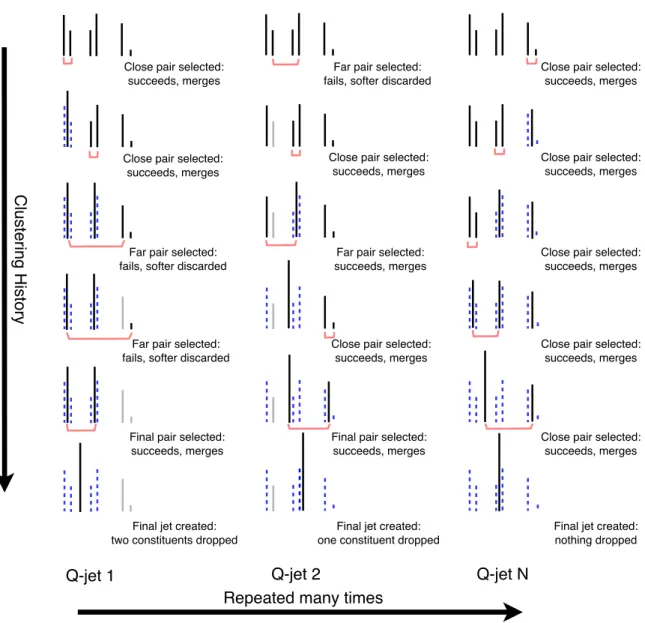
Figure
1diagrammatically demonstrates the Q-jets algorithm. The constituents of a single jet are reclustered many times using the algorithm, as shown in the different columns in the diagram. The final jet, at the end of each iteration, is slightly different because different constituents were discarded in the course of the clustering, and so each final jet has di
fferent kinematics, e.g. a di
fferent mass.
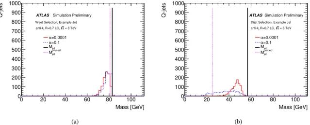
Figure
2shows typical examples of the mass distributions of Q-jets for several values of
αin simu- lation for a single jet from a dijet sample and a jet from a W boson decay in a t¯ t event. It is clear that the distributions have di
fferent shapes, with the distribution from light quark and gluon jets being generally wider. Further details on the selection criteria can be found in Section
4. The number of Q-jets generatedper jet, N
QJets, is a free parameter and was set to 1000 in this example. The z
cutand d
cutvalues used are 0.1 and m
jet/p
T,jet, respectively.
2 The ATLAS Detector and Data Sample
The ATLAS detector [16] is a multipurpose particle physics apparatus designed for proton-proton col- lisions in a high-luminosity environment at the LHC. It has a forward-backward symmetric cylindrical structure with nearly complete hermetic coverage. It comprises a precision tracking system at the inner- most part, highly segmented electromagnetic and hadronic calorimeters and a large muon spectrometer.
The inner detector (ID) covers the region
|η|<2.5
2and is composed of silicon pixel and microstrip de- tectors and a transition radiation tracker using drift tubes. The ID is surrounded by a 2 T superconducting solenoidal magnet. The electromagnetic calorimeter is located outside the solenoid and covers the range up to
|η|<3.2. It uses Liquid Argon (LAr) as active detector material and lead plates as passive absorber.
A scintillating tile sampling calorimeter within
|η|<1.7 and a LAr calorimeter between 1.5
< |η| <4.9 are used for hadronic and forward energy measurements. The ID and calorimeters are surrounded by a muon spectrometer (MS), which is composed of gas-filled precision tracking chambers up to
|η| <2.7 and trigger chambers up to
|η|<2.4. A toroidal magnetic field is generated by large barrel and end-cap air core magnets.
The full dataset used in the analyses presented in this note corresponds to (20.3
±0.6) fb
−1of inte- grated luminosity [17] collected at a centre of mass energy of
√s
=8 TeV and taken during periods in which the detector was fully operational. The ATLAS data quality criteria reject data with significant contamination from detector noise or issues in the read-out. These criteria are established separately for the barrel, endcap and forward regions, and differ depending on the trigger conditions and the type of physics object being reconstructed, such as jets, electrons, muons. The primary systems of interest in these studies are the electromagnetic and hadronic calorimeters.
A three-level trigger system is used to select interesting events. The Level 1 trigger is implemented in hardware and uses a subset of detector information to reduce the event rate to the design value of at most 75 kHz. This is followed by two software-based triggers, Level 2 and the Event Filter, which together
2ATLAS uses a right-handed coordinate system with its origin at the nominal interaction point (IP) in the centre of the detector, and the z-axis along the beam line. Thex-axis points from the IP to the centre of the LHC ring, and they-axis points upwards. Cylindrical coordinates (r,φ) are used in the transverse plane,φbeing the azimuthal angle around the beam line. Pseudorapidity is defined asη=−ln[tan(θ/2)] with the polar angleθ. Transverse momentum and energy are defined as pT=psinθandET=Esinθ, respectively.
Clustering History
Q-jet 1 Q-jet 2 Q-jet N
Far pair selected:
fails, softer discarded
Close pair selected:
succeeds, merges
Far pair selected:
succeeds, merges
Close pair selected:
succeeds, merges
Final pair selected:
succeeds, merges
Final jet created:
one constituent dropped
Repeated many times
Close pair selected:
succeeds, merges
Close pair selected:
succeeds, merges
Far pair selected:
fails, softer discarded
Far pair selected:
fails, softer discarded
Final pair selected:
succeeds, merges
Final jet created:
two constituents dropped
Close pair selected:
succeeds, merges
Close pair selected:
succeeds, merges
Close pair selected:
succeeds, merges
Close pair selected:
succeeds, merges
Close pair selected:
succeeds, merges
Final jet created:
nothing dropped
Figure 1: Diagrammatic example of several di
fferent iterations of the Q-jets algorithm in a simplified one-
dimensional space. Lines indicate jet constituents
/pseudo-jets, distances between lines indicate spatial
(∆ R) distances, and line heights indicate constituent energy. The same jet is reclustered many times, with
the clustering history starting at the top and proceeding downwards. At each step of the clustering, a
di
fferent pair is randomly selected, as described in the text, and the pruning criteria are checked: in the
case of a failure, the softer of the pair is discarded. Different iterations of the algorithm are displayed
in different columns. Discarded constituents are displayed in light grey; merged constituents in hashed
blue.
Mass [GeV]
0 20 40 60 80 100
Q-jets
0 100 200 300 400 500 600 700 800 900 1000
=0.0001 α
=0.1 α Mjet
pruned
Mjet
W-jet Selection, Example Jet = 8 TeV s R=0.7 LC, anti-kt
ATLAS Simulation Preliminary
(a)
Mass [GeV]
0 20 40 60 80 100
Q-jets
0 100 200 300 400 500 600 700 800 900 1000
=0.0001 α
=0.1 α Mjet
pruned
Mjet
Dijet Selection, Example Jet = 8 TeV s R=0.7 LC, anti-kt
ATLASSimulation Preliminary
(b)
Figure 2: Q-jet mass distribution when generating 1000 Q-jets per jet for (a) a jet from a W boson decay in a t¯ t event and for (b) a jet from a dijet event, reconstructed from topological clusters. The distribution for
α=100 is not shown as it coincides with the pruned jet mass, as expected.
reduce the event rate to a few hundred Hz.
To reject non-collision backgrounds, events are required to contain a primary vertex consistent with the LHC beam spot, reconstructed from at least 2 tracks each with transverse momentum p
trackT >400 MeV. All jets in the event built with the anti-k
talgorithm with R
=0.4 and a measured p
jetT >20 GeV are required to satisfy the “looser jet” requirements discussed in detail in Ref. [18]. These selections are designed to provide an efficiency to retain good quality jets of greater than 99.8% with as high a fake jet rejection as possible. In particular, this selection is very e
fficient in rejecting fake jets that arise due to calorimeter noise.
Two different data samples are used for this analysis. The first sample is selected by the primary single muon trigger chain, which is a logical OR of a p
T >24 GeV threshold, isolated muon trigger chain and a p
T >36 GeV threshold muon trigger chain without the isolation requirement. The second sample is selected by a single jet trigger chain with a p
T >145 GeV threshold for anti-k
tR
=0.4 jets.
This trigger is used to select events where the trigger jet p
Tis not too dissimilar from the p
Tregion of interest: however, this low threshold in p
Tleads to a very large trigger rate, and therefore only a small, randomly selected subset of the triggered events are recorded. The luminosity of the dijet data sample is thereby reduced to 36.3
±0.1 pb
−1, which still constitutes a sample large enough for the study.
3 Simulated Data Samples
Jets from hadronically decaying W bosons are selected from a t¯ t sample produced with the P
owheg[19,
20] generator, which incorporates next-to-leading order (NLO) QCD matrix elements into a partonshower framework through the Pythia 6 [21] generator. The parton distribution function (PDF) set used
is the leading order (LO) CTEQ6L1 [22]. The cross section is normalised to the approximate next-to-
next-to-leading order (NNLO) value [23]. The production of W and Z bosons in association with jets,
from both light and heavy flavor quarks, is simulated using the Alpgen [24] generator and the CTEQ6L1
PDF set. The parton shower and hadronization are modelled with P
ythia6. Diboson backgrounds are
simulated at LO with H
erwig[25] and scaled to NLO whereas single top production is modelled using
the MC@NLO [26] generator for the hard emission, Herwig for the parton shower and Jimmy for the
underlying event. Light quark and gluon jet background is modelled with dijet samples produced with
the P
ythia8 [27] generator. The ATLAS AU2 underlying event tune [28] and the CT10 [29] PDF set are used.
Pile-up, which is additional pp collisions apart from the primary hard collision in an event, is sim- ulated by overlaying additional unbiased pp collisions, which are generated with P
ythia8. These extra events are overlaid onto the hard scattering events according to the measured distribution of the average number
hµiof pp interactions per bunch crossing. The simulated proton bunches are organised in four trains of 36 bunches with a 50 ns spacing between the bunches. Therefore, the simulation also contains e
ffects from out-of-time pile-up, i.e. contributions from the collision of neighbouring bunches to that where the event of interest occurred. Simulated events are reweighted such that the MC distribution of
hµiagrees with the data. The present dataset has
µvalues ranging between 6 and 40 with a mean of 20.
The generated events are passed through the full G
eant4 [30] detector simulation [31] and subse- quently processed using the same reconstruction software as for data. Following this, the same trigger, event, quality, jet, and track selection criteria are applied to the MC simulation as are applied to the data. Corrections derived from the comparison of selection e
fficiencies measured in data and in MC are applied to the simulated events to reflect the performance observed in the data, including corrections to reproduce the muon momentum scale and resolution as well as the b-tagging performance observed in data.
4 Object and Event Selection
4.1 Object selection
Muon candidates are reconstructed by combining ID and MS tracks. The muon tracks are required to have a transverse momentum p
T >25 GeV,
|η| <2.5 and at least one hit in the silicon pixel detector, including one hit in the innermost layer, and at least four hits in the microstrip detectors. The muon candidate must satisfy track and calorimeter isolation as well as longitudinal impact parameter require- ments [32].
Jets are reconstructed from energy deposits in the calorimeters, grouped into topological clusters [33,
34] and calibrated at the hadronic scale [35] using the anti-ktcombination algorithm [6] with a radius parameter of R
=0.4 or R
=0.7. R
=0.4 jets are used for event selection only, while the objects of study are the R
=0.7 jets. R
=0.4 jets are corrected for pileup using the jet areas technique [36], and calibrated to the truth-particle scale using constants derived from Monte Carlo and validated in data [37].
R
=0.4 jets with p
T >25 GeV and
|η| <2.5
3are considered. At least 50% of the total transverse momentum from tracks associated to the jet must come from tracks associated to the primary vertex.
Jets produced by b-quarks are additionally required to be b-tagged using the MV1 algorithm at the 70%
working point [38].
R
=0.7 jets are required to have
|η| <1.8 such that they are fully contained within the tracking volume. All of the R
=0.7 jets are pruned using the C/A jet reconstruction algorithm with parameters z
cut <0.1 and d
cut >m/p
T. No jet energy scale or pileup corrections are applied to these jets in this study.
Track jets are reconstructed using ID tracks instead of calorimeter clusters. These tracks must satisfy longitudinal and transverse impact parameter cuts with respect to the primary vertex, p
T >500 MeV,
|η|<
2.5 and have at least six hits in the silicon detectors, where known dead sensors are counted as hits if they are traversed by a track candidate. The tracks are further required to have a fit-χ
2per degree of freedom of less than three.
3The jets for event level selection are allowed to be more forward than the jets selected for object studies, which are required to be fully contained within the tracker volume.
4.2 Event selection
As a preselection, only events that satisfy certain quality criteria on the detector operating conditions are retained. The selection is then split into two categories to single out either jets from hadronically decaying W bosons or from light quarks and gluons.
W-jet selection
A sample enriched in boosted hadronically-decaying W bosons is chosen from events that have passed a selection for t¯ t
→WbWb events, where one W boson decays leptonically into a muon and a neutrino, and the other decays hadronically. Events with exactly zero good electron candidates and one good muon candidate, which has to be matched to a muon trigger object, are required. At least four good anti-k
tR
=0.4 jets need to be reconstructed in the event, out of which at least one is required to be b-tagged at the 70% operating point of the MV1 algorithm. The missing transverse energy E
missTin the event must be larger than 20 GeV and the sum of the E
missTand the transverse mass of the leptonically-decaying W boson, reconstructed by combining the muon candidate and the E
Tmiss, must be larger than 60 GeV. The highest p
Tanti-k
tR
=0.7 jet must have
|η| <1.8, to ensure that it is contained in the tracking volume.
The same jet must not overlap with a selected b-tagged jet and is required to have a pruned mass of 50
<m
prunedjet <110 GeV and 200
<p
T <350 GeV.
Dijets selection
After applying the preselection criteria, the second highest p
Tanti-k
tR
=0.7 jet is considered and required to have a pruned mass of 50
<m
prunedjet <110 GeV and 200
<p
T <350 GeV. The leading anti-k
tR
=0.4 jet is required to pass the single jet trigger described in section
2and have p
T >180 GeV in order to lie on the fully e
fficient region of the trigger turn-on curve. Furthermore, to reduce biases introduced by the trigger selection, the leading anti-k
tR
=0.4 jet is required to be isolated from the second highest p
Tanti-k
tR
=0.7 jet with
∆φ >2.0 to guarantee that no part of the jet which fired the trigger overlaps with the jet under study.
5 Jet Volatility
5.1 Overview
The main discriminating power of the Q-jets technique comes from exploiting the difference in widths of the Q-jets mass distributions for a given jet. The mass variation in dijets is expected to be larger than for heavy, boosted objects, because mass in dijet events typically originates from wide angle, soft radiation which is likely to be removed by the pruning and random ordering of the Q-jets algorithm. A variable that is deemed to be sensitive to the mass variation is called the volatility, and it is defined as
ν= Γ/hmi
(4)
where
Γ = phm2i − hmi2
and
hmiare the RMS deviation and the mean of the pruned jet mass distribu- tion, respectively.
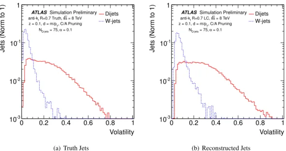
Figure
3shows the separation in the volatility between W-jets from the t¯ t sample and light quark and
gluon jets. The latter generally have a larger volatility as a result of large variations when running the
Q-jets algorithm whereas the former generally have a smaller volatility. This is understood as the origin
of their mass, the hadronic decay of a massive particle, is more resilient to the variations caused by the
Q-jets algorithm. Truth jets, which are constructed from truth particles taken from the MC event record
shown in Figure
3(a), have slightly lower volatility than jets reconstructed from topological clusters, asshown in Figure
3(b).Volatility
0 0.2 0.4 0.6 0.8 1
Jets (Norm to 1)
10-3
10-2
10-1
1
Dijets W-jets
= 8 TeV s R=0.7 Truth, anti-kt
, C/A Pruning z = 0.1, d = m/pT
= 0.1 = 75, α
Q-jets
N
ATLAS Simulation Preliminary
(a) Truth Jets
Volatility
0 0.2 0.4 0.6 0.8 1
Jets (Norm to 1)
10-3
10-2
10-1
1
Dijets W-jets
= 8 TeV s R=0.7 LC, anti-kt
, C/A Pruning z = 0.1, d = m/pT
= 0.1 = 75, α
Q-jets
N
ATLAS Simulation Preliminary
(b) Reconstructed Jets
Figure 3: The volatility distributions (log scale on
yaxis), for
α =0.1 and 75 Q-jets per jet, of W- jets compared to dijets for (a) truth-particle jets and for (b) jets reconstructed from locally calibrated topological clusters.
5.2 Optimization vs. α
As noted in Section
1, the volatility variable is expected to depend on the rigidity, α. In particular,as
α → ∞, the random element of Q-jets is lost, and the power of volatility decreases. Likewise, as
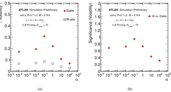
α →0, the weighting by the distance metric loses importance, and the selection of mergings becomes completely random and a reduction of separation is again expected. Figure
4shows the mean of the volatility distribution as well as the significance of the volatility as a function of
α. The significance isdefined as the ratio of the absolute difference of the mean W-jet selection and dijet selection volatilities to the sum in quadrature of the respective RMS values. It can be seen that the optimal separation occurs at
α=0.1. A full comparison of signal efficiency versus background rejection
4is presented in Section
5.6.5.3 Optimization of Q-jet number
Apart from the rigidity
α, another free parameter of the Q-jets algorithm isN
QJets, which is the number of Q-jets generated per jet to calculate the volatility. In principle,
νis defined for N
QJets→ ∞, but in practiceit must be estimated from finite samples. As N
QJetsincreases, the volatility is expected to become more robust against statistical fluctuations and therefore a stronger discriminant. However, the computation time grows significantly with increasing N
QJets, which can lead to a heavy load on computing resources.
Figure
5displays the mean volatility as a function of N
QJets. It shows that the separation between W-jets and dijets is fairly stable and suggests that analyses are able to use N
QJetsvalues a low as 25
−50 to observe similar performance to the results presented in this note, where N
QJets =75 is generally used.
Section
5.6presents a full signal e
fficiency versus background rejection optimization for this variable.
4The efficiency is defined as the ratio of the number of kept to rejectedW-jets whereas the rejection is defined as the ratio of the number of rejected to kept light quark and gluon jets.
α 10-510-4 10-3 10-2 10-1 1 10 102 103
〉 Volatility〈
0 0.1 0.2 0.3 0.4 0.5 0.6
ATLAS Simulation Preliminary = 8 TeV s R=0.7 LC, anti-kt
z = 0.1, d = m/pT
= 75
Q-jets
C/A Pruning, N
Dijets W-jets
(a)
α 10-5 10-4 10-3 10-2 10-1 1 10 102 103
Significance (Volatility)
0 0.2 0.4 0.6 0.8 1 1.2 1.4 1.6 1.8 2
ATLAS Simulation Preliminary = 8 TeV s R=0.7 LC, anti-kt
z = 0.1, d = m/pT
= 75
Q-jets
C/A Pruning, N
W vs. Dijets
(b)
Figure 4: Distributions of (a) the volatility for W-jets and dijets and (b) the significance of the volatility as a function of the rigidity
α. The optimal separation in mean and optimal significance is observed at α=0.1. The significance is defined as the ratio of the difference between the mean dijet and mean W-jet selection volatilities to the sum in quadrature of the respective RMS values.
Q-jets
N 10 20 30 40 50 60 70 80
〉 Volatility〈
0 0.1 0.2 0.3 0.4 0.5 0.6
ATLAS Simulation Preliminary = 8 TeV s R=0.7 LC, anti-kt
z = 0.1, d = m/pT
= 75
Q-jets
C/A Pruning, N
Dijets W-jets
(a)
Q-jets
N 10 20 30 40 50 60 70 80
Significance (Volatility)
0 0.2 0.4 0.6 0.8 1 1.2 1.4 1.6 1.8 2
ATLAS Simulation Preliminary = 8 TeV s R=0.7 LC, anti-kt
z = 0.1, d = m/pT
= 75
Q-jets
C/A Pruning, N
W vs. Dijets
(b)
Figure 5: Distributions of (a) the volatility for W-jets and dijets and (b) the significance of the volatility
as a function of N
QJets. The significance is defined as the ratio of the difference between the mean dijet
and mean W-jet selection volatilities to the sum in quadrature of the respective RMS values.
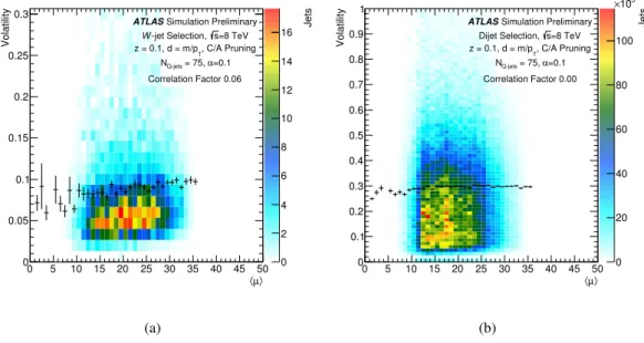
5.4 Performance versus pile-up
Volatility shows only a small dependence on the average number of interactions per bunch crossing, up to 40, for both W-jets and dijets, as shown in Figures
6(a)and
6(b)respectively. As jet pruning is designed partly to remove pileup from large R jets, volatility is likewise expected to have weak sensitivity to pileup, as observed [9,
39].Jets
0 2 4 6 8 10 12 14 16
〉 µ
〈 0 5 10 15 20 25 30 35 40 45 50
Volatility
0 0.05 0.1 0.15 0.2 0.25
0.3 ATLAS Simulation Preliminary
=8 TeV s -jet Selection, W
, C/A Pruning z = 0.1, d = m/pT
α=0.1 = 75,
Q-jets
N
Correlation Factor 0.06
(a)
Jets
0 20 40 60 80 100
103
×
〉 µ
〈 0 5 10 15 20 25 30 35 40 45 50
Volatility
0 0.1 0.2 0.3 0.4 0.5 0.6 0.7 0.8 0.9 1
Simulation Preliminary ATLAS
=8 TeV s Dijet Selection,
, C/A Pruning z = 0.1, d = m/pT
α=0.1 = 75,
Q-jets
N
Correlation Factor 0.00
(b)
Figure 6: Volatility as a function of the average number of interactions per bunch crossing for (a) W- jets and (b) dijets for jets reconstructed from topological clusters. The black points represent the mean volatility as a function of
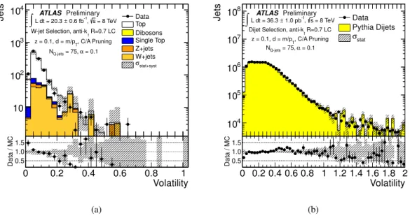
hµi.5.5 Data / MC agreement
The comparison of data to MC for the volatility variable is shown in Figure
7for an
αvalue of 0.1. Fair agreement is seen in all cases, although in the dijet sample it is generally better and stable over the full range of volatility. In the W-jet sample, the Monte Carlo predicts higher values of volatility than seen in data. The comparison of the pruned jet mass distribution in data and simulation in the W mass peak region between 50 GeV and 110 GeV is shown in Figure
8.Systematic uncertainties
The di
fferent sources of systematic uncertainties that are considered can be split into two main cate- gories: those a
ffecting the overall normalization and those a
ffecting the shape of the distributions and the acceptance. For the first category, a 5% uncertainty on the next-to-next-to-leading order in QCD and next-to-next-to-leading logarithmic order t¯ t cross-section [23] is applied as well as a 2.8% uncertainty on the integrated luminosity. The latter is derived, following the same methodology as that detailed in Ref. [40], from a preliminary calibration of the luminosity scale derived from beam-separation scans performed in November 2012. For the second category, the major sources of uncertainties considered are related to the jet energy scale (JES), jet energy resolution (JER), jet mass scale (JMS) and b-tagging efficiency. The systematic uncertainties from these different sources are combined and shown in the shaded band in Figures
7(a)and
8(a)together with the statistical uncertainty of the simulated samples.
Figures
7(b)and
8(b)show statistical uncertainties only.
Jets
10 102
103
104
= 8 TeV s
-1, 0.6 fb L dt = 20.3 ±
∫
R=0.7 LC W-jet Selection, anti-kt
, C/A Pruning z = 0.1, d = m/pT
= 0.1 α = 75,
Q-jets
N
ATLAS Preliminary Data Top Dibosons Single Top Z+jets W+jets
stat+syst
σ
Volatility
0 0.2 0.4 0.6 0.8 1
Data / MC0.5 1.0 1.5
(a)
Jets
104
105
106
107
108
= 8 TeV s
-1, 1.0 pb L dt = 36.3 ±
∫
R=0.7 LC Dijet Selection, anti-kt
, C/A Pruning z = 0.1, d = m/pT
= 0.1 α = 75,
Q-jets
N
ATLAS Preliminary
Data Pythia Dijets σstat
Volatility 0 0.2 0.4 0.6 0.8 1 1.2 1.4 1.6 1.8 2
Data / MC0.5 1.0 1.5
(b)
Figure 7: Volatility for reconstructed calorimeter jets in data and in simulation for (a) a W-jet selection and for (b) a dijet selection. W-jet selection plots show statistical and systematic uncertainties whereas dijet selection plots show statistical uncertainties only.
Jets
0 20 40 60 80 100 120 140
160
∫
L dt = 20.3 ± 0.6 fb-1, s = 8 TeV R=0.7 LC W-jet Selection, anti-kt, C/A Pruning z = 0.1, d = m / pT
ATLAS Preliminary Data Top Dibosons Single Top Z+jets W+jets
stat+syst
σ
Pruned Mass [GeV]
20 40 60 80 100 120
Data / MC0.5 1.0 1.5
(a)
Jets
0 1 2 3 4 5 6 7 8
106
×
= 8 TeV s
-1, 1.0 pb
± L dt = 36.3
∫
R=0.7 LC Dijet Selection, anti-kt
, C/A Pruning z = 0.1, d = m / pT
ATLAS Preliminary Data Pythia Dijets σstat
Pruned Mass [GeV]
20 40 60 80 100 120
Data / MC0.5 1.0 1.5
(b)
Figure 8: Pruned, leading jet mass distribution in data and in simulation for (a) a W-jet selection and
for (b) a dijet selection. W-jet selection plots show statistical and systematic uncertainties whereas dijet
selection plots show statistical uncertainties only.
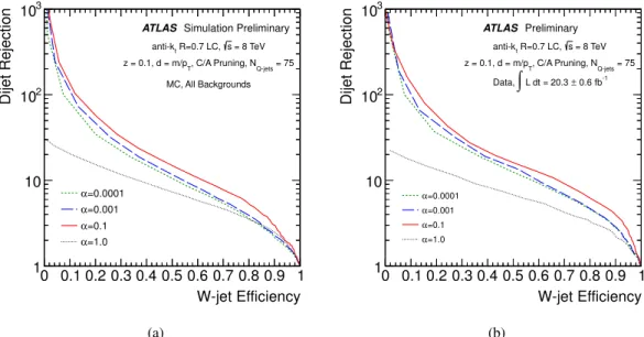
5.6 Signal e ffi ciency and background rejection
As enriched samples of W-jets and dijets are selected in both data and MC, the combined light quark and gluon jet rejection as a function of W-jet efficiency can be measured separately in both data and MC.
The W-jet efficiency and dijet rejection (the inverse of the dijet efficiency) are calculated by scanning cut values of the volatility distributions in Figure
7. The results in Figure9show that a rejection factor of 15 for a mixed sample of light quark and gluon jets can be obtained at a 50% W-jet efficiency working point, and they also confirm that
α=0.1 provides the optimal background rejection for a fixed signal efficiency as discussed in section
5.2. All samples are selected as described in sections4.1and
4.2. Figure9(a)shows the efficiency in MC and includes the backgrounds discussed in Section
3while Figure
9(b)shows the efficiency in data and confirms the rejection observed in MC.
W-jet Efficiency 0 0.1 0.2 0.3 0.4 0.5 0.6 0.7 0.8 0.9 1
Dijet Rejection
1 10 102
103
= 8 TeV s R=0.7 LC, anti-kt
= 75
Q-jets
, C/A Pruning, N z = 0.1, d = m/pT
MC, All Backgrounds ATLAS Simulation Preliminary
=0.0001 α
=0.001 α
=0.1 α
=1.0 α
(a)
W-jet Efficiency 0 0.1 0.2 0.3 0.4 0.5 0.6 0.7 0.8 0.9 1
Dijet Rejection
1 10 102
103
= 8 TeV s R=0.7 LC, anti-kt
= 75
Q-jets
, C/A Pruning, N z = 0.1, d = m/pT
0.6 fb-1
L dt = 20.3 ±
∫
Data,
ATLAS Preliminary
=0.0001 α
=0.001 α α=0.1 α=1.0
(b)
Figure 9: Signal e
fficiency versus background rejection in (a) signal MC with all backgrounds and in (b) data for several values of
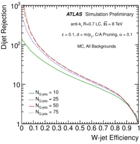
α.In Figure
10, the signal efficiency to background rejection is computed for several values of N
QJets. Values of N
QJets >25 show very similar results, suggesting that generation of as few as 25 Q-jets per jet can provide near optimal performance as discussed in section
5.3.5.7 Track jets performance
As a cross-check on the method, the studies are also performed using jets reconstructed from tracks in
the inner detector while event selections are still performed on the R
=0.4 calorimeter jets. As shown in
Figure
11(a), some discrimination betweenW-jets and dijets continues to exist for jets constructed from
tracks, but the separation is significantly reduced compared to the calorimeter variable. This is expected
due to the missing neutral content, which varies widely from jet to jet due to the fragmentation of an
individual jet, and consequently means that distributions for discriminating variables are generally less
well separated. Figure
11(b)shows the comparison of data and simulation as a function of volatility for
the W-jet selection.
W-jet Efficiency 0 0.1 0.2 0.3 0.4 0.5 0.6 0.7 0.8 0.9 1
Dijet Rejection
1 10 102
103
= 8 TeV s R=0.7 LC, anti-kt
= 0.1 , C/A Pruning, α z = 0.1, d = m/pT
MC, All Backgrounds ATLAS Simulation Preliminary
= 10
Q-jets
N = 25
Q-jets
N = 50
Q-jets
N = 75
Q-jets
N
Figure 10: Signal efficiency versus background rejection for several values of N
QJets. Performance stabilizes for N
QJets >25.
Volatility
0 0.2 0.4 0.6 0.8 1
Jets (Norm to 1)
10-3
10-2
10-1
1
Dijets W-jets
= 8 TeV s R=0.7 Track, anti-kt
, C/A Pruning z = 0.1, d = m/pT
= 0.1 = 75, α
Q-jets
N
ATLAS Simulation Preliminary
(a)
Jets
10 102
103
104
= 8 TeV s
-1, 0.6 fb
± L dt = 20.3
∫
R=0.7 Track W-jet Selection, anti-kt
, C/A Pruning z = 0.1, d = m/pT
= 0.1 = 75, α
Q-jets
N
ATLAS Preliminary Data Top Dibosons Single Top Z+jets W+jets
stat+syst
σ
Volatility
0 0.2 0.4 0.6 0.8 1
Data / MC0.5 1.0 1.5
(b)
Figure 11: Volatility, constructed using track-jets, of W-jets and dijets (a) and data/MC agreement for
the same in the W-jet selection (b). The separation is reduced compared to calculating the variable from
calorimeter clusters.
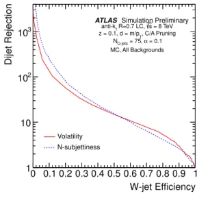
5.8 Q-jets versus N-subjettiness performance
To compare the volatility variable of the Q-jets algorithm to other substructure algorithms, the
τmin21N- subjettiness variable with one pass of the minimization algorithm on the k
taxes has been chosen
5[41–
43]. Figure12
shows that the performance of the two variables is comparable over a large range of signal e
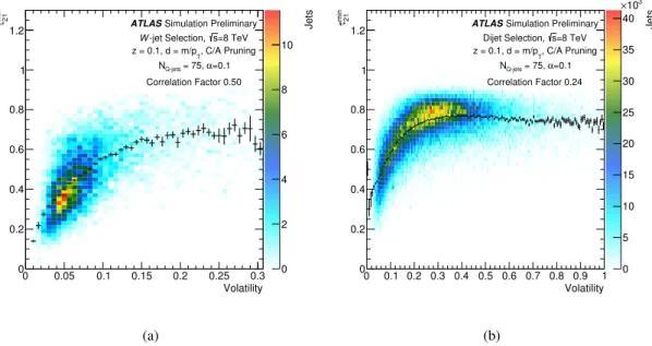
fficiency and background rejection values. Figure
13shows the correlations between the two variables with correlation factors of 50% and 24% for jets from a hadronically-decaying W boson and dijets respectively. In particular, for the dijet selection shown in Figure
13(b), the slope between thetwo variables is reduced for large volatility values. This confirms previous observations [44] that a combination of the two variables will give an improved performance.
W-jet Efficiency 0 0.1 0.2 0.3 0.4 0.5 0.6 0.7 0.8 0.9 1
Dijet Rejection
1 10 102
103 anti-kt R=0.7 LC, s = 8 TeV
, C/A Pruning z = 0.1, d = m/pT
= 0.1 = 75, α
Q-jets
N
MC, All Backgrounds ATLAS Simulation Preliminary
Volatility N-subjettiness
Figure 12: Signal efficiency versus background rejection for the volatility and
τmin21variables.
5Note that while the jet selections are performed using the pruned jet kinematics,N-subjettiness is calculated with the full jet constituents, consistent with the approach that has delivered best experimental performance in previous efforts [41].
Jets
0 2 4 6 8 10
Volatility
0 0.05 0.1 0.15 0.2 0.25 0.3
min 21τ
0 0.2 0.4 0.6 0.8 1
1.2 ATLAS Simulation Preliminary
=8 TeV s -jet Selection, W
, C/A Pruning z = 0.1, d = m/pT
=0.1 = 75, α
Q-jets
N
Correlation Factor 0.50
(a)
Jets
0 5 10 15 20 25 30 35 40 103
×
Volatility 0 0.1 0.2 0.3 0.4 0.5 0.6 0.7 0.8 0.9 1
min 21τ
0 0.2 0.4 0.6 0.8 1
1.2 ATLAS Simulation Preliminary
=8 TeV s Dijet Selection,
, C/A Pruning z = 0.1, d = m/pT
=0.1 = 75, α
Q-jets
N
Correlation Factor 0.24
(b)
Figure 13: Distributions of the
τmin21(N-subjettiness) and volatility (Q-jets) variables for (a) a W-jet selection and (b) a dijet selection. The black points represent the mean
τmin21value as a function of volatility.
6 Conclusions
The performance of the Q-jets reclustering algorithm and the resulting jet volatility distributions have been explored and this technique has been confirmed to discriminate between W-jets and light quark and gluon jets. Two free parameters of the algorithm have been studied and optimal values for the rigidity at
α =0.1 and for the number of Q-jets per jet of N
QJets >25 have been determined. No strong pile-up dependence is observed for the volatility variable, while the distribution for jets from a W boson decay are slightly more sensitive to additional interactions than light quark and gluon jets. The performance of the Q-jet algorithm in terms of discrimination power between W-jets and light quark and gluon jets has been studied for jets reconstructed from topological calorimeter clusters and for jets reconstructed from inner detector tracks; the discrimination of the latter is seen to be weaker. This degradation in performance is partially due to the fact that neutral hadrons do not leave tracks in the inner detector.
From these studies, the application of a volatility requirement is shown to give a factor of 15 in dijet rejection for 50% W-jet e
fficiency for jets with 200 GeV
<p
T <350 GeV. The separation is validated in-situ by comparing distributions of samples enriched in W-jets and light quark and gluon jets: very good agreement is observed in multijet events, and fairly good agreement is seen in W-jets.
The separation power of Q-jets is also tested directly in data using these samples, and the Monte Carlo predictions are confirmed. Lastly, the signal efficiency and background rejection of the volatility variable has been shown to be similar to the
τmin21N-subjettiness variable, while the former performs slightly better in the high W-jet e
fficiency region. The correlations between these two variables have been studied and interesting regions of decorrelaton are observed, particularly for the dijet selection. This suggests that a combination of the two variables could lead to an improved performance.
The strong performance of using volatility as a discriminating variable has motivated the investi- gation of its use in hadronically-decaying boosted object searches such as diboson and t¯ t resonances.
Further future plans include the use of Q-jet distributions as event weights, which has been shown in
theoretical studies to improve the statistical significance of searches [2,
45].References
[1] S. D. Ellis and D. E. Soper, Successive combination jet algorithm for hadron collisions, Phys.Rev.
D48
(1993) 3160–3166, arXiv:hep-ph/9305266 [hep-ph].
[2] S. D. Ellis et al., Qjets: A Non-Deterministic Approach to Tree-Based Jet Substructure, Phys.Rev.Lett.
108(2012) 182003, arXiv:1201.1914 [hep-ph].
[3] M. Cacciari, G. P. Salam, and G. Soyez, The anti-k
tjet clustering algorithm, JHEP
0804(2008) 063, arXiv:0802.1189 [hep-ph].
[4] Y. L. Dokshitzer, G. Leder, S. Moretti, and B. Webber, Better jet clustering algorithms, JHEP
9708(1997) 001, arXiv:hep-ph/9707323 [hep-ph].
[5] M. Wobisch and T. Wengler, Hadronization corrections to jet cross-sections in deep inelastic scattering, arXiv:hep-ph/9907280 [hep-ph].
[6] M. Cacciari, G. P. Salam, and G. Soyez, FastJet User Manual, Eur.Phys.J.
C72(2012) 1896, arXiv:1111.6097 [hep-ph].
[7] J. Thaler and L.-T. Wang,
Strategies to identify boosted tops, JHEP (July, 2008) 092,arXiv:0806.0023 [hep-ph].
[8] S. D. Ellis, C. K. Vermilion, and J. R. Walsh, Techniques for improved heavy particle searches with jet substructure, Phys. Rev.
D80(2009) 051501, arXiv:0903.5081 [hep-ph].
[9] S. D. Ellis, C. K. Vermilion, and J. R. Walsh, Recombination Algorithms and Jet Substructure:
Pruning as a Tool for Heavy Particle Searches, Phys. Rev.
D 81(2010) 094023, arXiv:0912.0033 [hep-ph].
[10] D. Krohn, J. Thaler, and L.-T. Wang, Jet trimming, JHEP
2010(2010) 20, arXiv:0912.1342 [hep-ph].
[11] ATLAS Collaboration, Performance of large-R jets and jet substructure reconstruction with the ATLAS detector, ATLAS-CONF-2011-065. http://cdsweb.cern.ch/record/1459530.
[12] ATLAS Collaboration, Studies of the impact and mitigation of pile-up on large radius and groomed jets in ATLAS at
√s
=7 TeV, ATLAS-CONF-2011-066.
http://cdsweb.cern.ch/record/1459531.
[13] ATLAS Collaboration, A search for t¯ t resonances in the lepton plus jets final state with ATLAS using 4.7 fb
−1of pp collisions at
√s
=7 TeV , arXiv:1305.2756 [hep-ex].
[14] CMS Collaboration, Search for heavy resonances in the W
/Z-tagged dijet mass spectrum in pp collisions at 7 TeV, Phys.Lett.
B723(2013) 280–301, arXiv:1212.1910 [hep-ex].
[15] ATLAS Collaboration, Performance of jet substructure techniques for large-R jets in proton-proton collisions at
√s
=7 TeV using the ATLAS detector, arXiv:1306.4945 [hep-ex].
[16] ATLAS Collaboration, The ATLAS Experiment at the CERN Large Hadron Collider, JINST
3(2008) S08003.
[17] ATLAS Collaboration, Luminosity Determination in pp Collisions at
√s
=7 TeV using the ATLAS
Detector in 2011, ATLAS-CONF-2011-116. https://cdsweb.cern.ch/record/1376384.
[18] ATLAS Collaboration, Selection of jets produced in proton-proton collisions with the ATLAS detector using 2011 data, ATLAS-CONF-2012-020.
https://cdsweb.cern.ch/record/1430034.
[19] P. Nason, A New method for combining NLO QCD with shower Monte Carlo algorithms, JHEP
0411(2004) 040, arXiv:hep-ph/0409146 [hep-ph].
[20] S. Frixione, P. Nason, and C. Oleari, Matching NLO QCD computations with Parton Shower simulations: the POWHEG method, JHEP
0711(2007) 070, arXiv:0709.2092 [hep-ph].
[21] T. Sjostrand, S. Mrenna, and P. Z. Skands, PYTHIA 6.4 physics and manual, JHEP
0605(2006) 026, arXiv:0603175 [hep-ph].
[22] P. M. Nadolsky et al., Implications of CTEQ global analysis for collider observables, Phys. Rev.
D 78(2008) 013004, arXiv:0802.0007 [hep-ph].
[23] M. Aliev et al., HATHOR: HAdronic Top and Heavy quarks crOss section calculatoR, Comput.Phys.Commun.
182(2011) 1034–1046, arXiv:1007.1327 [hep-ph].
[24] M. L. Mangano et al., ALPGEN, a generator for hard multiparton processes in hadronic collisions, JHEP
07(2003) 001, arXiv:0206293 [hep-ph].
[25] G. Corcella et al., HERWIG 6: an event generator for Hadron Emission Reactions With Interfering Gluons (including supersymmetric processes), JHEP
01(2001) 010, arXiv:hep-ph/0011363.
[26] S. Frixione and B. R. Webber, Matching NLO QCD computations and parton shower simulations, JHEP
06(2002) 029, arXiv:hep-ph/0204244.
[27] T. Sj¨ostrand, S. Mrenna, and P. Z. Skands, A Brief Introduction to PYTHIA 8.1, Comput. Phys.
Commun.
178(2008) 852–867, arXiv:0710.3820 [hep-ph].
[28] ATLAS Collaboration, Further ATLAS tunes for Pythia6 and Pythia8,
ATLAS-PHYS-PUB-2011-014. http://cdsweb.cern.ch/record/1400677.
[29] H.-L. Lai et al., New parton distributions for collider physics, Phys. Rev.
D82(2010) 074024, arXiv:1007.2241 [hep-ph].
[30] GEANT4 Collaboration, S. Agostinelli et al., GEANT4: A simulation toolkit, Nucl. Instrum. Meth.
A506