ATLAS-CONF-2012-066 04July2012
ATLAS NOTE
ATLAS-CONF-2012-066
June 26, 2012
Studies of the impact and mitigation of pile-up on large radius and groomed jets in ATLAS at √
s = 7 TeV
The ATLAS Collaboration
Abstract
Large radius jets provide one avenue towards e
fficient reconstruction of massive boosted objects whose decay products are sufficiently collimated so as to make standard reconstruc- tion techniques impractical. The potentially adverse impact of additional proton-proton in- teractions on such large jets is assessed for a variety of jet types and hadronic final state topologies. The mitigation of these effects via jet grooming algorithms such as trimming, pruning, and filtering is then studied for high transverse momentum jets at
√s =
7 TeV using an integrated luminosity of 4.7 fb
−1collected with the ATLAS detector. A total of 29 jet algorithms and grooming configuration combinations are studied. The application of jet trimming and filtering significantly improves the robustness of large-R jets and reduces their sensitivity to the intense environment of the high-luminosity LHC. The consequence is an overall improvement in the physics potential of searches for heavy boosted objects.
c
Copyright 2012 CERN for the benefit of the ATLAS Collaboration.
Reproduction of this article or parts of it is allowed as specified in the CC-BY-3.0 license.
1 Introduction
Jets have historically been utilized at high energy colliders as proxies for the quarks and gluons pro- duced in the primary hard interaction. The jet definition is the means by which the four-momenta of those partons, stable hadrons, or even experimentally measured calorimeter energy deposits are typically compared. Many studies in ATLAS have demonstrated the performance [1] and physics potential [2–5]
of jet measurements based on the relatively new anti-k
tjet algorithm [6,
7] using data from 2010 and2011 proton-proton ( pp) collisions. Typically, comparisons to Monte Carlo (MC) simulations in these analyses are based on the final four-momenta found, and thus the jets serve as merely “surrogates for the individual short-distance energetic parton” [8]. However, much more information is encoded within the structure of the jet itself, along with potentially erroneous additions to, or subtractions from it [9,
10].Measurements of jet shapes and internal structure seek to extract this additional information in the con- text of understanding the structure of the underlying QCD parton shower evolution, as well as in searches for new physics in cases where this structure is expected to appear qualitatively different.
A companion study [11] presents a comprehensive comparison and description of the performance of advanced jet reconstruction algorithms in ATLAS, including jet modification techniques that selectively remove or redefine the constituents of a jet – often referred to as jet “grooming” – such as filtering [12], pruning [8,
13], and trimming [14]. This note focuses specifically on the performance of these techniquesat high instantaneous luminosities where the impact from multiple simultaneous proton-proton interac- tions, or pile-up, can have significant negative consequences for large radius jets. In particular, these studies demonstrate that the resilience of jet properties to pile-up is significantly improved through the use of grooming. Various performance measures are considered and techniques for measuring the e
ffects of pile-up in situ are presented. With these measures, a subset of the configurations of each grooming algorithm studied, which perform well in context of pile-up, is identified. The stability of the mass re- construction for both signal and background is given a strong emphasis. The observation is made that the resilience to pile-up provided by certain grooming configurations results in improved discrimina- tion power as well. Recommendations are given for the techniques that provide the best performance in searches for highly boosted particles decaying to a single jet. Studies of pile-up corrections for standard jet algorithms in ATLAS in 2011 are presented elsewhere [15].
2 Data Samples, Event Selection, and Luminosity Profiles
2.1 Event Selection and Data Quality Criteria
The studies presented in this note use the full 2011 dataset, corresponding to an integrated luminosity of (4.7
±0.2) fb
−1[16]. The data are required to have met some baseline quality criteria. These cri- teria reject significant contamination from detector noise, non-collision beam backgrounds, and other spurious e
ffects. Some studies shown here focus on the subset of data collected at high instantaneous luminosity near the end of the 2011 data-taking period, corresponding to roughly 1 fb
−1of integrated luminosity. These data are characterized by an average instantaneous luminosity of approximately 2
−3
×10
33cm
−2s
−1, a mean number of reconstructed primary vertices of N
PV ≈7
−8, and a peak number of interactions per bunch crossing (µ) near 17.
A three-level trigger system was used to select interesting events. The level-1 trigger is implemented
in hardware and uses a subset of detector information to reduce the event rate to a design value of at most
75 kHz. This is followed by two software-based trigger levels, level-2 and the event filter, which together
reduce the event rate to a few hundred Hz. Events were selected if the leading jet in the event passed a
single jet trigger at the event filter stage with a transverse momentum defined with respect to the beam
direction of p
jetT >350 GeV
1.
The ATLAS data quality selection is based on individual assessments for each subdetector, usually separated into barrel, endcap, and forward regions, as well as for the trigger and for each type of recon- structed physics object (jets, electrons, muons, etc.). The primary systems of interest for this study are the electromagnetic and hadronic calorimeters, as well as the inner tracking detector for studies of the properties of tracks associated with jets.
To reject non-collision beam backgrounds, events are required to contain a primary vertex consistent with the LHC beamspot, reconstructed from at least 2 tracks with transverse momenta p
trackT >400 MeV.
Jet-specific requirements are also applied. All jets reconstructed with the anti-k
talgorithm [6,
7] using aradius parameter of R
=0.4 and a measured p
jetT >20 GeV are required to satisfy the “looser” require- ments discussed in detail in Ref. [17]. These selections are designed to provide an e
fficiency to retain good quality jets of greater than 99.8% with as high a fake jet rejection as possible. In particular, this selection is very efficient at rejecting fake jets that arise due to calorimeter noise. Any event containing a jet of this type that fails the selection criteria is rejected.
For the studies shown here, the inputs to jet reconstruction are either stable truth particles with a life- time of at least 10 ps (excluding muons and neutrinos) in the case of MC “truth jets”, three-dimensional topological clusters, or “topo-clusters,” in the case of fully reconstructed calorimeter jets, or charged- particle tracks in the case of so-called “track jets” [1]. In the latter case, track quality selection is applied in order to ensure good quality tracks that originate from the reconstructed primary vertex which has the largest
P( p
Ttrack)
2in the event and contains at least two tracks. For reconstructed calorimeter jets, calorimeter cells are clustered together using a topological clustering algorithm. These objects provide a three-dimensional representation of energy depositions in the calorimeter with a nearest neighbor noise suppression algorithm [18]. The resulting topo-clusters are then classified as either electromagnetic or hadronic based on their shape, depth and energy density, and are treated as massless inputs to the jet algorithm. Energy corrections are then applied in order to calibrate the clusters to the hadronic scale.
2.2 Monte Carlo Simulation
The data are compared to inclusive jet events generated by two MC simulations: PYTHIA 6.425 [19] and POWHEG-BOX 1.0 [20–22] (patch 4) interfaced to PYTHIA 6.425 for the parton shower, hadronization, and underlying event (UE) models. In the former case, standalone PYTHIA uses the modified leading- order proton parton distribution function (PDF) set MRST LO* [23]. In the latter, POWHEG
+PYTHIA uses the CTEQ6L1 PDF set [24]. For both cases, PYTHIA is tuned with corresponding AUET2B tune [25,
26]. The comparison between PYTHIA and POWHEG+PYTHIA represents an importantjuxtaposition, at least at the matrix element (ME) level, between a leading order ME MC (PYTHIA) and an NLO ME generator (POWHEG). After simulation of the parton shower and hadronization, events are passed through the full Geant4 [27] detector simulation [28]. Following this, the same trigger, event, quality, jet, and track selection criteria are applied to the MC simulation as are applied to the data.
Additional MC samples of events containing boosted hadronic particle decays are used for direct comparisons of the performance of the various reconstruction and jet substructure techniques in signal- like events. For these studies, events containing two collimated jets of three closely-spaced objects from the decay of a single massive particle, sometimes referred to as “three-prong” decays, are obtained from boosted hadronically-decaying t¯ t pairs. The boost of the top quarks in these events is due to the decay of
1The ATLAS coordinate system is a right-handed system with thex-axis pointing to the center of the LHC ring and the
y-axis pointing upwards. The polar angleθis measured with respect to the LHC beam-line. The azimuthal angleφis measured
with respect to the x-axis. The rapidity is defined asy =0.5×ln[(E+pz)/(E−pz)], whereEdenotes the energy and pz is the component of the momentum along the beam direction. The pseudorapidityηis an approximation for rapidityyin the high energy limit, and it is related to the polar angleθasη =−ln tan2θ. Transverse momentum and energy are defined as
pT=p×sinθandET=E×sinθ, respectively.
2
an additional heavy gauge boson, Z
0→t¯ t (M
Z0 =1.6 TeV). These events were generated using PYTHIA 6.425 and also used the MRST LO* PDF set. This model provides a relatively narrow t¯ t resonance and very high- p
Ttop quarks.
Pile-up is simulated by overlaying additional soft pp collisions, or minimum bias events, which are generated with PYTHIA 6.425 using the ATLAS MC11 AUET2B tune [26] and the CTEQ6L1 PDF set. The minimum bias events are overlaid onto the hard scattering events according to the measured distribution of the average number of pp interactions. The proton bunches were organized in four trains of 36 bunches with a 50 ns spacing between the bunches. Therefore, the simulation also contains e
ffects from out-of-time pile-up, i.e. contributions from the collision of neighboring bunches to that where the event of interest occurred. Simulated events are reweighted such that the MC distribution of the average number of interactions per bunch crossing (µ) agrees with the data, as measured by the luminosity detectors in ATLAS [16].
3 Performance of Grooming in the Context of Pile-up
Detailed descriptions of the trimming [14], pruning [8,
13], mass-drop filtering [12] algorithms, theirimplementation, and performance in ATLAS are provided in Ref. [11].
In this note, performance measures that describe the impact of pile-up and the extent to which jet grooming helps to ameliorate those e
ffects are categorized into three general types:
1. In situ measures of the dependence of the jet kinematics and properties on pile-up;
2. Comparisons of jet mass reconstructed using the calorimeter to those measured via tracks in both data and the MC simulation;
3. MC simulation measures of the differential impact of pile-up on jets containing massive particle decays and those resulting from the QCD parton showers.
Both the anti-k
tand Cambridge-Aachen (C/A) [29,
30] jet algorithms are used for jet finding. Thek
talgorithm [31,32] is also used to define several substructure observables and in the grooming procedures themselves (e.g. in trimming and pruning). These algorithms are implemented within the framework of the F
astJ
etsoftware [6,
33]. The first two measures are discussed in Section3.2and Section
3.3, whereasthe third is the subject of Section
3.4.3.1 Description of the Grooming Algorithms
Each grooming algorithm uses a particular jet definition for jet finding, and a potentially different defini- tion to define the substructure criteria on which the algorithm is based. In each case, the mass of the jet, m
jet, is defined by
(m
jet)
2=(
Xi
E
i)
2−(
Xi
p
i)
2,(1)
where the sums are taken over either the original constituents of the jet or over the remaining constituents after grooming. A brief description of each of the grooming algorithms follows.
Mass-drop Filtering:
The mass-drop filtering procedure seeks to isolate concentrations of energy within
a jet by identifying relatively symmetric subjets, j
1and j
2, each with a significantly smaller mass
than that of the original jet with mass m
jet. The first requirement in the mass-drop criterion is that
there be a significant di
fference between the original jet mass (m
jet) defined by the C/A algorithm
and the highest mass subjet, m
j1, after the splitting such that m
j1/mjet < µfrac, where
µfracis a parameter of the algorithm. This splitting is defined by the C/A algorithm itself and consists of reversing the last stage of the clustering so that the jet “splits” into two subjets, j
1and j
2, or- dered such that the mass of j
1is larger: m
j1 >m
j2. The splitting into those subjets is required to be relatively symmetric in mass-drop filtering, such that
min[(pj1 T)2,(pTj2)2] (mjet)2 ×∆
R
2j1,j2 > ycut
, where
∆
R
j1,j2 = q(y
j1−yj2)
2+(φ
j1−φj2)
2is the opening angle between j
1and j
2, and
ycutdefines the energy sharing between the two highest p
Tsubjets within the original jet.
This technique was developed and optimized using C/A jets in the search for a Higgs boson de- caying to two b-quarks, H
→b b ¯ [12]. The structure of the C/A jet provides an angular-ordered description of substructure, which tends to be one of the most useful properties when searching for hard splittings within a jet. Although the mass-drop criterion and subsequent filtering procedure are not specifically based on soft- p
Tor wide-angle selections, the algorithm does retain the hard components of the jet through the requirements placed on its internal structure. The first measure- ments of the jet mass of these filtered jets was performed using 35 pb
−1of data collected in 2010 by the ATLAS experiment [10].
Trimming:
The trimming algorithm [14] takes advantage of the fact that contamination from pile-up, multiple parton interactions (MPI), and initial-state radiation (ISR) in the reconstructed jet is often much softer than the outgoing partons associated with the hard-scatter. The ratio of the p
Tof subjets to that of the jet is used as a selection criterion. The inclusive k
talgorithm is used to create subjets using a radius parameter of R
subfrom the constituents of a jet, since this algorithm, along with the C/A algorithm, uses the structural information of a group of objects to determine the recombination properties. This is in contrast to the anti-k
talgorithm, which seeks out the highest energy particles in a given region and effectively draws a circle around those objects to define the jet or subjet. Any subjets with p
T i/p
jetT <f
cutare removed, where f
cutis a parameter of the method and p
T iis the transverse momentum of the i
thsubjet. The remaining constituents form the trimmed jet. Values of f
cutranging from 1% to 5% are tested in these studies.
Completely removing the softer components from the final jet is possible as the majority of energy in large-R jets due to soft additional radiation from pile-up, MPI, and ISR is separated from that due to the hard-scatter. The resulting primary e
ffect of pile-up on the jet mass and substructure of large-R jets is additional low-energy topo-clusters falling within the wide area formed by the jet as opposed to additional energy being added to topo-clusters from hard-scatter particles. This is especially true in the case of jets with very high p
Tand hard substructure where the fractional impact of overlapping energy deposits from pile-up is reduced simply due to the significantly softer spectrum. This allows a relatively simple jet energy o
ffset correction for smaller radius jets (R
=0.4, 0.6) as a function of the number of primary reconstructed vertices [1].
Pruning:
The pruning algorithm [8,
13] is similar to trimming in that it removes constituents with asmall relative p
T, but additionally utilizes a wide-angle radiation veto. The pruning procedure is invoked at each successive recombination of the jet algorithm used (in these studies, the k
talgorithm), based on the branching at each point in the jet reconstruction. This approach therefore does not require the explicit reconstruction of subjets. This results in definitions of the terms
“wide-angle” or “soft” that are not directly related to the original jet but rather to the proto-jets formed in the process of re-building the pruned jet. Instead of the “top-down” approach taken by trimming, wherein the choice to remove constituents is driven by a reclustered set of objects with a momentum scale determined by the parent jets, the pruning algorithm attempts to make this choice dynamically. At each recombination step with constituents j
1and j
2(where p
Tj1 >p
Tj2), pruning
4
requires that either condition p
Tj2/pTj1+j2 >z
cutor
∆R
j1,j2 <R
cut× 2mjetpjetT
be met in order to retain that proto-jet in the recombination. j
2is merged with j
1if these criteria are met, otherwise, j
2is discarded and the algorithm repeats.
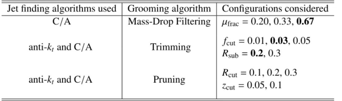
The configurations of the grooming algorithms described above are given in Table
1. Furthermore,six additional pruning configurations closer to the values used in Refs. [8,13] were also tested, but exhibit a negligible impact on the pile-up dependence of the jet mass and properties as discussed in Section
3.2.Jet finding algorithms used Grooming algorithm Configurations considered C/A Mass-Drop Filtering
µfrac=0.20, 0.33,
0.67anti-k
tand C/A Trimming f
cut=0.01,
0.03, 0.05R
sub=0.2, 0.3anti-k
tand C/A Pruning R
cut=0.1, 0.2, 0.3
z
cut=0.05, 0.1
Table 1: Summary of the grooming configurations considered in this study. Values in boldface are optimized configurations reported in Ref. [12] and Ref. [14] for filtering and trimming, respectively.
3.2 Dependence of the Jet Energy Scale and the Jet Mass Scale on pile-up
The jet mass may be calibrated using MC-based calibration factors derived as a function of the jet p
jetTand
η[11]. This section elaborates on the magnitude and variation of the impact of pile-up on the jet mass and other observables and the extent to which trimming, filtering, and pruning are able to minimize those effects. In particular, this measure of performance is used as one of the primary figures of merit in determining a subset of groomed jet algorithms on which to focus for physics analysis in ATLAS.
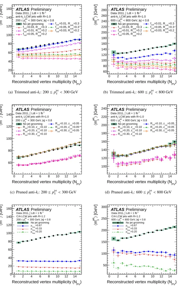
Figure
1shows the dependence of the mean uncalibrated jet mass,
hmjeti, on the number of recon-structed primary vertices, N
PV, for jets in the central region
|η|<0.8. This dependence is shown in two p
jetTranges of interest for jets after trimming, filtering, and pruning. For these comparisons, only the final period of data collection from 2011 is used, which corresponds to approximately 1 fb
−1of integrated luminosity but represents the period with the highest instantaneous luminosity recorded at
√s
=7 TeV.
The lower range, 200
≤p
jetT <300 GeV, represents the threshold for most hadronic boosted object mea- surements and searches, whereas the range 600
≤p
jetT <800 GeV is expected to contain top quarks for which the decay products will be fully merged within an R
=1.0 jet nearly 100% of the time [11]. In each figure, the full set of grooming algorithm parameter settings is included for comparison. As noted in Table
1, two values of the subjet radius,R
sub, are used for trimming, three R
cutfactors for pruning are tested, and three
µfracsettings are evaluated using the filtering algorithm.
Several observations can be made from Figure
1. Trimming and filtering both have a significantimpact on the strong rise for ungroomed jets of
hmjetiwith pile-up, whereas pruning does not. For at
least one of the configurations tested, trimming and filtering are both able to reduce this dependence to
approximately zero, as measured by the slope of
hmjetiversus N
PV. Furthermore, the trimming configu-
rations tested provide a highly tunable set of parameters that allow for a relatively continuous adjustment
from small to large reduction of the pile-up dependence of the jet mass. The parameter settings with
R
sub =0.2, f
cut =0.03 and R
sub =0.3, f
cut =0.05 exhibit good stability for both low and high p
jetT, with
the f
cut =0.05 configuration exhibiting a slightly smaller impact from pile-up at high N
PVfor low p
jetT.
The other parameter settings either do not reduce the pile-up dependence at low p
jetT(e.g. f
cut=0.01) or
PV) Reconstructed vertex multiplicity (N
0 2 4 6 8 10 12 14
[GeV]〉jet m〈
20 40 60 80 100 120 140
160 ATLAS Preliminary
Ldt = 1 fb-1
∫ Data 2011,
LCW jets with R=1.0 anti-kt
| < 0.8 η < 300 GeV, |
T
pjet
≤ 200
No jet grooming =0.3
=0.01, Rsub
fcut sub=0.3
=0.03, R
fcut =0.3
=0.05, Rsub
fcut sub=0.2
=0.01, R
fcut =0.2
=0.03, Rsub
fcut sub=0.2
=0.05, R fcut
(a) Trimmed anti-kt: 200≤pjetT <300 GeV
PV) Reconstructed vertex multiplicity (N
0 2 4 6 8 10 12 14
[GeV]〉 1 jet m〈
60 80 100 120 140 160 180 200 220 240 260
280 ATLAS Preliminary
Ldt = 1 fb-1
∫ Data 2011,
LCW jets with R=1.0 anti-kt
| < 0.8 η < 800 GeV, |
T
pjet
≤ 600
No jet grooming =0.3
=0.01, Rsub
fcut sub=0.3
=0.03, R
fcut =0.3
=0.05, Rsub
fcut sub=0.2
=0.01, R
fcut =0.2
=0.03, Rsub
fcut sub=0.2
=0.05, R fcut
(b) Trimmed anti-kt: 600≤pjetT <800 GeV
PV) Reconstructed vertex multiplicity (N
0 2 4 6 8 10 12 14
[GeV]〉jet m〈
60 80 100 120 140
ATLAS Preliminary
Ldt = 1 fb-1
∫ Data 2011,
LCW jets with R=1.0 anti-kt
| < 0.8 η < 300 GeV, |
T
pjet
≤ 200
No jet grooming =0.05
=0.10, zcut
Rcut
=0.10
=0.10, zcut
Rcut =0.05
=0.20, zcut
Rcut
=0.10
=0.20, zcut
Rcut =0.05
=0.30, zcut
Rcut
=0.10
=0.30, zcut
Rcut
(c) Pruned anti-kt: 200≤pjetT <300 GeV
PV) Reconstructed vertex multiplicity (N
0 2 4 6 8 10 12 14
[GeV]〉 1 jet m〈
100 120 140 160 180 200 220
240 ATLAS Preliminary
Ldt = 1 fb-1
∫ Data 2011,
LCW jets with R=1.0 anti-kt
| < 0.8 η < 800 GeV, |
T
pjet
≤ 600
No jet grooming =0.05
=0.10, zcut
Rcut
=0.10
=0.10, zcut
Rcut =0.05
=0.20, zcut
Rcut
=0.10
=0.20, zcut
Rcut =0.05
=0.30, zcut
Rcut
=0.10
=0.30, zcut
Rcut
(d) Pruned anti-kt: 600≤pjetT <800 GeV
PV) Reconstructed vertex multiplicity (N
0 2 4 6 8 10 12 14
[GeV]〉jet m〈
0 20 40 60 80 100 120 140
160 ATLAS Preliminary
Ldt = 1 fb-1
∫ Data 2011,
C/A LCW jets with R=1.2
| < 0.8 η < 300 GeV, |
T
pjet
≤ 200
No jet grooming
=0.67 µfrac
=0.33 µfrac
=0.20 µfrac
(e) Filtered C/A: 200≤pjetT <300 GeV
PV) Reconstructed vertex multiplicity (N
0 2 4 6 8 10 12 14
[GeV]〉 1 jet m〈
50 100 150 200 250
300 ATLAS Preliminary
Ldt = 1 fb-1
∫ Data 2011,
C/A LCW jets with R=1.2
| < 0.8 η < 800 GeV, |
T
pjet
≤ 600
No jet grooming
=0.67 µfrac
=0.33 µfrac
=0.20 µfrac
(f) Filtered C/A: 600≤pjetT <800 GeV
Figure 1: Evolution of the mean jet mass,
hmjeti, for jets in the central region|η| <0.8 as a function of the reconstructed vertex multiplicity, N
PVfor leading jets in the range 200
≤p
jetT <300 GeV (left) and the range 600
≤p
jetT <800 GeV (right).
(a)-(b)show trimmed anti-k
tjets with R
=1.0,
(c)-(d)show pruned anti-k
tjets with R
=1.0, and
(e)-(f)show split and filtered C/A jets with R
=1.2. The error bars indicate the statistical uncertainty on the mean value in each bin.
6
result in a downward slope of
hmjetias a function of pile-up at high p
jetT(e.g. f
cut=0.05, R
sub=0.2 and
µfrac=0.20).
Pruning, on the other hand, exhibits the smallest impact on the pile-up dependence of the jet mass.
Only by increasing the z
cutparameter from z
cut =0.05 to z
cut =0.10 can any reduction on the depen- dence of
hmjetion pile-up be observed. This change is equivalent to reducing the fraction of low p
Tcontributions during the jet recombination; in the language of trimming, this is analogous to raising f
cut. This change reduces the magnitude of the variation of the mean jet mass as a function N
PVfor low p
jetTslightly. Interestingly, the R
cutparameter gives very little impact on the performance, with nearly all of the differences observed being due to the change in z
cut. This observation holds for both low and high
p
jetT.
The mass-drop filtering algorithm can be made to a
ffect significantly
hmjetisolely via the mass-drop criterion,
µfrac. A drastic change in
hmjetiis observed for all configurations of the jet filtering, with the strictest
µfrac=0.20 setting rejecting nearly 90% of the jets considered and resulting in a slight negative slope in the mean jet mass versus pile-up. Nevertheless, the other two settings of
µfractested in these studies exhibit no significant variation as a function of the number of reconstructed vertices, and the optimum value of
µfrac=0.67 seems to exhibit the greatest stability. Studies from 2010 [10] demonstrate that this reduction in the sensitivity to pile-up is due primarily to the filtering step in the algorithm as opposed to the jet selection itself.
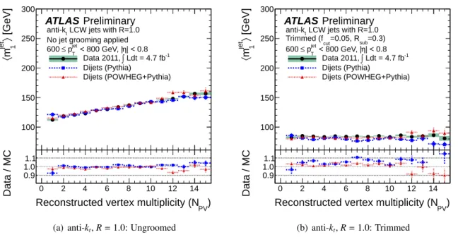
Figure
2presents the pile-up dependence of
hmjet1 iin data compared to two MC generators. Here, only the range 600
≤p
jetT <800 GeV for ungroomed and trimmed anti-k
tjets is shown for brevity, but similar conclusions apply in all p
jetTranges. The comparison is made using the full 4.7 fb
−1of integrated luminosity collected in 2011. PYTHIA and POWHEG both model the data fairly accurately, with a slight 5%–10% discrepancy appearing in the prediction from PYTHIA for the trimmed jets. Most importantly, the impact of pile-up is very well modeled, with the slopes of the
hmjet1 iversus N
PVagreeing to within 3% compared to POWHEG
+PYTHIA for both ungroomed and trimmed jets.[GeV]〉 1 jet m〈
100 150 200 250 300
PV) Reconstructed vertex multiplicity (N
0 2 4 6 8 10 12 14
Data / MC
0.9 1.0 1.1
ATLAS Preliminary
LCW jets with R=1.0 anti-kt
No jet grooming applied
| < 0.8 η < 800 GeV, |
T
pjet
≤ 600
Ldt = 4.7 fb-1
∫ Data 2011, Dijets (Pythia)
Dijets (POWHEG+Pythia)
(a) anti-kt,R=1.0: Ungroomed
[GeV]〉 1 jet m〈
100 150 200 250 300
PV) Reconstructed vertex multiplicity (N
0 2 4 6 8 10 12 14
Data / MC
0.9 1.0 1.1
ATLAS Preliminary
LCW jets with R=1.0 anti-kt
=0.3)
=0.05, Rsub
Trimmed (fcut
| < 0.8 η < 800 GeV, |
T
pjet
≤ 600
Ldt = 4.7 fb-1
∫ Data 2011, Dijets (Pythia)
Dijets (POWHEG+Pythia)
(b) anti-kt,R=1.0: Trimmed
Figure 2: Dependence of the mean jet mass,
hmjeti, on the reconstructed vertex multiplicity for anti-k
tjets with R
=1.0 in the range 600
≤p
jetT <800 GeV in the central region
|η| <0.8. Both
(a)untrimmed
anti-k
tjets and
(b)trimmed anti-k
tjets with f
cut=0.05 show good agreement between data and MC. The
error bars indicate the statistical uncertainty on the mean value in each bin.
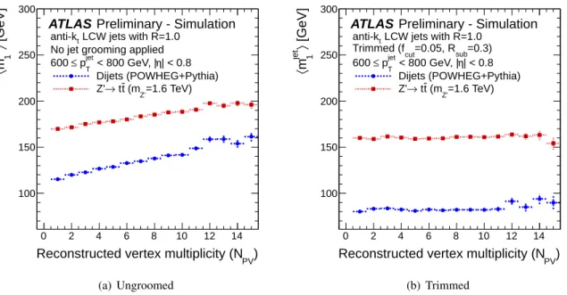
Beyond simply providing a pile-up-independent average jet mass, the optimal grooming configura- tions render the full jet mass spectrum insensitive to high instantaneous luminosity. Figure
3demon- strates this by comparing the jet mass spectrum for leading ungroomed and trimmed anti-k
tjets. The comparison is performed both in data and using the Z
0 →t¯ t MC sample. The result using the inclusive jet sample obtained from data shows that a nearly identical trimmed m
jetspectrum is obtained regardless of the level of pile-up. The peak of the leading jet mass distribution for events with N
PV ≥12 is shifted comparatively more due to trimming: from m
jet ≈125 GeV to m
jet ≈45 GeV as compared to an initial peak position of m
jet ≈90 GeV for events with 1
≤N
PV ≤4. Nonetheless, the resulting trimmed jet mass spectra exhibit no dependence on N
PV.
1
Leading jet mass, mjet
0 50 100 150 200 250 300
Arbitrary units
0 0.02 0.04 0.06 0.08 0.1
ATLAS Preliminary
Ldt = 4.7 fb-1
∫ Data 2011,
with R=1.0 LCW, No jet grooming anti-kt
| < 0.8 η < 800 GeV, |
T
pjet
≤ 600
≤4 NPV
≤ 1
≤7 NPV
≤ 5
≤11 NPV
≤ 8
≥12 NPV
(a) Data: anti-kt,R=1.0: Ungroomed
1
Leading jet mass, mjet
0 50 100 150 200 250 300
Arbitrary units
0 0.02 0.04 0.06 0.08 0.1 0.12
0.14 ATLAS Preliminary
Ldt = 4.7 fb-1
∫ Data 2011,
sub=0.3
=0.05, R with R=1.0 LCW, fcut
anti-kt
| < 0.8 η < 800 GeV, |
T
pjet
≤ 600
≤4 NPV
≤ 1
≤7 NPV
≤ 5
≤11 NPV
≤ 8
≥12 NPV
(b) Data: anti-kt,R=1.0: Trimmed
1
Leading jet mass, mjet 120 140 160 180 200 220 240 260
Arbitrary units
0 0.02 0.04 0.06 0.08 0.1 0.12 0.14 0.16
0.18 ATLAS Preliminary - Simulation
= 1.6 TeV) (mZ'
t
→ t Z'
with R=1.0 LCW, No jet grooming anti-kt
| < 0.8 η < 800 GeV, |
T
pjet
≤ 600
≤4 NPV
≤ 1
≤7 NPV
≤ 5
≤11 NPV
≤ 8
≥12 NPV
(c)Z0: anti-kt,R=1.0: Ungroomed
1
Leading jet mass, mjet 120 140 160 180 200 220 240 260
Arbitrary units
0 0.02 0.04 0.06 0.08 0.1 0.12 0.14 0.16
0.18 ATLAS Preliminary - Simulation
= 1.6 TeV) (mZ'
t
→ t Z'
sub=0.3
=0.05, R with R=1.0 LCW, fcut
anti-kt
| < 0.8 η < 800 GeV, |
T
pjet
≤ 600
≤4 NPV
≤ 1
≤7 NPV
≤ 5
≤11 NPV
≤ 8
≥12 NPV
(d)Z0: anti-kt,R=1.0: Trimmed
Figure 3: Jet mass spectra for four primary vertex multiplicity ranges for anti-k
tjets with R
=1.0 in the range 600
≤p
jetT <800 GeV. Both untrimmed anti-k
tjets (left) and trimmed anti-k
tjets (right) are compared for the various N
PVranges in data (top) and for a Z
0→t¯ t sample (bottom).
8
Comparisons performed using the Z
0 →t¯ t sample demonstrate the same performance of the trimming algorithm, but in the context of the reconstruction of highly boosted top quarks. Figures
3(c)-(d)indicate that the ability to render the full jet mass distribution independent of pile-up does not come at the cost of the mass resolution or scale. Prior to jet trimming, a shift in the peak position of the jet mass of nearly 15 GeV is observed between the lowest and the highest ranges of N
PVstudied. After jet trimming, each of the resulting mass spectra for the various N
PVranges are narrower and lie directly on top of one another, even in the case of a jet containing a highly boosted, and thus very collimated, top quark decay. This observation, combined with that above, demonstrates that the trimming algorithm is working as expected by removing soft, wide-angle contributions to the jet mass while retaining the relevant hard substructure of the jet.
Finally, although not shown explicitly, the same observations made here for the resilience of the trimmed jet mass spectrum can also be made for the filtered jet mass.
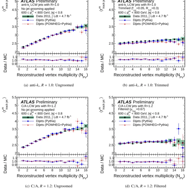
The method used to determine the mass scale uncertainty is discussed at length in Ref. [11]. The approach utilizes the ratio of the calorimeter m
jetto the track jet mass, which measures the same quantity as in Eq. (1) but using tracks as input to the jet algorithm instead of clusters. The mass ratio, r
track jetm, is defined explicitly as
r
track jetm =m
jetm
track jet.(2)
The matching between calorimeter and track jets is performed using a matching radius of
∆R
<0.3 in
η−φcoordinates. The ratio in Eq. (2) is expected to be well described by the detector simulation in the case that detector e
ffects are well modeled. That is to say, even if some underlying physics process were unaccounted for by the MC simulation, then as long as this process a
ffects both the track jet mass and the calorimeter jet mass, then the ratio of data to MC should be relatively unaffected. The double ratio of r
mtrack jetevaluated in the data to that evaluated in the MC simulation is constructed to test this.
Systematic e
ffects on the calibration of these jets are estimated via deviations between data and MC for the dependence of r
mtrack jeton p
jetTand m
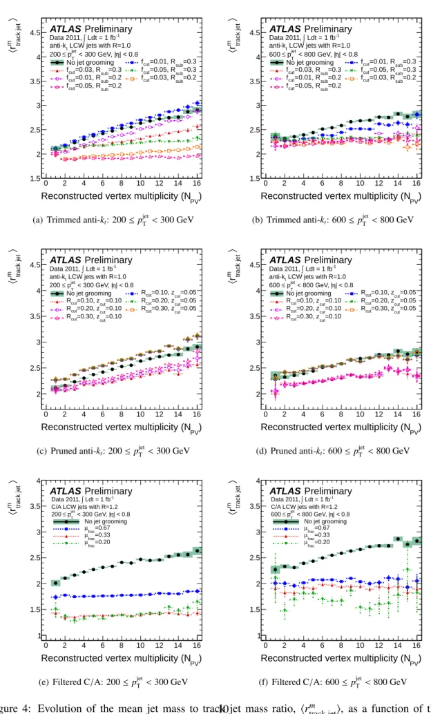
jet. In Figure
4, the dependence of the mean value ofr
mtrack jeton N
PVis evaluated for trimming, filtering, and pruning for two p
jetTranges of interest. This is analogous to Figure
1, but isolates the impact of pile-up on the mass itself on a jet-by-jet basis given thatm
track jetfor each jet is not affected by pile-up, to first order.
Figure
4demonstrates that trimming and filtering both provide robust jet definitions in the presence of high luminosity. r
mtrack jetis observed to be nearly equal among the various trimming configurations in the case of little or no in-time pile-up (i.e. N
PV ≈1) whereas filtering shows a significant, although small, di
fference between the configurations using
µfrac =0.67, 0.33, 0.20. This shows that the filtering method does affect the magnitude of m
jetand m
track jetslightly differently, resulting in an approximate 12% relative drop in
hrmtrack jetiafter filtering. As indicated in Figure
5, these distributions are nonethelesswell modeled by the MC simulation, resulting in double ratios of data to MC very close to one (shown in the bottom panels in Figure
5). The trimming configuration withR
sub=0.3, f
cut=0.01 has almost no impact on the dependence of r
mtrack jetwith pile-up.
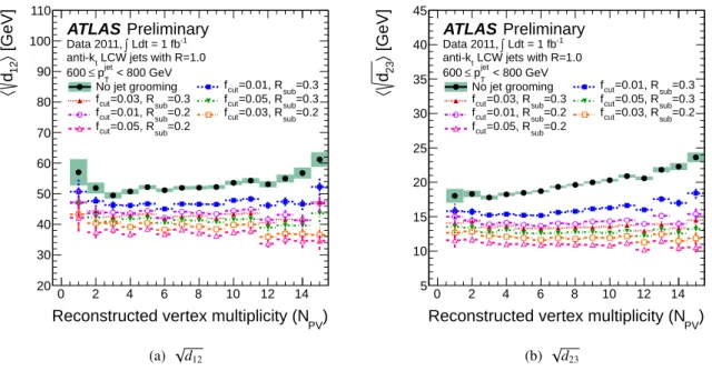
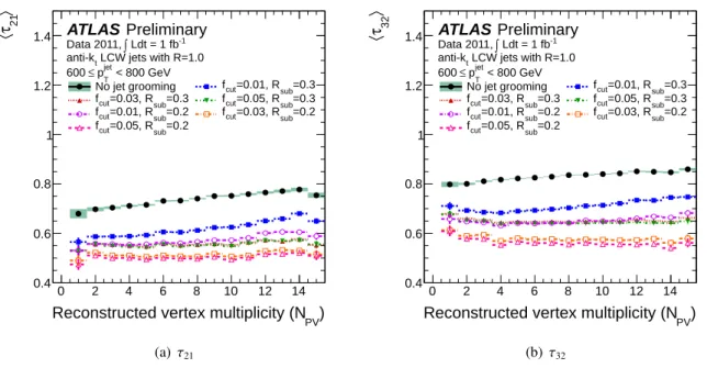
3.3 Jet Substructure Properties
Searches and measurements that utilize the information encoded in the jet mass can often also benefit from more detailed and potentially complex measures of jet substructure. Two such observables are
pd
i jand
τN. The family of
pd
i jvariables, most often seen in the form of
√d
12or
√d
23, classify the massive “scales” of a given jet. For example, the expected value for a two-body heavy particle decay is approximately
√d
12 ≈m
jet/2 [11], whereas jets formed from the parton shower of light quarks andgluons will tend to exhibit a steeply falling spectrum of both
√d
12and
√d
23. These are defined by
PV) Reconstructed vertex multiplicity (N
0 2 4 6 8 10 12 14 16
〉m track jetr〈
1.5 2 2.5 3 3.5 4
4.5 ATLAS Preliminary
Ldt = 1 fb-1
∫ Data 2011,
LCW jets with R=1.0 anti-kt
| < 0.8 η < 300 GeV, |
T
pjet
≤ 200
No jet grooming =0.3
=0.01, Rsub
fcut sub=0.3
=0.03, R
fcut =0.3
=0.05, Rsub
fcut sub=0.2
=0.01, R
fcut =0.2
=0.03, Rsub
fcut sub=0.2
=0.05, R fcut
(a) Trimmed anti-kt: 200≤pjetT <300 GeV
PV) Reconstructed vertex multiplicity (N
0 2 4 6 8 10 12 14 16
〉m track jetr〈
1.5 2 2.5 3 3.5 4
4.5 ATLAS Preliminary
Ldt = 1 fb-1
∫ Data 2011,
LCW jets with R=1.0 anti-kt
| < 0.8 η < 800 GeV, |
T
pjet
≤ 600
No jet grooming =0.3
=0.01, Rsub
fcut sub=0.3
=0.03, R
fcut =0.3
=0.05, Rsub
fcut sub=0.2
=0.01, R
fcut =0.2
=0.03, Rsub
fcut sub=0.2
=0.05, R fcut
(b) Trimmed anti-kt: 600≤pjetT <800 GeV
PV) Reconstructed vertex multiplicity (N
0 2 4 6 8 10 12 14 16
〉m track jetr〈
2 2.5 3 3.5 4
4.5 ATLAS Preliminary
Ldt = 1 fb-1
∫ Data 2011,
LCW jets with R=1.0 anti-kt
| < 0.8 η < 300 GeV, |
T
pjet
≤ 200
No jet grooming =0.05
=0.10, zcut
Rcut
=0.10
=0.10, zcut
Rcut =0.05
=0.20, zcut
Rcut
=0.10
=0.20, zcut
Rcut =0.05
=0.30, zcut
Rcut
=0.10
=0.30, zcut
Rcut
(c) Pruned anti-kt: 200≤pjetT <300 GeV
PV) Reconstructed vertex multiplicity (N
0 2 4 6 8 10 12 14 16
〉m track jetr〈
2 2.5 3 3.5 4
4.5 ATLAS Preliminary
Ldt = 1 fb-1
∫ Data 2011,
LCW jets with R=1.0 anti-kt
| < 0.8 η < 800 GeV, |
T
pjet
≤ 600
No jet grooming =0.05
=0.10, zcut
Rcut
=0.10
=0.10, zcut
Rcut =0.05
=0.20, zcut
Rcut
=0.10
=0.20, zcut
Rcut =0.05
=0.30, zcut
Rcut
=0.10
=0.30, zcut
Rcut
(d) Pruned anti-kt: 600≤pjetT <800 GeV
PV) Reconstructed vertex multiplicity (N
0 2 4 6 8 10 12 14 16
〉m track jetr〈
1 1.5 2 2.5 3 3.5 4
ATLAS Preliminary
Ldt = 1 fb-1
∫ Data 2011,
C/A LCW jets with R=1.2
| < 0.8 η < 300 GeV, |
T
pjet
≤ 200
No jet grooming
=0.67 µfrac
=0.33 µfrac
=0.20 µfrac
(e) Filtered C/A: 200≤pjetT <300 GeV
PV) Reconstructed vertex multiplicity (N
0 2 4 6 8 10 12 14 16
〉m track jetr〈
1 1.5 2 2.5 3 3.5 4
ATLAS Preliminary
Ldt = 1 fb-1
∫ Data 2011,
C/A LCW jets with R=1.2
| < 0.8 η < 800 GeV, |
T
pjet
≤ 600
No jet grooming
=0.67 µfrac
=0.33 µfrac
=0.20 µfrac
(f) Filtered C/A: 600≤pjetT <800 GeV
Figure 4: Evolution of the mean jet mass to track jet mass ratio,
hrmtrack jeti, as a function of the re-constructed vertex multiplicity, N
PVfor the range 200
≤p
jetT <300 GeV range (left), and the range 600
≤p
jetT <800 GeV (right).
(a)-(b)show trimmed anti-k
tjets with R
=1.0,
(c)-(d)show pruned anti-k
tjets with R
=1.0, and
(e)-(f)show split and filtered C/A jets with R
=1.2. The error bars indicate the statistical uncertainty on the mean value in each bin.
10
〉m track jetr〈
2 2.5 3 3.5 4 4.5 5
PV) Reconstructed vertex multiplicity (N
0 2 4 6 8 10 12 14 16
Data / MC
0.9 1.0 1.1
ATLAS Preliminary
LCW jets with R=1.0 anti-kt
No jet grooming applied
| < 0.8 η < 800 GeV, |
T
pjet
≤ 600
Ldt = 4.7 fb-1
∫ Data 2011, Dijets (Pythia)
Dijets (POWHEG+Pythia)
(a) anti-kt,R=1.0: Ungroomed
〉m track jetr〈
2 2.5 3 3.5 4 4.5 5
PV) Reconstructed vertex multiplicity (N
0 2 4 6 8 10 12 14 16
Data / MC
0.9 1.0 1.1
ATLAS Preliminary
LCW jets with R=1.0 anti-kt
=0.3)
=0.05, Rsub
Trimmed (fcut
| < 0.8 η < 800 GeV, |
T
pjet
≤ 600
Ldt = 4.7 fb-1
∫ Data 2011, Dijets (Pythia)
Dijets (POWHEG+Pythia)
(b) anti-kt,R=1.0: Trimmed
〉m track jetr〈
2 2.5 3 3.5 4 4.5 5 5.5
PV) Reconstructed vertex multiplicity (N
0 2 4 6 8 10 12 14 16
Data / MC
0.9 1.0 1.1
ATLAS Preliminary
C/A LCW jets with R=1.2 No jet grooming applied
| < 0.8 η < 800 GeV, |
T
pjet
≤ 600
Ldt = 4.7 fb-1
∫ Data 2011, Dijets (Pythia)
Dijets (POWHEG+Pythia)
(c) C/A,R=1.2: Ungroomed
〉m track jetr〈
2 2.5 3 3.5 4 4.5 5 5.5
PV) Reconstructed vertex multiplicity (N
0 2 4 6 8 10 12 14 16
Data / MC
0.9 1.0 1.1
ATLAS Preliminary
C/A LCW jets with R=1.2
=0.67) µfrac
Filtered (
| < 0.8 η < 800 GeV, |
T
pjet
≤ 600
Ldt = 4.7 fb-1
∫ Data 2011, Dijets (Pythia)
Dijets (POWHEG+Pythia)
(d) C/A,R=1.2: Filtered