Pile-up corrections for jets from proton-proton collisions at √

(1)

ATLAS-CONF-2012-064 04July2012

ATLAS NOTE

ATLAS-CONF-2012-064

July 2, 2012

Pile-up corrections for jets from proton-proton collisions at √

s = 7 TeV in ATLAS in 2011

The ATLAS Collaboration

Abstract

The high luminosity and high total proton-proton interaction cross section at

√

s=

7 TeV at the LHC lead to multiple proton collisions per bunch crossing. With instantaneous lumi- nosities reaching up to 3.6

×

10

³³

cm

⁻²

s

⁻¹

in 2011, the number of these pile-up interactions increased significantly with respect to 2010. Particles from these interactions are scattered into the ATLAS calorimeters independently of the particle flow from the (triggered) hard- scatter interaction, and add approximately 370(850) MeV per reconstructed primary ver- tex to the transverse momentum (p

T

) of a jet reconstructed with the anti-k

t

algorithm with

R=

0.4(0.6) in the central region of the detector. In addition to the effect of pile-up interac- tions in the same bunch crossing as the hard scatter, in 2011 the 50 ns proton bunch spacing within LHC bunch trains introduced a sensitivity of the calorimeter signals to the energy flow in past collisions, due to the ATLAS calorimeter signal shapes. The resulting increase of the reconstructed jet

p_T

per additional interaction in the central region is approximately 60(210) MeV, while in the forward region a decrease of approximately 350(470) MeV is observed. Monte Carlo simulation-based algorithms have been developed to address both effects on the jet signal individually and independently. Results from in-situ validation tech- niques in 2011 data indicate that the modeling of these effects is not perfect, and the resulting systematic bias in the jet

pT

measurement is at most 3% for

pT >

40 GeV at the highest pile-up activities experienced in 2011.

Reproduction of this article or parts of it is allowed as specified in the CC-BY-3.0 license.

(2)

1 Introduction

Jets are the dominant final state objects of high-energy proton-proton (pp) interactions at the Large Hadron Collider (LHC) at CERN. They are key ingredients for many physics measurements and for searches for new phenomena. Jets are observed as groups of topologically-related energy deposits in the ATLAS [1] calorimeters, most of which are associated with tracks of charged particles as measured in the inner detector. They are reconstructed with the anti-k

_t

algorithm [2] and calibrated using a combination of methods based on Monte Carlo simulation as well as in-situ techniques. All relevant details of the jet reconstruction in ATLAS can be found in Ref. [3].

In 2011, ATLAS collected signals from pp collisions at a center-of-mass energy of

√

s

=

7 TeV, with total statistics corresponding to approximately 5 fb

⁻¹

of integrated luminosity. This large data set allows significant gains in the precision of the jet energy measurement by fully exploiting in-situ techniques for calibration, such as transverse momentum balance in

γ+jet,

Z+jet and di-jet events. On the other hand, the beam conditions in 2011 were more challenging than in 2010. The instantaneous luminosity reached values of 3.6

×

10

³³

cm

⁻²

s

⁻¹

, generating an average number of pp collisions per bunch crossing of

µ ≈

8. These additional interactions resulted in additional signals in the ATLAS detectors, overlapping with those from the hard-scatter process (in-time pile-up). Furthermore, the short LHC bunch-crossing intervals of 50 ns introduced a small yet observable sensitivity of the calorimeter signals to the collision history in previous bunch crossings, especially in the ATLAS liquid argon calorimeters with their long (bipolar) shaped signal baseline of approximately 600 ns (out-of-time pile-up) [4].

In this note, a jet energy scale (JES) correction derived from Monte Carlo (MC) simulation and intended to suppress both in-time and out-of-time pile-up signal contributions to jets is described. This MC based approach has the advantage that it is possible to determine corrections for all jets reconstructed within the full calorimeter acceptance of ATLAS, i.e. the pseudorapidity (η

det

) range

|ηdet|<

4.9. Alter- native methods using measures for pile-up contributions to jets from e.g. reconstructed tracks pointing to the jet are under study, but limited in their application to the region covered by the ATLAS inner detector (

|ηdet|<

2.5).

The note begins with a brief description of the collision data that were used and the conditions in which they were recorded in Section 2, followed by the configuration of the Monte Carlo samples that were used in Section 3 and a brief overview on the jet reconstruction and calibration in ATLAS in Section 4. The event selection is described in Section 5. The description of the pile-up correction method can be found in Section 6, followed by a discussion of the systematic bias due to imperfect modeling of the effects of pile-up on jets in Section 7. Finally, a summary of the note is provided in Section 8.

The correction described here is only one link in the chain of calibrations and corrections applied to fully calibrate jets in ATLAS. Additional response corrections derived in-situ from transverse momentum ( p

T

) balances in

γ+jet [5],

Z+jet [6], di-jet, and multi-jet final states are combined to form the full JES correction. The resulting combined systematic JES uncertainty can be considerably smaller than the systematic bias presented here, due to additional constraints from kinematic features of the various final states considered.

It should also be emphasized that the corrections described here are derived based on the transverse

momentum contribution of pile-up to jets. The jet energy after correction is then the original energy

scaled according to the change of transverse momentum imposed by the pile-up correction. Any partic-

ular effect of pile-up on the jet mass, which may show significantly different modifications and therefore

require more sophisticated methods possibly including jet grooming techniques aiming at removing jet

constituents associated with pile-up, is thus not specifically corrected.

(3)

2 Experimental data

The ATLAS experiment features a multi-purpose detector designed to precisely measure individual par- ticles and particle jets produced in the pp collisions at the LHC. From inside out, the detector consists of an inner tracking detector, surrounded by electromagnetic sampling calorimeters. Those in turn are sur- rounded by hadronic sampling calorimeters and, behind those, an air-toroid muon detector. The ATLAS calorimeters provide coverage hermetic in azimuth in the pseudorapidity range

|η_det| <

4.9. A detailed description of the ATLAS detector can be found in Ref. [1].

One feature important for the pile-up signal contribution in 2011 is the sensitivity of the ATLAS liquid argon calorimeters to the bunch crossing history. In any liquid argon calorimeter cell, the re- constructed energy is sensitive to the pp interactions occurring in approximately 24 preceding and one immediately following bunch crossings, in addition to pile-up interactions in the current bunch cross- ing. This is due to the relatively long charge collection time in these calorimeters (typically 400 ns), as compared to the bunch crossing intervals at the LHC (design 25 ns and actually 50 ns in 2011 data). To reduce this sensitivity, a fast, bi-polar shaped signal is used with net zero integral over time.

The signal shapes in the liquid argon calorimeters have been optimized for this purpose, thus on average resulting in cancellation of in-time and out-of-time pile-up in any given calorimeter cell. By design of the shaping amplifier, the most efficient suppression is achieved for 25 ns bunch spacing in the LHC beams. The 2011 beam conditions, with 50 ns bunch spacing and a relatively low occupancy from the instantaneous luminosities achieved, therefore do not allow for full pile-up suppression by signal shaping, in particular in the central calorimeter region. Pile-up suppression is further limited by large fluctuations in the number of additional interactions from bunch crossing to bunch crossing, and the energy flow patterns of the individual collisions in the time window of sensitivity

¹

of approximately 600 ns. Therefore, the shaped signal extracted by digital filtering shows a residual sensitivity to in-time and out-of-time pile-up. This sensitivity is further enhanced by the noise suppression implemented in the calorimeter signal definition presented in Section 4 and further discussed in the context of the pile-up suppression strategy in Section 6. All details of the ATLAS liquid argon calorimeter readout and signal processing can be found in Ref [4].

The data used in this study were recorded by ATLAS between May and October 2011, with the LHC running with 50 ns bunch spacing, and bunches organized in bunch trains. The average number of interactions per bunch crossing throughout the data-taking period considered was approximately 3

≤ µ ≤

8 until summer 2011, with a global average for this period of

µ≈

6. Starting in August 2011 and lasting through the end of the proton run,

µ

ranged from approximately 5 to 17, with an average of about 12. The total amount of proton collision data collected by ATLAS in 2011 corresponds to an integrated luminosity of 5 fb

⁻¹

.

3 Monte Carlo simulation

The jet and photon samples used for this study are generated with the P

ythia

6 [7] event generator. The proton parton distribution function (PDF) set used is the modified leading order PDF set MRST LO** [8].

The parton shower and multiple parton interactions in the underlying event have been tuned to first LHC data (Pythia tune AUET2B with MRST LO** PDFs) [9].

Minimum bias events are generated using P

ythia

8 [10] with the 4C tune [11] and MRST LO** PDF.

These minimum bias events are used to form pile-up events, which are overlaid onto the hard-scatter events following a Poisson distribution around the average number of additional pp collisions per bunch crossing measured in the experiment. The LHC bunch train structure with 36 proton bunches per train and 50 ns spacing between the bunches, is also modeled by organizing the simulated collisions into four

1The shaped pulse has a duration exceeding the charge collection time.

(4)

such trains. This allows the inclusion of out-of-time pile-up effects driven by the distance of the hard scatter events from the beginning of the bunch train. The first ten bunch crossings, approximately, are characterized by increasing out-of-time pile-up contributions from the collision history getting filled with an increasing number of bunch crossings with pp interactions. For the remaining

≈

26 bunch crossings in a train this out-of-time pile-up contribution is stable within the bunch-to-bunch fluctuations in proton intensity at the LHC. These proton bunch intensity variations are not included in the simulation.

The G

eant

4 software toolkit [12] within the ATLAS simulation framework [13] propagates the gen- erated particles through the ATLAS detector and simulates their interactions with the detector material.

The energies deposited in active volumes of the detector are then digitized and reconstructed in a very similar fashion to the experimental data.

In general it is observed that all relevant response-related features of the experimental jet signals in ATLAS can be reasonably well described by the MC simulation generated with the tools and configura- tions discussed above, see Ref. [3] for details.

4 Jet reconstruction and calibration

Jets are reconstructed using the anti-k

t

algorithm [2] with distance parameters R

=

0.4 and R

=

0.6 from the F

ast

J

et

package [14, 15]. The four-momentum recombination scheme is used. The inputs to the jet algorithm are simulated observable particles with laboratory-frame lifetimes long enough to reach the detectors (truth jets), reconstructed tracks in the inner detector constrained to the hardest

²

primary vertex (track jets) or energy deposits in topological cell clusters (topo-clusters) [3, 16, 17] in the calorimeter. As topo-clusters can have a net negative signal, only the ones with positive energy are considered as input for jet finding.

Track jets in ATLAS can be reconstructed in various ways. In addition to just applying a standard jet algorithm to the reconstructed tracks, a dedicated algorithm that includes a vertex constraint on the track bundle forming the jet is available [18]. This particular algorithm leads to track jets exclusively assigned to one vertex.

Alternatively, and for the studies presented here, track jets are reconstructed with the same config- urations as calorimeter jets, i.e. using the anti-k

t

algorithm with R

=

0.4 and R

=

0.6, but exclusively applying the jet finding to tracks from the hardest primary vertex in the collision event. The transverse momentum of any of these track jets then provides a rather stable kinematic reference for a matching calorimeter jet, as it is independent of pile-up. Track jets can of course only be formed within the track- ing detector coverage, effectively

ηtrack jet

<

2.5

−

R. The topo-cluster formation follows cell signal significance patterns in the ATLAS calorimeters. The signal significance is measured by the absolute ratio of the cell signal to the energy equivalent noise in the cell. While in ATLAS operations prior to 2011 the cell noise was dominated by electronic noise, the short bunch crossing interval in 2011 LHC running added a noise component from bunch-to-bunch variations in the instantaneous luminosity and in the energy deposited in a given cell from previous collisions inside the window of sensitivity of the calorimeters. The cell noise thresholds steering the topo-clust- er formation thus needed to be increased from those used in 2010 to accommodate the corresponding fluctuations, which was done by raising the nominal noise:

σnoise =











σ^electronic_noise

(2010 operations)

q

σ^electronic_noise 2

+

σ^pile_noise⁻^up2

(2011 operations)

.

2This is the vertex with maximumP (p^track_T )².

(5)

η |

| 0 0.5 1 1.5 2 2.5 3 3.5 4 4.5 5

=0, DB) (MeV) µ T o t. n o is e (

1 10 10

2

10

3

10

4

FCal1 FCal2 FCal3 HEC1 HEC2 HEC3 HEC4 PS

EM1 EM2 EM3 Tile1 Tile2 Tile3

ATLAS Preliminary Simulation

(a)σnoise(|η|) in 2010 (µ=0)

η |

| 0 0.5 1 1.5 2 2.5 3 3.5 4 4.5 5

=50 ns, DB) (MeV) ∆ =8, µ T o t. n o is e (

1 10 10

2

10

3

10

4

FCal1 FCal2 FCal3 HEC1 HEC2 HEC3 HEC4 PS

EM1 EM2 EM3 Tile1 Tile2 Tile3

ATLAS Preliminary Simulation

(b)σnoise(|η|) in 2011 (µ=8)

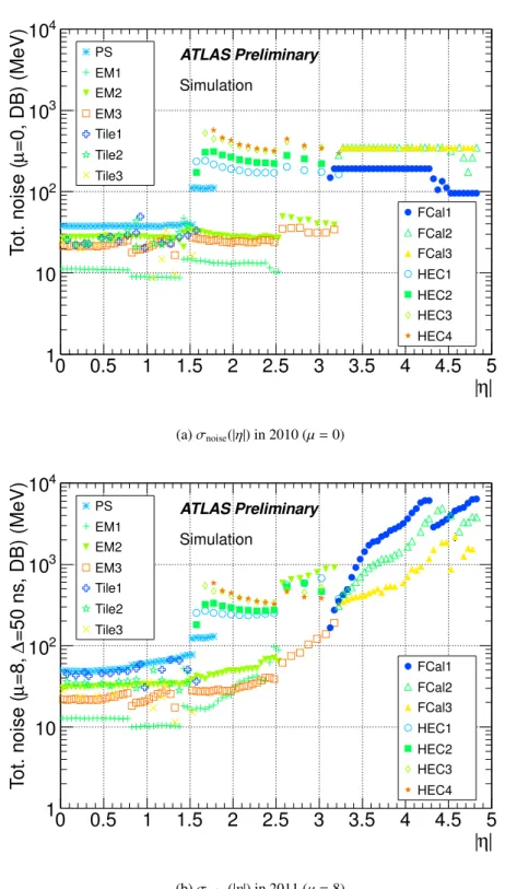
Figure 1: The energy equivalent cell noise in the ATLAS calorimeters on the EM scale, as a function of

the direction

|η|

in the detector, and for the 2010 configuration with

µ=

0 (a) and the 2011 configuration

with

µ=

8 (b). The various colors indicate the noise in the pre-sampler (PS) and the up to three layers

of

EM

calorimeter, the up to three layers of the

Tile

calorimeter, the four layers for the hadronic end-cap

(HEC) calorimeter, and the three modules of the forward (FCal) calorimeter. More details of the detector

are given in Ref. [1].

(6)

Here,

σ^electronic_noise

is the electronic noise, and

σ^pile−up_noise

the noise from pile-up, determined with MC simula- tion and corresponding to an average of eight additional pp interactions per bunch crossing (µ

=

8) in 2011. The change of the total nominal noise

σnoise

and its dependence on the calorimeter region in AT- LAS can be seen by comparing Fig. 1(a) and Fig. 1(b). In most calorimeter regions, the pile-up induced noise is smaller than or of the same magnitude as the electronic noise, with the exception of the forward calorimeters, where

σ^pile_noise⁻^up≫σ^electronic_noise

.

The implicit noise suppression implemented by the topological cluster algorithm discussed above leads to significant improvements in the calorimeter performance for e.g. the energy and spatial resolu- tions in the presence of pile-up. On the other hand, contributions from larger negative and positive signal fluctuations introduced by pile-up can survive in a given event. They thus contribute to the sensitivity to pile-up observed in the jet response, in addition to the cell-level effects mentioned in Section 2.

ATLAS has developed several calorimeter jet calibration schemes [18] with different levels of com- plexity and different sensitivity to systematic effects, which are complementary in their contribution to the jet energy measurement. The most basic scheme starts with the measured calorimeter signal at the electromagnetic (EM) energy scale [16, 19–26], which correctly measures the energy deposited by elec- tromagnetic showers.

The local cluster weighting (LCW) calibration method is based on the topo-clusters. Each cluster is classified using its location and signal density as having either electromagnetic or hadronic origin. De- pending on this classification, energy corrections derived from single charged and neutral pion simulation are applied to address non-compensation (hadronic clusters only), signal losses due to the implicit cell selections in the clustering procedure, and energy lost in non-instrumented regions close to the cluster location. The latter two corrections are specific to the cluster classification.

Both EM and LCW scale jets are then subjected to a dedicated MC-based final calibration, in which the calorimeter jet response on those scales is related to the true jet energy defined by the matching truth jet, as described in detail in Ref. [3]. After calibration, jets starting from the EM scale are referred to as EM+JES jets, while jets originally built with LCW clusters are LCW+JES jets. The final jet direction after full calibration is

η, while the direction relevant for the pile-up contributions is defined by the

position of the jet in the detector (η

det

), which is reconstructed from the EM or LCW scale kinematics before any vertex correction.

5 Event and object selection

For validation of the pile-up corrections for jets derived from MC simulation, samples of collision events with kinematic references for these jets insensitive to pile-up are extracted from data. Of particular interest here are

γ+jet events in prompt photon production, as the reconstructed photon kinematics are

not affected by pile-up, and its transverse momentum p

^γ_T

provides the stable reference for the pile-up dependent response of the balancing jet in the ratio p

^jet_T /

p

^ref_T =

p

^jet_T /p^γ_T

.

Another per jet kinematic reference is provided by the already discussed track jets from the pri- mary collision vertex matching calorimeter jets, now by the transverse momentum ratio p

^jet_T /p^ref_T =

p

^jet_T/

p

^{track jet}_T

. The corresponding jet events can be extracted from samples with central jets in the fi- nal state. Both data samples are mostly useful for validation of the pile-up correction methods, as the limited statistics and phase space coverage in 2011 do not allow direct determination of the corrections from data.

The

γ+jet sample is selected by requiring a reconstructed, high-quality isolated photon with

p

^γ_T >

25 GeV and a jet opposite it in the transverse plane (∆φ > 2.9). Events with a sub-leading jet with

p

_T >

0.2p

^γ_T

not from pile-up are rejected, to suppress contributions from large angle radiation. To

distinguish jets from the hard-scatter process from jets from pile-up in the central region of ATLAS, the

jet vertex fraction JVF is used. This variable is the ratio of the p

T

sum of tracks from the primary vertex

(7)

matched to the calorimeter jet, over the p

T

sum of all tracks matching the jet, with

|

JVF

|>

0.75 required for jets from the hard scatter process. The photon is also required to be in the central region of ATLAS, with

|η^γ| <

1.37, as is the leading jet (

|η_det| <

1.2). Further details on the

γ+jet sample selection and

quality are given in Ref. [5].

For the track jet based evaluations of the pile-up corrections, events with a calorimeter jet matching a track jet with p

^track_T >

20 GeV are extracted from an event sample triggered by high-p

T

muons, thus avoiding potential jet trigger biases. A track jet is only associated with a calorimeter jet not overlap- ping with any reconstructed muon with p

^µ_T >

5 GeV, to avoid potential biases from heavy-flavour jets containing semi-leptonic decays. The general matching criterion for track jets to calorimeter jets is

∆R= q

(η

_{track jet}−η_det

)

²+ ∆φ²_{track jet}₋_jet <

0.3. Only uniquely matched track jet-calorimeter jet pairs are considered. Outside of the imposed requirement for calorimeter jet reconstruction in ATLAS ( p

^jet_T >

10 GeV), no further cuts are applied on p

^jet_T

, to avoid biases in the p

^jet_T/

p

^track_T

ratio, in particular at low p

^track_T

.

6 Pile-up correction method

6.1 Principles

The pile-up correction method applied to reconstructed jets in ATLAS is derived from MC simulation and validated with in-situ and simulation-based techniques. The principal approach is to calculate the amount of transverse momentum generated by pile-up in a jet in MC simulation and subtract this offset

O

from the reconstructed jet p

^jet_T

at any given signal scale (EM or LCW). As all pile-up contributions to the jet signal can be considered stochastic and diffuse with respect to the true jet signal, at least to first order, both in-time and out-of-time pile-up are expected to depend only on the past and present pile-up activity, with linear relations between the amount of activity and the pile-up signal.

To characterize the in-time pile-up activity, the number of reconstructed primary vertices (N

_PV

) is used, as the ATLAS tracking detector timing resolution allows the reconstruction of only in-time tracks and vertices, so that N

PV

provides a good estimate of the actual number of proton collisions in a recorded event.

For the out-of-time pile-up activity, the average number of interactions per bunch crossing at the time of the recorded events

µ

provides a good estimator. It is derived by averaging the actual number of interactions per bunch crossing over a rather large window

∆t

in time, which safely encompasses the time interval during which the ATLAS calorimeter signal is sensitive to the activity in the collision history (∆t

≫

600 ns for the liquid argon calorimeters). The average number of interactions,

µ, can

be reconstructed from the average luminosity L over this period

∆t, the total inelastic

pp cross section (σ

_inel =

71.5 mb [27]), the number of colliding bunches in LHC (N

_bunch

) and the LHC revolution fre- quency ( f

LHC

) (see Ref. [28] for details):

µ=

L

×σinel

N

_bunch×

f

_LHC.

The jet calibration is derived for a given (reference) pile-up condition

³

(N

_PV^ref, µ^ref

) such that

O

(N

PV=

N

_PV^ref, µ= µ^ref

)

=

0. As the amount of energy scattered into a jet by pile-up and the signal modification imposed by the pile-up history determine

O

, a general dependence on the distances from the reference

3The particular choice for a working point, here (N_PV^ref = 4.9, µ^ref =5.4), is arbitrary and bears no consequence for the correction method and its uncertainty discussed in this note.

(8)

PV) Number of primary vertices (N

2 4 6 8 10

[GeV]EM TJet p

10 15 20 25 30 35 40 45 50

ATLAS Preliminary Simulation = 7 TeV s

R=0.4 Pythia Dijet, anti-kt

< 8.5 µ

≤

| < 2.1, 7.5 η

| < 25 GeV

truth

pT

≤ 20

< 30 GeV

truth

pT

≤ 25

< 35 GeV

truth

pT

≤ 30

< 40 GeV

truth

pT

≤ 35

< 45 GeV

truth

pT

≤ 40

0.003 GeV/NPV

± Average Slope = 0.288

(a)p^jet_T,EM(NPV), anti-ktjets,R=0.4 (MC)

2 4 6 8 10

[GeV]EM TJet p

10 15 20 25 30 35 40 45 50

R=0.6 Pythia Dijet, anti-kt

< 8.5 µ

≤

| < 1.9, 7.5 η

| < 25 GeV

truth

pT

≤ 20

< 30 GeV

truth

pT

≤ 25

< 35 GeV

truth

pT

≤ 30

< 40 GeV

truth

pT

≤ 35

< 45 GeV

truth

pT

≤ 40

0.003 GeV/NPV

(b)p^jet_T,EM(NPV), anti-ktjets,R=0.6 (MC)

2 4 6 8 10

[GeV]EM TJet p

20 30 40 50 60 70

ATLAS Preliminary -1

L dt = 4.7 fb

∫

= 7 TeV, s

R=0.4 Data 2011, anti-kt

< 8.5 µ

≤

| < 2.1, 7.5 η

| < 25 GeV

track jet

pT

≤ 20

< 30 GeV

track jet

pT

≤ 25

< 35 GeV

track jet

pT

≤ 30

< 40 GeV

track jet

pT

≤ 35

< 45 GeV

track jet

pT

≤ 40

0.005 GeV/NPV

(c)p^jet_T,EM(NPV), anti-ktjets,R=0.4 (data)

2 4 6 8 10

[GeV]EM TJet p

20 30 40 50 60 70

ATLAS Preliminary -1

L dt = 4.7 fb

∫

= 7 TeV, s

R=0.6 Data 2011, anti-kt

< 8.5 µ

≤

| < 1.9, 7.5 η

| < 25 GeV

track jet

pT

≤ 20

< 30 GeV

track jet

pT

≤ 25

< 35 GeV

track jet

pT

≤ 30

< 40 GeV

track jet

pT

≤ 35

< 45 GeV

track jet

pT

≤ 40

0.005 GeV/NPV

(d)p^jet_T,EM(NPV), anti-ktjets,R=0.6 (data)

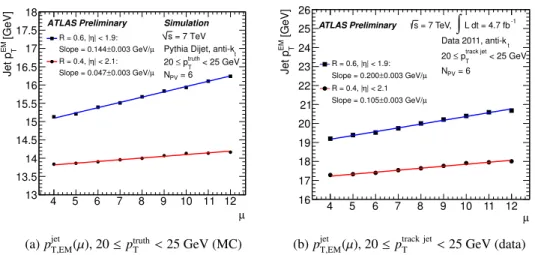
Figure 2: The average reconstructed transverse momentum p

^jet_T,EM

on EM scale for jets in MC simulation, as function of the number of reconstructed primary vertices N

PV

and 7.5

< µ <

8.5, in various bins of truth jet p

^truth_T

, for jets with R

=

0.4 (a) and R

=

0.6 (b). The dependence of p

^jet_T,EM

on N

_PV

in data, in bins of track jet transverse momentum p

^track_T

, is shown in (c) for R

=

0.4 jets, and in (d) for R

=

0.6 jets.

point is expected. From the nature of pile-up discussed earlier, the linear scaling of

O

in both N

_PV

and

µ

provides the ansatz for a correction,

O

(N

_PV, µ, η_det

)

=

p

^jet_T

(N

_PV, µ, η_det

)

−

p

^truth_T

= ∂

p

T

∂N_PV

(η

det

)

N

PV−

N

_PV^ref + ∂

p

T

∂µ

(η

det

)

µ−µ^ref

=α(η_det

)

·

N

PV−

N

_PV^ref

+β(η_det

)

·

µ−µ^ref

(1)

Here p

^jet_T,

(N

_PV, µ, η_det

) denotes the reconstructed transverse momentum of the jet in a given pile-up condi- tion (N

_PV

,µ) and at a given direction

η_det

in the detector. The true transverse momentum of the jet ( p

^truth_T

) is available from the generated particle jet matching a reconstructed jet in MC simulation. The coeffi- cients

α(ηdet

) and

β(ηdet

) only depend on

ηdet

, as both in-time and out-of-time pile-up signal contributions manifest themselves differently in different calorimeter regions, according to

•

the energy flow from collisions into that region;

(9)

•

the calorimeter granularity and occupancy after topo-cluster reconstruction, leading to different acceptances at cluster level and different probabilities for multiple particle showers to overlap in a single cluster; and

•

the effective sensitivity to out-of-time pile-up introduced by different calorimeter signal shapes.

The offset

O

can be determined in MC simulation for jets on the EM or the LCW scale by using the corresponding reconstructed transverse momentum on one of those scales, i.e. p

^jet_T =

p

^jet_T,EM

or p

^jet_T =

p

^jet_T,LCW

in Eq. 1, and p

^truth_T

. The particular choice of scale affects the magnitude of the coefficients and, therefore, the transverse momentum offset itself:

O^EM7→n

α^EM

(η

det

), β

^EM

(η

det

)

o

, O^LCW7→n

α^LCW

(η

det

), β

^LCW

(η

det

)

o .

The corrected transverse momentum of the jet at either of the two scales (p

^corr_T,EM

or p

^corr_T,LCW

) is then given by

p

^corr_T,EM =

p

^jet_T,EM− O^EM

(N

PV, µ, ηdet

) and p

^corr_T,LCW=

p

^jet_T,LCW− O^LCW

(N

PV, µ, ηdet

).

Note that after applying the correction the original p

^jet_T,EM

and p

^jet_T,LCW

dependence on N

PV

and

µ

is ex- pected to vanish in the corresponding corrected p

^corr_T,EM

and p

^corr_T,LCW

.

6.2 Deriving parameters for the correction

Figures 2(a) and (b) show the dependence of p

^jet_T,EM

, and thus

O^EM

, on N

_PV

. In this example, narrow (R

=

0.4,

|η_det| <

2.1) and wide (R

=

0.6,

|η_det| <

1.9) central jets reconstructed in MC simulation are shown for events within a given range 7.5

≤ µ <

8.5. The slopes

α^EM

are found to be independent of the true jet transverse momentum p

^truth_T

, as expected from the diffuse character of in-time pile-up signal contributions.

A qualitatively similar behavior can be observed in collision data for calorimeter jets individually matched with track jets, as described in Section 5. Here the N

_PV

dependence of p

^jet_T,EM

is measured in bins of the track jet transverse momentum p

^{track jet}_T

. The results are shown in Figs. 2(c) and (d) for the same calorimeter regions and out-of-time pile-up condition as for the MC jets in Figs. 2(a) and (b). All plots in Fig. 2 also confirm the expectation that the contributions from in-time pile-up to the jet signal are larger for wider jets (α

^EM

(R

=

0.6)

> α^EM

(R

=

0.4)), but scale only approximately with the size of the jet catchment area determined by the choice of distance parameter in the anti-k

_t

algorithm (R

=

0.4 and R

=

0.6).

The dependence of p

^jet_T,EM

on

µ, for a fixed

N

PV =

6, is shown in Fig. 3(a) for MC and Fig. 3(b) for collision data. The kinematic bins shown are the lowest bins considered, with 20

<

p

^truth_T <

25 GeV and 20

<

p

^{track jet}_T <

25 GeV for MC simulation and data, respectively. The result confirms the expectations that the dependence of p

^jet_T,EM

on the out-of-time pile-up is linear and significantly less than its dependence on the in-time pile-up contribution scaling with N

PV

. Its magnitude is still different for jets with R

=

0.6, as the size of the jet catchment area again determines the absolute contribution to p

^jet_T,EM

.

The corrections for jets calibrated with the EM+JES scheme,

α^EM

and

β^EM

, are both determined from MC simulation as functions of the jet direction

ηdet

. For this, the N

PV

dependence of p

^jet_T,EM

(η

det

) reconstructed in various bins of

µ

in the simulation is fitted and then averaged, yielding

α^EM

(η

det

). Ac- cordingly and independently, the dependence of p

^jet_T,EM

on

µ

is fitted in bins of N

PV

, yielding the average

β^EM

(η

det

), again using MC simulation. An identical procedure is used to find the correction functions

α^LCW

(η

_det

) and

β^LCW

(η

_det

) for jets calibrated with the LCW+JES scheme.

In data, both

α^EM

(α

^LCW

) and

β^EM

(β

^LCW

) can be measured using track jets, as indicated by the slopes

in Figs. 2(c), (d) and Fig. 3(b). Another in-situ approach to derive these parameters uses the variation of

(10)

µ

4 5 6 7 8 9 10 11 12

[GeV]EM TJet p

13 13.5 14 14.5 15 15.5 16 16.5 17 17.5 18

Pythia Dijet, anti-kt < 25 GeV truth pT

≤ 20

PV = 6 N

| < 1.9:

η R = 0.6, |

µ 0.003 GeV/

± Slope = 0.144

| < 2.1:

η R = 0.4, |

µ 0.003 GeV/

± Slope = 0.047

(a)p^jet_T,EM(µ), 20≤p^truth_T <25 GeV (MC)

4 5 6 7 8 9 10 11 12µ

[GeV]EM TJet p

16 17 18 19 20 21 22 23 24 25 26

ATLAS Preliminary s = 7 TeV,

∫

L dt = 4.7 fb^-1 Data 2011, anti-kt

< 25 GeV track jet pT

≤ 20

PV = 6 N

| < 1.9:

η R = 0.6, |

µ 0.003 GeV/

± Slope = 0.200

| < 2.1 η R = 0.4, |

µ 0.003 GeV/

± Slope = 0.105

(b)p^jet_T,EM(µ), 20≤p^{track jet}_T <25 GeV (data)

Figure 3: The average reconstructed jet transverse momentum p

^jet_T,EM

on EM scale as function of the average number of collisions

µ

and at a fixed number of primary vertices N

PV =

6, for truth jets in MC simulation in the lowest bin of p

^truth_T

(a) and in the lowest bin of track jet transverse momentum p

^{track jet}_T

considered in data (b).

the transverse momentum balance p

^jet_T,EM−

p

^γ_T

( p

^jet_T,LCW−

p

^γ_T

) in

γ+jet events in data and MC simulation,

as a function of N

PV

and

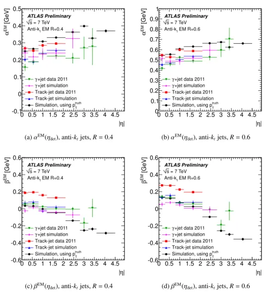
µ. Fig. 4 summarizesα^EM

(η

det

) and

β^EM

(η

det

) derived from track jet and

γ+jet

events, and their dependence on

η_det

.

6.3 E ff ect of out-of-time pile-up in di ff erent calorimeter regions

The decrease of

β^EM

(η

_det

) towards higher

η_det

, as shown in Figs. 4(c) and (d), indicates a decreasing signal contribution to p

^jet_T,EM

per out-of-time pile-up interaction. For jets beyond about

|ηdet| >

1.5, the offset is increasingly suppressed in the signal with increasing

µ

(β

^EM

(η

det

)

<

0). This constitutes a qualitative departure from the behaviour of the pile-up history contribution in the central region of ATLAS, where this out-of-time pile-up leads to systematically increasing signal contributions with increasing

µ.

This is a consequence of two effects. First, for

|ηdet|

larger than about 1.7 the hadronic calorimetry in ATLAS changes from the

Tile

calorimeter to the liquid argon end-cap calorimeter (HEC). The

Tile

calorimeter has a unipolar and fast signal shape [29]. It has little sensitivity to out-of-time pile-up, with an approximate shape signal base line of 150 ns. The out-of-time history manifests itself in this calorimeter as a small positive increase of its contribution to the jet signal with increasing

µ.

The

HEC, on the other hand, has the typical ATLAS liquid argon bipolar pulse shape with approxi-

mately 600 ns baseline. This leads to an increasing suppression of the contribution from this calorimeter to the jet signal with increasing

µ, as more activity from the pile-up history increases the contribution

weighted by the negative pulse shape.

Second, for

|ηdet|

larger than approximately 3.2, coverage is provided by the ATLAS forward calorime-

ter (FCal). While still a liquid argon calorimeter, the

FCal

features a considerably faster signal due to

very thin argon gaps. The shaping function for this signal is bipolar with a net zero integral and a similar

positive shape as in other ATLAS liquid argon calorimeters, but with a shorter overall pulse baseline (ap-

proximately 400 ns). Thus, the

FCal

shaping function has larger negative weights for out-of-time pile-up

of up to 70% of the (positive) pulse peak height, as compared to typically 10

−

20% in the other liquid

argon calorimeters [4]. These larger negative weights lead to larger signal suppression with increasing

activity in the pile-up history and thus with increasing

µ.

(11)

η|

| 0 0.5 1 1.5 2 2.5 3 3.5 4 4.5 [GeV]EMα

-0.1 0 0.1 0.2 0.3 0.4 0.5

+jet data 2011 γ

+jet simulation γ

Track-jet data 2011 Track-jet simulation

truth

Simulation, using pT

= 7 TeV s

EM R=0.4 Anti-kt

ATLAS Preliminary

(a)α^EM(ηdet), anti-ktjets,R=0.4

η|

| 0 0.5 1 1.5 2 2.5 3 3.5 4 4.5 [GeV]EMα

0 0.1 0.2 0.3 0.4 0.5 0.6 0.7 0.8 0.9 1

+jet data 2011 γ

+jet simulation γ

truth

= 7 TeV s

EM R=0.6 Anti-kt

(b)α^EM(ηdet), anti-ktjets,R=0.6

η|

| 0 0.5 1 1.5 2 2.5 3 3.5 4 4.5 [GeV]EM β

-0.6 -0.4 -0.2 0 0.2 0.4 0.6

+jet data 2011 γ

+jet simulation γ

truth

= 7 TeV s

EM R=0.4 Anti-kt

(c)β^EM(ηdet), anti-ktjets,R=0.4

η|

| 0 0.5 1 1.5 2 2.5 3 3.5 4 4.5 [GeV]EM β

-0.6 -0.4 -0.2 0 0.2 0.4 0.6

+jet data 2011 γ

+jet simulation γ

truth

= 7 TeV s

EM R=0.6 Anti-kt

(d)β^EM(ηdet), anti-ktjets,R=0.6

Figure 4: The pile-up contribution per additional vertex, measured as

α^EM = ∂p^jet_T,EM/∂N_PV

, as function

of

|ηdet|

, for the various methods discussed in the text, for R

=

0.4 (a) and R

=

0.6 (b) jets. The

contribution from

µ, calculated asβ^EM = ∂

p

^jet_T,EM/∂µ

and displayed for the various methods as function

of

|η_det|

, is shown for the two jet sizes in (c) and (d), respectively. The points for the MC simulation

based determination of

α^EM

and

β^EM

use the offset calculated from the reconstructed p

^jet_T,EM

and the true

(particle level) p

^truth_T

, as indicated in Eq. 1.

(12)

7 Determining the systematic uncertainties

The systematic uncertainties introduced by applying the MC simulation-based pile-up correction to the reconstructed p

^jet_T,EM

and p

^jet_T,LCW

for jets in collision data include the variation of the slopes

α =

∂

p

T/∂NPV

and

β= ∂

p

T/∂µ

with changing jet p

T

. While the immediate expectation from the stochastic and diffuse nature of the (transverse) energy flow in pile-up events is that all slopes in N

_PV

(α

^EM

,

α^LCW

) and

µ

(β

^EM

,

β^LCW

) are independent of this jet p

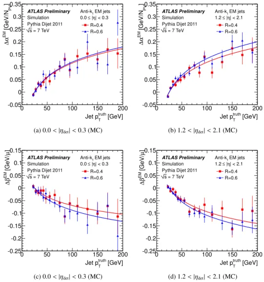
T

, Fig. 5 clearly shows a p

^truth_T

dependence of the signal contributions from in-time and out-of-time pile-up for jets reconstructed on EM scale. A similar p

^truth_T

dependence can be observed for jets reconstructed on LCW scale.

The fact that the variations

∆(∂p_T/∂N_PV

) with p

^truth_T

are very similar for narrow (R

=

0.4) and wide (R

=

0.6) anti-k

t

jets indicates that this p

T

dependence is associated with the signal core of the jet. The presence of dense signals from the jet increases the likelihood that small pile-up signals survive the noise suppression applied in the clustering algorithm. As the core signal density of jets increases with p

_T

, the acceptance for small pile-up signals increases as well, and thus the pile-up signal contribution to the jet increases. This jet p

_T

dependence is expected to approach a plateau as the cluster occupancy in the core of the jet approaches saturation, which means that all calorimeter cells in the jet core survive the selection imposed by the noise thresholds in the topo-cluster formation, and therefore all pile-up scattered into these same cells contributes to the reconstructed jet p

T

. The jet p

T

-dependent pile-up contribution is not explicitly corrected for, and thus is implicitly included in the systematic uncertainty discussed below.

Since the pile-up correction is derived from MC simulation, it explicitly does not correct for system- atic shifts due to mis-modeling of the effects of pile-up on simulated jets. The sizes of these shifts may be estimated from the differences between the offsets obtained from data and from MC simulation:

∆O^EM = O^EM

(N

_PV, µ)

_data− O^EM

(N

_PV, µ) _MC

∆O^LCW = O^LCW

(N

PV, µ)

_data− O^LCW

(N

PV, µ) _MC

To assign uncertainties that can cover these shifts, and to incorporate the results from each in-situ method, combined uncertainties are calculated as a weighted RMS of

∆O

(N

PV, µ) from both theγ+jet and track

jet-based offset measurements. The weight of each contribution is the inverse squared uncertainty of the corresponding

∆O

(N

_PV, µ). This yields absolute uncertainties inα

and

β, which are then translated

to fractional systematic shifts in the fully calibrated and corrected jet p

T

that depend on the pile-up environment, as described by N

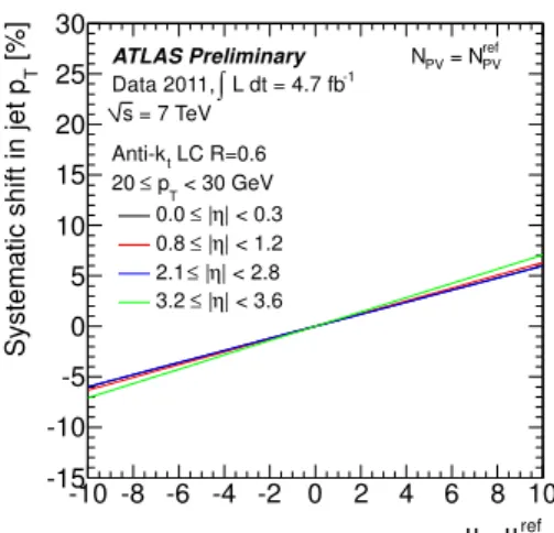
PV

and

µ.

Figure 6 shows the fractional systematic shift in the p

_T

measurement for anti-k

_t

jets with R

=

0.4, as a function of the in-time pile-up activity measured by the displacement

N

PV−

N

_PV^ref

. The shifts are shown for various regions of the ATLAS calorimeters, indicated by

ηdet

, and in bins of the reconstructed transverse jet momentum p

^jet_T,EM+JES

for jets calibrated with the EM+JES scheme (Figs. 6(a), (c)), and (e)). Figures 6(b), (d) and (f) show the shifts for jets reconstructed with the LCW+JES scheme in the same regions of ATLAS and in bins of p

^jet_T,LCW+JES

. The same uncertainty contributions from wider jets reconstructed with the anti-k

_t

algorithm with R

=

0.6 are shown in Figs. 7(a) through 7(f).

Both the EM+JES and LCW+JES calibrations are normalized such that the pile-up signal contribu- tion is 0 for N

PV =

N

_PV^ref

and

µ = µ^ref

, so the fractional systematic shifts associated with pile-up scale linearly with the displacement from this reference. In general, jets reconstructed with EM+JES show a larger systematic shift from in-time pile-up than LCW+JES jets, together with a larger dependence on the jet catchment area defined by R, and the jet direction

ηdet

. In particular, the shift per reconstructed vertex for LCW+JES jets in the two lowest p

^jet_T,LCW+JES

bins shows essentially no dependence on R or

η_det

, as can be seen comparing Figs. 6(b) and 7(b) to Figs. 6(d) and 7(d).

The systematic shift associated with out-of-time pile-up, on the other hand, is independent of the

chosen jet size, as shown in Fig. 8 for R

=

0.4 and Fig. 9 for R

=

0.6. Similar to the shift from in-time

(13)

[GeV]

truth

Jet pT

0 50 100 150 200

] PV [GeV/NEM α∆

-0.05 0 0.05 0.1 0.15 0.2 0.25 0.3 0.35

= 7 TeV s Simulation Pythia Dijet 2011

EM jets Anti-kt

| < 0.3 η

≤ | 0.0 ATLAS Preliminary

R=0.4 R=0.6

(a) 0.0<|ηdet|<0.3 (MC)

[GeV]

truth

Jet pT

0 50 100 150 200

] PV [GeV/NEMα∆

-0.05 0 0.05 0.1 0.15 0.2 0.25 0.3 0.35

EM jets Anti-kt

| < 2.1 η

R=0.4 R=0.6

(b) 1.2<|ηdet|<2.1 (MC)

[GeV]

truth

Jet pT

0 50 100 150 200

]µ [GeV/EM β∆

-0.25 -0.2 -0.15 -0.1 -0.05 0 0.05 0.1 0.15

EM jets Anti-kt

| < 0.3 η

R=0.4 R=0.6

(c) 0.0<|ηdet|<0.3 (MC)

[GeV]

truth

Jet pT

0 50 100 150 200

]µ [GeV/EM β∆

-0.25 -0.2 -0.15 -0.1 -0.05 0 0.05 0.1 0.15

EM jets Anti-kt

| < 2.1 η

R=0.4 R=0.6

(d) 1.2<|ηdet|<2.1 (MC)

Figure 5: The difference from the average

α^EM

(η

det

) of the in-time pile-up signal contribution per re- constructed primary vertex (∆(∂ p

^jet_T,EM/∂N_PV

)(p

^truth_T

)) as a function of the true jet transverse momentum p

^truth_T

, for MC simulated jets reconstructed with anti-k

_t

R

=

0.4 and R

=

0.6 at EM+JES scale, in two different regions

|ηdet| <

0.3 (a) and 1.2

< |ηdet| <

2.1 (b) of the ATLAS calorimeter. The variation of the out-of-time pile-up signal contribution per interaction with p

^truth_T

around its average

β^EM

(η

det

) (∆(∂p

^jet_T,EM/∂µ)(p^truth_T

)) is shown in (c) and (d), respectively, for the same jet samples and

ηdet

regions.

The data points are fit using logarithmic functions of p

^truth_T