Measurements of spin correlation in top-antitop quark events from proton-proton collisions at √

(1)

ATLAS-CONF-2013-101 16September2013

ATLAS NOTE

ATLAS-CONF-2013-101

September 16, 2013

Measurements of spin correlation in top-antitop quark events from proton-proton collisions at √

s = 7 TeV using the ATLAS detector

The ATLAS Collaboration

Abstract

Measurements of spin correlation in top quark pair production are presented using data collected with the ATLAS detector at the LHC with proton-proton collisions at a center- of-mass energy of 7 TeV, corresponding to an integrated luminosity of 4.6 fb

⁻¹

. Events are selected in final states with two charged leptons and at least two jets. Four different observables sensitive to different properties of the production mechanism are used to extract the correlation between the top and antitop quark spins. Some of these observables are measured for the first time. All measurements are in good agreement with the next-to- leading-order Standard Model prediction.

c

Reproduction of this article or parts of it is allowed as specified in the CC-BY-3.0 license.

(2)

1 Introduction

The top quark, discovered in 1995 by the CDF and D0 collaborations at the Tevatron proton-antiproton collider at Fermilab [1, 2], is the heaviest known elementary particle. Besides the high mass, measured to be m

t =

173.20

±

0.87 GeV [3], a distinct feature of the top quark is its short lifetime, determined to be (3.29

⁺_−0.63^0.90

)

×

10

⁻²⁵

s [4], which is shorter than the time scale for hadronization [5]. This implies that top quarks can be studied as bare quarks and the spin information of the top quark can be deduced from its decay products.

In the Standard Model (SM) of particle physics, top quark production at hadron colliders takes place in pairs (t¯ t) via the strong interaction, or singly via the electroweak interaction. At the Large Hadron Collider (LHC), colliding protons with protons ( pp) at a center-of-mass energy of 7 TeV, top quarks are mainly produced in pairs via gluon-gluon fusion. In the SM, t¯ t pairs are produced essentially unpolarized at the LHC [6–8]. Nonetheless, the correlation of the spin orientation of the top and the antitop quark can be studied, and is predicted to be non-zero [8–26].

New physics models beyond the SM (BSM) can change the spin correlation of the top and the antitop quark by either changing the spin of the daughter particles of the top quark, or by changing the production mechanism of the t¯ t pair. The first scenario occurs, for example, if a top quark decayed into a tauonically decaying charged Higgs boson as it is predicted in Supersymmetric (SUSY) models [27,28]. The second scenario occurs, for example, in BSM models where a t¯ t pair is produced via a high-mass Z

⁰

boson with the same couplings to top quarks as the SM Z boson [29] or via a heavy Higgs boson that decays into t¯ t [30]. Thus measuring spin correlation in t¯ t events is important since top quark production and decay can be simultaneously probed for potential new physics e

ff

ects.

The measurements of the spin correlation between the top and antitop quarks presented in this note rely on angular distributions of the top and antitop quark decay products. The charged leptons from the W boson decays are particularly sensitive polarization analyzers. Observables in the laboratory frame and in different top quark spin quantization bases are explored. The extracted physical quantity is the spin correlation strength A which is a measure for the number of events where the top and antitop quark spins are parallel minus the number of events where they are anti-parallel with respect to a spin quantization axis, normalized by the total number of events.

The spin correlation in t¯ t events has been studied previously at the Tevatron and the LHC. The CDF and D0 collaborations have performed a measurement of A by exploring the angular correlations of the charged leptons [31, 32] in dilepton final states. The D0 collaboration has exploited a matrix element based approach [33], and reported first evidence for non-vanishing t¯ t spin correlation [34, 35]. All mea- surements are limited by statistical uncertainties, and are in good agreement with the SM prediction.

Using the difference in azimuthal angle of the two leptons from the decays of the W bosons emerging from top quarks in the laboratory frame,

∆φ, the ATLAS collaboration recently reported first observation

of non-vanishing t¯ t spin correlation using 2.1 fb

⁻¹

of LHC data, taken at 7 TeV collision energy [36]. The CMS collaboration studied spin correlations using the

∆φ

observable as well as the differential angular distributions inclusively and at high m

t¯t

[37].

These measurements as well as those presented here are complementary to the measurements at the Tevatron because the dominant t¯ t production channel at the LHC is gluon-gluon fusion, while at the Tevatron t¯ t production via q q ¯ annihilation dominates.

In this note, the measurements of t¯ t spin correlation using the full 7 TeV data sample of 4.6 fb

⁻¹

,

collected by the ATLAS collaboration are presented. They are performed using the

∆φ

observable, with

revised systematic uncertainties, and the additional observables that are sensitive to different types of

sources of new physics in t¯ t production, such as angular correlations between the charged leptons from

(3)

of the objects and event selection in Secs. 3 and 4, respectively. Section 5 describes the modeling of signal and background contributions and the sample composition. In Sec. 6 the individual observables are described in more detail. The measurement procedure is outlined in Sec. 7, and the sources of systematic uncertainties considered for the measurements are described in Sec. 8. The results are presented in Sec. 9.

Conclusions are given in Sec. 10.

2 The ATLAS Detector

The ATLAS experiment [38] is a multi-purpose particle physics detector. Its cylindrical geometry allows a solid angle coverage close to 4π. ATLAS uses a right-handed coordinate system, with origin at the nominal interaction point in the center of the detector. The z-axis points along the beam direction, the x-axis from the interaction point to the center of the LHC ring, and the

y-axis upwards. In the transverse

plane, cylindrical coordinates (r, φ) are used, where

φ

is the azimuthal angle around the beam direction.

The pseudorapidity

η

is defined via the polar angle

θ

as

η=−

ln tan(θ/2).

Closest to the interaction point is the inner detector, that covers a pseudorapidity of

|η| <

2.5. It consists of multiple layers of silicon pixel and microstrip detectors and a straw-tube transition radiation tracker. Around the inner detector, a superconducting solenoid is constructed, that provides a 2 T axial magnetic field. The solenoid is surrounded by the calorimeter system, consisting of high-granularity lead

/

liquid-argon electromagnetic calorimeters, a steel

/

scintillator-tile hadronic calorimeter in the barrel, and two copper/liquid-argon endcap calorimeters.

The outermost part of the ATLAS detector is the muon spectrometer. It consists of several layers of trigger and tracking chambers. A toroidal magnet system produces an azimuthal magnetic field to enable an independent measurement of the muon track momenta.

A three-level trigger system [39] is used for the ATLAS experiment. The first level is purely hardware-based and is followed by two software-based trigger levels.

3 Object Reconstruction

In the SM, a top quark predominantly decays into a W boson and a b quark. For this analysis t¯ t candidate events are selected where both W bosons emerging from top and antitop quarks decay leptonically into eν

e

,

µν_µ

or

τν_τ

, with the

τ

lepton decaying into an electron or a muon and the respective neutrinos.

Events are required to be triggered by a single electron or single muon trigger with a minimum lepton transverse momentum ( p

_T

) requirement that depends on the lepton flavor and the data-taking period to cope with the increasing instantaneous luminosity. During the 2011 data-taking period the average number of simultaneous pp interactions per beam crossing (pile-up) at the beginning of a fill of the LHC increased from 6 to 17. Events accepted by the trigger are required to have at least one reconstructed hard-scattering vertex with at least three associated tracks, consistent with the beam collision region in the x

−y

plane. The primary hard-scattering event vertex is defined as the vertex with the highest sum of the squared p

_T

values of the associated tracks.

The physics objects considered in this analysis are electrons, muons, jets, and missing transverse

momentum. Electron candidates [40] are reconstructed from energy deposits (clusters) in the electro-

magnetic calorimeter that are associated to reconstructed tracks in the inner detector. They are required

to have a transverse energy, E

_T

, greater than 25 GeV and

|η_cluster|<

2.47, excluding the transition region

1.37

< |η_cluster| <

1.52 between sections of the electromagnetic calorimeters. In addition, electron can-

didates are required to be isolated from other activity in the calorimeter and in the tracking system. An

η-dependent cut based on the energy sum of cells around the direction of each candidate is made for a

cone in

η−φ

space of radius

∆

R

=

0.2, after excluding cells associated with the electron cluster itself.

(4)

An isolation cut is made on the track p

_T

sum around the electron track in a cone of radius

∆

R

=

0.3. The longitudinal impact parameter of the electron track with respect to the event primary vertex, z

₀

, is required to be less than 2 mm. Electrons which are within

∆

R

=

0.4 of a selected jet are removed.

Muon candidates are reconstructed from track segments in various layers of the muon spectrometer, and are matched with tracks found in the inner detector. They are required to be isolated and to have p

_T >

20 GeV and

|η| <

2.5. Isolation cuts include

∆

R

>

0.4 from any selected jet and calorimeter and track isolation. Calorimeter isolation requires that transverse energy within a cone of

∆

R

<

0.2 has to be below 4 GeV after excluding the muon energy deposits in the calorimeter. The track isolation requires the scalar sum of the track transverse momenta in a cone of

∆

R

<

0.3 around the muon has to be less than 2.5 GeV excluding the muon track.

Jets are reconstructed from topological clusters [38,41] built from energy deposits in the calorimeters with the anti-k

t

algorithm [42–44] with a distance parameter R

=

0.4. The jets are calibrated using energy and

η-dependent calibration factors derived from simulations to the mean energy of stable particles inside

the jets. Additional corrections to account for the di

ff

erence between simulation and data are derived from in-situ techniques and applied to data [41, 45].

Calibrated jets with p

_T >

25 GeV and

|η| <

2.5 are selected. To reduce the background from other pp interactions within the same bunch crossing, an additional requirement on the fraction of the sum of the p

_T

of tracks associated with a jet and originating from the primary vertex is imposed. Finally, the jet within

∆

R

=

0.2 closest to a selected electron is discarded to avoid double-counting of electrons as jets.

The missing transverse momentum (E

_T^miss

) is reconstructed from the vector sum of all calorimeter cell energies associated with topological clusters with

|η|<

4.5 [46]. Contributions from the calorimeter clusters matched with either a reconstructed lepton or jet are corrected for the corresponding energy scale. The term accounting for the selected muon p

_T

is included into the E

^miss_T

calculation.

4 Event Selection

To select t¯ t candidate events with leptonic W decays two leptons of opposite charge (`

⁺`⁻=

e

⁺

e

⁻

,

µ⁺µ⁻

or e

^±µ^∓

) and at least two jets are required. For the

µ⁺µ⁻

final state, events containing a muon pair consistent with a cosmic muon signature are rejected. Since the same-flavor leptonic channels e

⁺

e

⁻

and

µ⁺µ⁻

suffer from a large background from the leptonic decays of hadronic resonances, such as the J/ψ and

Υ

, the invariant mass of the two leptons, m

_``

, is required to be larger than 15 GeV. A contribution from the Drell-Yan production of Z/γ

^∗

bosons in association with jets (Z/γ

^∗+jets production) to these

channels is suppressed by rejecting events where m

_``

is close to the Z boson mass:

|m_``−

m

Z|>

10 GeV.

In addition, large missing transverse momentum, E

_T^miss >

60 GeV, is required to account for the two neutrinos from the leptonic decays of the two W bosons in t¯ t events. Drell-Yan events have no neutrinos in the final state and get further suppressed by the E

^miss_T

cut. The e

^±µ^∓

channel does not suffer from an overwhelming Drell-Yan background. For these events no m

_``

or E

^miss_T

cut is applied. To suppress the remaining background from Z/γ

^∗

(

→τ⁺τ⁻

)+jets production a cut on the scalar sum of the transverse energy of leptons and jets, H

_T>

130 GeV, is applied.

5 Sample Composition and Modeling

After event selection backgrounds to dilepton t¯ t production arise from the Drell-Yan Z/γ

^∗+jets produc-

tion with the Z boson decaying into e

⁺

e

⁻

or

µ⁺µ⁻

in the corresponding same-flavor leptonic channels and

with the Z boson decaying into

τ⁺τ⁻

followed by the leptonic decay of

τ

in the e

^±µ^∓

channel. Further

(5)

boson in association with jets. The latter three contain an additional misidentified lepton that does not come from a top quark decay, which can be caused, for example, by jets with a very high electromag- netic component or by genuine leptons inside jets that passed the isolation requirement. Their yield is estimated using data-driven methods.

Drell-Yan events are generated using the A

 

2.13 [47] generator including LO matrix elements with up to five additional partons. The CTEQ6L1 PDF set [48] is used, and the cross section is normal- ized to the NNLO prediction [49]. Parton shower and fragmentation are modeled by H



v6.520 [50], and the underlying event is simulated by J



[51]. To avoid double-counting of partonic configurations generated by both the matrix-element calculation and the parton-shower evolution, a parton-jet matching scheme (“MLM matching”) [52] is employed. The yields of dielectron and dimuon Drell-Yan events predicted by the simulation are compared to the data in Z/γ

^∗+

jets dominated control regions. Correction factors are derived and applied to the predicted yields in the signal region, to account for the difference between simulation prediction and data.

Single top quark background arises from the associated Wt production, when both the W boson emerging from the top quark and the W boson from the hard interaction decay leptonically. This contri- bution is generated with MC@NLO v4.01 [53–55] using the CT10 PDF set [56] and normalized to the approximate NNLO theoretical cross section [57].

Finally, the diboson backgrounds are modeled using A

 

2.13 interfaced with H



using the MRST LO** PDF set [58] and normalized to the theoretical calculation at next-to-leading order (NLO) QCD [59].

The background arising from the misidentified and non-prompt leptons referred to collectively in the following as “fake leptons” is determined using a data-driven technique known as matrix method [60,61].

Signal t¯ t events including SM spin correlation are generated assuming a top quark mass of 172.5 GeV using the MC@NLO v4.01 generator which decays top quarks followed by the W boson decay. It is interfaced with H which showers the b quarks and W-boson daughters and J to simulate multiparton interactions. The CT10 PDF set is used.

The generation chain can be modified such that top quarks are decayed by H



rather than MC@NLO. In this case the top quark spin information is not propagated to the decay products, and therefore the spins between top and antitop quarks are uncorrelated. This technique has a side e

ff

ect that the top quarks in the uncorrelated case are treated as being on shell and hence they do not have an intrinsic width. The effect of this limitation is found to be negligible.

e

⁺

e

⁻ µ⁺µ⁻

e

^±µ^∓

Z(→

`⁺`⁻

)+jets (DD) 21

±

3 83

±

9 — Z(→

τ⁺τ⁻

)

+

jets (MC) 18

±

6 67

±

23 172

±

59 Fake leptons (DD) 20

±

7 29

±

4 101

±

15 Single top (MC) 31

±

3 83

±

7 224

±

17 Diboson (MC) 23

±

8 60

±

21 174

±

59 Total (non-t¯ t) 112

±

13 322

±

33 671

±

87 t¯ t (MC) 610

±

37 1750

±

110 4610

±

280 Expected 721

±

39 2070

±

110 5280

±

290 Observed 736 2057 5320

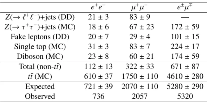
Table 1: Observed events in data compared to the expectation after the selection. Backgrounds and signal estimated from simulation are indicated with the (MC) su

ffi

x, whereas backgrounds estimated using data driven techniques are indicated with a (DD) suffix. Quoted uncertainties include the statistical uncertainty on the yield and the uncertainty on the theoretical cross sections used for MC normalization.

The uncertainty on the DD estimate is statistical only.

(6)

In Table 1 the observed yields in data are compared to the expectation from the background and the t¯ t signal normalized to

σtt¯ =

177

⁺₋₁₁¹⁰

pb calculated at NNLO in QCD including resummation of next-to-next-to-leading logarithmic soft gluon terms with T++ v2.0 [62–67] for a top quark mass of 172.5 GeV. Significantly lower yield in the dielectron channel compared to the dimuon one is due to the tight isolation and higher p

_T

cut on the electrons. The yield di

ff

erence between t¯ t signal with SM spin correlation and without spin correlation is found to be negligible.

6 Spin Correlation Observables

The spin correlation of pair-produced top quarks can be extracted by analyzing the angular distributions of the top quark decay products in t

→

Wb followed by W

→ `ν. The differential distribution of the

decay width

Γ

is given by

1

Γ

d

Γ

d cos

θ± =

(1

+α±

cos

θ±

)/2

,

(1)

where

θ±

is the angle between the positively (negatively) charged lepton from the top (antitop) quark decay and the top (antitop) quark spin quantization axis in the top (antitop) quark rest frame. The factor

α±

represents the spin analyzing power, which can be between

−1 and 1. For positively (negatively)

charged leptons, the spin-analyzing power to the order

αs

is predicted to be

α± = ±0.999 [68]. As a

consequence the dilepton final state offers an excellent sensitivity to analyze t¯ t spin correlation [69]. In the SM, polarization of the pair-produced top quarks in pp scattering is negligible [26]. The correlation between the positively charged lepton and the negatively charged lepton can be expressed by

1

σ

dσ

d cos

θ₊

d cos

θ− =

1 4 (1

+

A

α₊α−

cos

θ₊

cos

θ−

)

,

(2) with

A

=

N

_like−

N

_unlike

N

_like+

N

_unlike =

N(

↑↑

)

+

N(

↓↓

)

−

N(

↑↓

)

−

N(

↓↑

)

N(↑↑)

+

N(↓↓)

+

N(↑↓)

+

N(↓↑) (3)

where N(↑↑)

+

N(↓↓) represents the number of events where the top quark and antitop quark spins are parallel, and N(

↑↓

)

+

N(

↓↑

) is the number of events where they are anti-parallel. The strength of the spin correlation is defined by

C

=−Aα₊α−

(4)

and is the physical observable of interest to measure and to compare to the SM prediction. It is directly related to the expression in Eq. 2 via

C

=−9hcosθ₊

cos

θ−i.

(5)

In this note, however, the full distribution of cos

θ₊

cos

θ−

as defined in Eq. 2 is used. In dilepton final states where the spin-analyzing power is e

ff

ectively 100%, C

≈

A. To allow for a comparison to previous results, in this note the results are given in terms of A.

The following four observables are measured to extract the spin correlation strength:

•

The azimuthal difference

∆φ

between the charged lepton momentum directions in the laboratory

frame. This observable is straightforward to measure and very sensitive at the LHC, where like-

helicity gluon-gluon initial states dominate [70]. It has been utilized in Ref. [36] to observe a

non-vanishing spin correlation, consistent with the SM prediction.

(7)

•

The “S -ratio” of matrix elements

M

for top quark production and decay from the fusion of like- helicity gluons (g

_Rg_R+g_Lg_L →

t¯ t

→

(bl

⁺ν)(¯

bl

⁻ν) ) with SM spin correlation and without spin

¯ correlation at LO [70],

S

=

(|M|

²_RR+|M|²_LL

)

corr

(|M|

²_RR+|M|²_LL

)

uncorr

(6)

=

m

²_t{(t·

l

⁺

)(t

·

l

⁻

)

+

(¯ t

·

l

⁺

)(¯ t

·

l

⁻

)

−

m

²_t

(l

⁺·

l

⁻

)}

(t

·

l

⁺

)(¯ t

·

l

⁻

)(t

·

t) ¯

where t, ¯ t, l

⁺

and l

⁻

are the 4-momenta of the top quarks and the charged leptons. Since the like- helicity gluon-gluon matrix elements are used for the construction of the S -ratio, it is particularly sensitive to like-helicity gluon-gluon initial states. To measure this observable and the two others described below the top and antitop quarks have to be fully reconstructed, which is challenging at a hadron collider.

•

The double differential distribution defined in Eq. 2, in the helicity basis as top quantization axis.

For the helicity basis the top direction in the t¯ t rest frame is used as the quantization axis. As shown in Eq. 2, the measurement of this distribution allows a direct extraction of the spin correlation strength A

_helicity

[8] as defined in Eq. 3. The SM prediction is A

^SM_helicity=

0.31 which was calculated including NLO QCD corrections to t¯ t production and decay and mixed weak-QCD corrections to the production amplitudes in Ref. [26]. Using MC@NLO including only NLO QCD corrections to t¯ t production but not top quark decay, but adding parton showers interfaced by H, the same number is reproduced.

•

The double differential distribution defined in Eq. 2, using the so-called “maximal” basis as top quantization axis. For the gluon-gluon fusion process, which is a mixture of like-helicity and unlike-helicity inital states, no optimal axis exists where the spin correlation strength is 100%.

This is in contrast to the quark-antiquark annihilation process where an optimal “off-diagonal” ba- sis was first identified by Ref. [71]. However, on an event by event basis a quantization axis called

“maximal” basis which maximizes spin correlation can be constructed for the gluon-gluon annihi- lation process [72]. A prediction for the t¯ t spin correlation using this observable does not exist in the literature for a 7 TeV LHC. Therefore, the prediction is calculated using MC@NLO

+

H



simulation resulting in A

^SM_maximal=

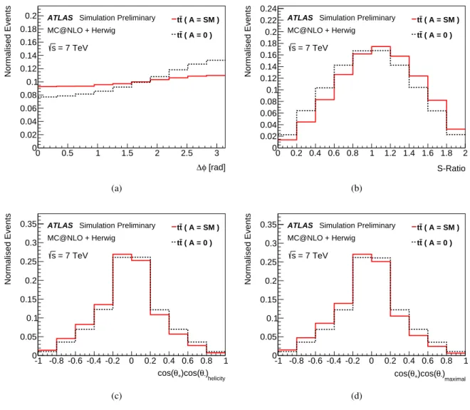
0.44. To illustrate the sensitivity, Fig. 1 shows all four observables for generated charged leptons and top partons before decay, calculated with MC@NLO and interfaced to parton shower generation by H



under the assumption of SM t¯ t spin correlation and no spin correlation, as defined in Sec. 5.

7 Measurement Procedure

After selecting a t¯ t enriched data sample and estimating the signal and background composition as de- scribed in Secs. 4 and 5, the spin correlation observables as defined in Sec. 6 are measured and used to extract the strength of the t¯ t spin correlation.

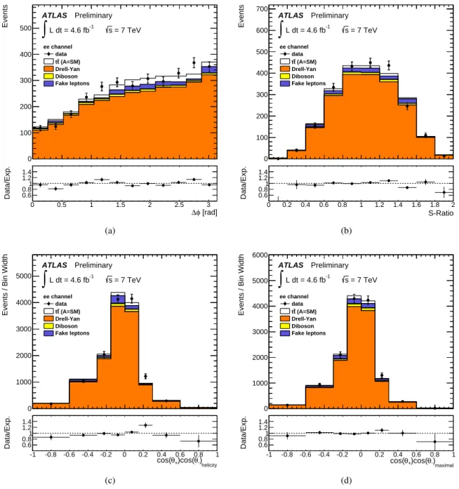
The

∆φ

observable is measured by using the momentum directions of the two leptons in the labo-

ratory frame to calculate the azimuthal angle between them. Figure 2 and 3 (upper left each) show this

distribution in the e

⁺

e

⁻

and

µ⁺µ⁻

channels, respectively, in a control region dominated by Z/γ

^∗+

jets

production. This region is selected using the same requirements as for the signal sample selection, but

inverting the Z mass window cut defined in Sec. 4. The other observables, cos

θ₊

cos

θ−

and the S -ratio,

require the reconstruction of the full kinematics of the t¯ t system since they involve the 4-momenta of the

(8)

[rad]

φ

∆

0 0.5 1 1.5 2 2.5 3

Normalised Events

0 0.02 0.04 0.06 0.08 0.1 0.12 0.14 0.16 0.18

0.2 tt ( A = SM )

( A = 0 ) t t ATLAS Simulation Preliminary MC@NLO + Herwig

= 7 TeV s

(a)

S-Ratio 0 0.2 0.4 0.6 0.8 1 1.2 1.4 1.6 1.8 2

Normalised Events

0 0.02 0.04 0.06 0.08 0.1 0.12 0.14 0.16 0.18 0.2 0.22 0.24

( A = SM ) t

t ( A = 0 ) t t ATLAS Simulation Preliminary MC@NLO + Herwig

= 7 TeV s

(b)

helicity

) θ-

)cos(

θ+

cos(

-1 -0.8 -0.6 -0.4 -0.2 0 0.2 0.4 0.6 0.8 1

Normalised Events

0 0.05 0.1 0.15

0.2 0.25 0.3

0.35 tt ( A = SM )

= 7 TeV s

(c)

maximal -) θ )cos(

θ+

cos(

-1 -0.8 -0.6 -0.4 -0.2 0 0.2 0.4 0.6 0.8 1

Normalised Events

0 0.05 0.1 0.15

0.2 0.25 0.3

0.35 tt ( A = SM )

= 7 TeV s

(d)

Figure 1: Distributions of

∆φ

(a), S -ratio as defined in Eq. 6 (b), cos(θ

₊

) cos(θ

−

) as defined in Eq. 2 in the helicity basis (c) and in the maximal basis (d) for generated charged leptons and top partons before decay using MC@NLO+H at

√

s

=

7 TeV. The normalized distributions show predictions for SM

spin correlation (red solid) and no spin correlation (black dotted).

(9)

top and antitop quarks and of the charged leptons in the laboratory frame and boosts into the top and antitop rest frames, respectively, as can be seen in Eqs. 2 and 6.

For each observable templates are constructed for the background sources and for signal events with SM and without spin correlation in each dilepton subchannel. They are fitted to the data to extract the correlation strength. In this section, first the reconstruction method, and then the fitting procedure are described.

7.1 Kinematic reconstruction of the t t ¯ system

Dilepton final states involve neutrinos from the leptonic W-boson decays. Since neutrinos do not interact with the detector their energy or direction cannot be measured but can only be inferred from the mea- surement of the missing transverse momentum in the event. Since two neutrinos are present, while only the sum of their missing transverse momenta can be measured, the t¯ t system is underconstrained. The t¯ t event reconstruction deals with this problem as well as with the challenge of assigning final state ob- jects to their parent top or antitop quarks by taking advantage of various constraints. The reconstruction method is performed exactly in the same way for data and for simulated events.

In this analysis the method known as the “neutrino weighting technique” [73] is employed. It uses the following constraints for the reconstructed final state objects to solve the event kinematics: the W-boson mass constructed from the charged lepton and neutrino, and the top quark mass equal to the invariant mass of the jet-lepton-neutrino combination. To be able to fully solve the kinematics the pseudorapidities

η₁

and

η₂

of the two neutrinos are taken from a fit of a Gaussian function to the respective distributions in a simulated sample of t¯ t events. It has been checked that the

η₁

and

η₂

distributions in t¯ t events do not change for different t¯ t spin correlation strengths. 50 values are chosen for each neutrino

η, with

−4< η1,2 <

4 taken independently from each other.

Scanning over all

η₁

and

η₂

configurations taken from the simulation, all possible solutions of how to assign the charged leptons, neutrinos and jets to their parent top and antitop quarks are accounted for.

In addition, the energies of all final state jets are smeared according to the experimental resolution [74]

and the solutions are re-calculated for every smearing step. Around 95% of t¯ t events in simulation have at least one solution. This fraction is considerably lower for the backgrounds. To each solution, a weight

w

is assigned, comparing the calculated missing transverse energy from the sum of the two neutrino momenta to the observed one measured either in data or in the simulation. Solutions that fit better to the expected t¯ t event kinematics get a higher weight than solutions fitting worse. The weight is defined by

w= X

η₁,η₂

X

solutions

Y

d=x,y

exp(

−(E^miss,calc_d −

E

_d^miss,obs

)

²

2σ

_Emiss

T

), (7)

where E

^miss,calc_x,y

(E

^miss,obs_x,y

) is the calculated (observed) missing transverse energy component in x or

y

direction. For

σ_Emiss

T

the resolution of the measured missing transverse energy is taken [46]. The weights for all solutions define a weight distribution of each observable per event. For each event the weighted mean value of the respective observable is used for the measurement.

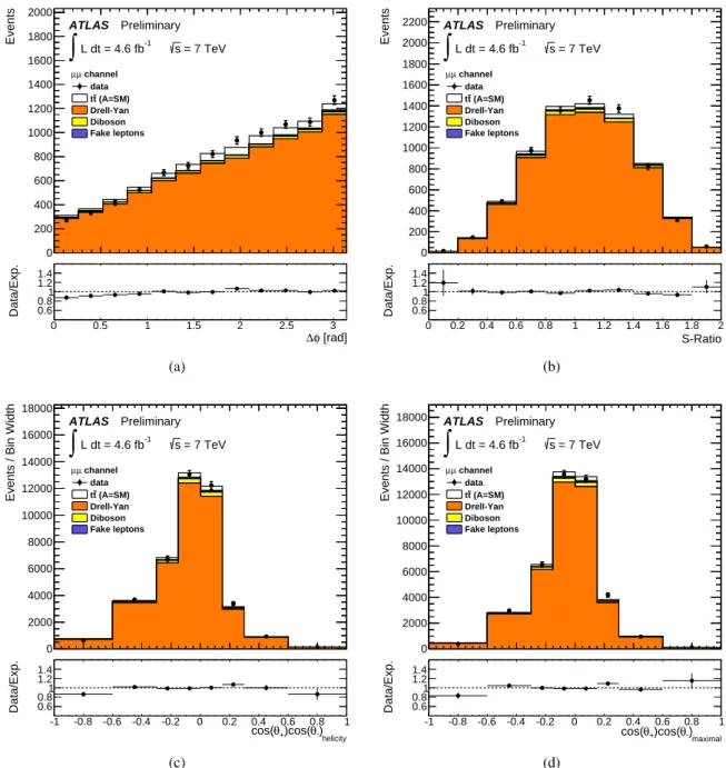
Figures 2 and 3 (b,c,d) show distributions of spin correlation observables that use the t¯ t event re-

construction with the neutrino weighting method. For the e

⁺

e

⁻

and

µ⁺µ⁻

channels, in a control region

dominated by Z/γ

^∗+

jets production, the S -ratio and cos

θ₊

cos

θ−

in two di

ff

erent spin quantization bases

are presented. Good agreement between data and prediction is observed confirming a reliable description

of observables sensitive to t¯ t spin correlations with and without t¯ t event reconstruction in the Drell-Yan

background.

(10)

[rad]

φ

∆

Events

0 100 200 300 400 500

ee channel data

(A=SM) t t Drell-Yan Diboson Fake leptons

ATLAS Preliminary L dt = 4.6 fb-1

∫

^s^{= 7 TeV}

[rad]

φ

0 0.5 1 1.5 2 2.5 ∆ 3

Data/Exp. ^0.6

0.81 1.2 1.4

(a)

S-Ratio

Events

0 100 200 300 400 500 600 700

∫

^s^{= 7 TeV}

S-Ratio 0 0.2 0.4 0.6 0.8 1 1.2 1.4 1.6 1.8 2

Data/Exp. ^0.6

0.81 1.2 1.4

(b)

helicity -) θ )cos(

θ+ cos(

Events / Bin Width

0 1000 2000 3000 4000 5000

∫

^s^{= 7 TeV}

θ+

-1 -0.8 -0.6 -0.4 -0.2 0 0.2 cos(0.4 0.6 0.8 1

Data/Exp. ^0.6

0.81 1.21.4

(c)

maximal -) θ )cos(

θ+ cos(

Events / Bin Width

0 1000 2000 3000 4000 5000 6000

∫

^s^{= 7 TeV}

maximal -) θ )cos(

θ+

-1 -0.8 -0.6 -0.4 -0.2 0 0.2 cos(0.4 0.6 0.8 1

Data/Exp. ^0.6

0.81 1.21.4

(d)

Figure 2:

Distributions of observables sensitive tott¯spin correlation in thee⁺e⁻channel in aZ/γ^∗+jets background dominated control region: The azimuthal angle∆φbetween the two charged leptons (a), theS-ratio as defined in Eq. 6 (b), cosθ₊cosθ−as defined in Eq. 2 in the helicity basis (c) and in the maximal basis (d). TheZ/γ^∗+jets background is normalized to the data in the control region.

(11)

[rad]

φ

∆

Events

0 200 400 600 800 1000 1200 1400 1600 1800 2000

channel µ µ

data (A=SM) t t Drell-Yan Diboson Fake leptons

∫

^s^{= 7 TeV}

[rad]

φ

0 0.5 1 1.5 2 2.5 ∆ 3

Data/Exp. ^0.6

0.81 1.2 1.4

(a)

S-Ratio

Events

0 200 400 600 800 1000 1200 1400 1600 1800 2000 2200

channel µ µ

∫

^s^{= 7 TeV}

S-Ratio 0 0.2 0.4 0.6 0.8 1 1.2 1.4 1.6 1.8 2

Data/Exp. ^0.6

0.81 1.2 1.4

(b)

θ+ cos(

Events / Bin Width

0 2000 4000 6000 8000 10000 12000 14000 16000 18000

channel µ µ

∫

^s^{= 7 TeV}

θ+

-1 -0.8 -0.6 -0.4 -0.2 0 0.2 cos(0.4 0.6 0.8 1

Data/Exp. ^0.6

0.81 1.21.4

(c)

maximal -) θ )cos(

θ+ cos(

Events / Bin Width

0 2000 4000 6000 8000 10000 12000 14000 16000 18000

channel µ µ

∫

^s^{= 7 TeV}

maximal -) θ )cos(

θ+

-1 -0.8 -0.6 -0.4 -0.2 0 0.2 cos(0.4 0.6 0.8 1

Data/Exp. ^0.6

0.81 1.21.4

(d)

Figure 3:

Distributions of observables sensitive tott¯spin correlation in theµ⁺µ⁻channel in aZ/γ^∗+jets background dominated control region: The azimuthal angle∆φbetween the two charged leptons (a), theS-ratio as defined in Eq. 6 (b), cosθ₊cosθ−as defined in Eq. 2 in the helicity basis (c) and in the maximal basis (d). TheZ/γ^∗+jets background is normalized to the data in the control region.

(12)

7.2 Extraction of spin correlation

To extract the spin correlation strength from the distributions of the respective observables in data, tem- plates are constructed and a binned maximum likelihood fit is performed. For each background contri- bution, one template for every observable is made. For the t¯ t signal, one template is constructed from an MC@NLO sample with SM spin correlation and another using MC@NLO without spin correlation.

The templates are fitted to the data, and the fraction of t¯ t events with SM spin correlation,

f

_SM =

N

_A=SM/(N_A=SM+

N

_A=0

)

.

(8)

is extracted. Here N

A=S M

(N

A=0

) is the number of t¯ t events with SM (without) spin correlation. This is equivalent to extracting the spin correlation strength A in a given spin quantization basis as defined in Eq. 3, since any fraction of events with correlated and uncorrelated spins will lead to a linear change of A according to Eq. 2. To reduce the influence of systematic uncertainties sensitive to the normalization of the signal, the t¯ t cross section

σt¯t

is included as a free parameter in the fit.

The predicted number of events per template bin i as function of f

_SM

can be written as m

ⁱ =

f

_SM×

m

ⁱ_A₌_SM+

(1

−

f

_SM

)

×

m

ⁱ_A₌₀+

N_bkg

X

j=1

m

ⁱ_j

(9)

where m

ⁱ_A=SM

and m

ⁱ_A=0

is the predicted number of signal events in bin i for the signal template obtained with the SM MC@NLO sample and with the MC@NLO sample with spin correlation turned o

ff

, respec- tively, and

P^Nbkg

j=1

m

ⁱ_j

is the sum over all background contributions N

_bkg

. Both m

ⁱ_A=SM

and m

ⁱ_A=0

are taken as function of

σtt¯

, which is free to vary in the fit. The negative logarithm of the likelihood function L

−

log(L)

=

N

Y

i=1

P(nⁱ,

m

ⁱ

) (10)

is maximized with

P(nⁱ,

m

ⁱ

) representing the Poisson probability to observe n

ⁱ

events in bin i with m

ⁱ

events expected. The product in Eq. 10 runs over the N bins of the templates. Since all individual chan- nels are constructed to be exclusive, for the combination of all dilepton final states the fit is performed by adding the logarithms of the likelihood function for all channels.

8 Systematic Uncertainties

Systematic uncertainties are evaluated using ensemble tests. For each source of uncertainty new tem- plates corresponding to the respective up and down variation are created for both the SM and the uncor- related spin templates, taking into account the change of the acceptance and shape of the observable due to the source under study. Pseudo-data sets are generated by mixing these templates according to the measured f

_SM

and applying Poisson fluctuations to each bin. Then the nominal and varied templates are used to perform a fit to the same pseudo-data. This procedure is repeated 1000 times for each source of systematics, and the mean of the distribution of differences between the central fit values and the up and down results is quoted as the systematic uncertainty from this source. Systematic uncertainties arising from the same source are treated as correlated between di

ff

erent dilepton channels.

Several classes of systematic uncertainties have been considered: uncertainties related to the detector

model and to t¯ t signal and background models. Each source can affect the normalization of the signal

(13)

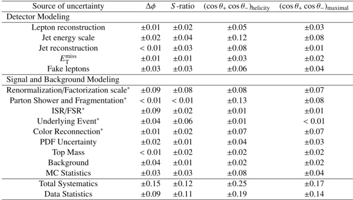
Uncertainties associated with the detector model include uncertainties on the objects used in the event selection. Lepton uncertainties (quoted as “Lepton reconstruction” in Table 2) include trigger e

ffi

ciency and identification uncertainties for electrons and muons, uncertainties due to electron (muon) energy (momentum) calibration and resolution. Uncertainty associated with the jet energy calibration is referred to as “Jet energy scale”, while jet reconstruction e

ffi

ciency and resolution uncertainties are combined and quoted as “Jet reconstruction” in Table 2. Uncertainties on the E

_T^miss

include uncertainties due to the pile-up modeling and the modeling of the energy deposits not associated with the reconstructed objects.

Source of uncertainty

∆φ

S -ratio (cos

θ₊

cos

θ−

)

helicity

(cos

θ₊

cos

θ−

)

maximal

Detector Modeling

Lepton reconstruction

±

0.01

±

0.02

±

0.05

±

0.03 Jet energy scale

±0.02 ±0.04 ±0.12 ±0.08

Jet reconstruction

<

0.01

±0.03 ±0.08 ±0.01

E

^miss_T ±

0.01

±

0.01

±

0.03

±

0.02 Fake leptons

±0.03 ±0.03 ±0.06 ±0.04

Signal and Background Modeling

Renormalization/Factorization scale

^∗ ±0.09 ±0.08 ±0.08 ±0.07

Parton Shower and Fragmentation

^∗ <

0.01

<

0.01

±0.13 ±0.08

ISR

/

FSR

^∗ ±0.09 ±0.02 ±0.01 ±0.01

Underlying Event

^∗ ±

0.04

±

0.06

±

0.01

<

0.01 Color Reconnection

^∗ ±0.01 ±0.02 ±0.07 ±0.07

PDF Uncertainty

±0.02 ±0.01 ±0.04 ±0.03

Top Mass

<

0.01

±

0.02

±

0.02

±

0.02 Background

±0.04 ±0.01 ±0.02 ±0.02

MC Statistics

±0.03 ±0.03 ±0.08 ±0.04

Total Systematics

±0.15 ±0.12 ±0.25 ±0.17

Data Statistics

±

0.09

±

0.11

±

0.19

±

0.14 Table 2: Systematic uncertainties on f

_SM

for the various observables. The accuracy of systematic uncer- tainties requiring a comparison to a second simulation sample is commensurate with the ‘MC Statistics’

uncertainty (see Sec. 8). The corresponding sources of uncertainty are marked by

^∗

.

A number of systematic uncertainties affecting the t¯ t modeling are considered. Systematic uncer- tainty associated with the choice of factorization and renormalization scales in MC@NLO is evaluated by varying the default scales by a factor of two up and down simultaneously. The uncertainty on the choice of the parton shower and hadronization model is determined by comparing two alternative sam- ples simulated with the P



(

 

4) [75] generator interfaced with P



6.425 [76] and H



v6.520. The uncertainty on the amount of initial and final state radiation in the simulated t¯ t sample is

assessed by comparing AMC 3.8 [77] samples interfaced with P with the varied amount of ini-

tial and final state radiation. The size of the variation has been determined from data [78]. The effect

of simulation of the underlying event is estimated by comparing a sample simulated with P



and

showered by P with the P 2011 tune to a sample with the P 2011

H

tune [79]. The

latter is a variation of the P



2011 tune with more semi-hard multiple parton interactions. The impact

of the color reconnection model of the partons that enter hadronization is assessed by comparing samples

simulated with P and showered by P with the P 2011 tune and the P 2011

CR

tune [79]. To investigate the effect of the choice of PDF used in the analysis the uncertainties from the

nominal CT10 PDF set as well as NNPDF2.3 [80] and MSTW2008 [82] NLO PDF sets are considered

and the envelope of the uncertainties of all PDF sets is used to obtain the uncertainty on the measurement.

(14)

The uncertainty from the top quark mass is evaluated by varying its value in the simulation by

±1.4 GeV

which corresponds to the uncertainty on the average top quark mass of m

_t =

173.3

±

1.4 GeV measured at LHC [81].

Uncertainties on the backgrounds (quoted as “Background” in Table 2) evaluated using simulation arise from the limited knowledge of the theoretical cross sections for single top, diboson and Z

→τ⁺τ⁻

production, from the modeling of additional jets in these samples and from the integrated luminosity.

The uncertainty of the latter amounts to

±1.8 % [83]. Systematic uncertainties on the

Z

→

e

⁺

e

⁻

and Z

→µ⁺µ⁻

backgrounds result from the uncertainty of their normalization to data in control regions and modeling of the Z boson transverse momentum. The uncertainty on the fake lepton background (“Fake leptons” in Table 2) arises mainly from uncertainties on the measurement of lepton misidentification rates in di

ff

erent control samples.

Finally, an uncertainty on the method to extract the spin correlation strength arises from the limited statistics to create templates. The systematic uncertainties and their effect on the measurement of f

_SM

are listed in Table 2. Due to the di

ff

erent methods of constructing the four observables, they are di

ff

erently sensitive to the various sources of systematic uncertainty. Some of the given uncertainties are limited by the statistics of the samples used for their extraction. This is not reflected in Table 2.

9 Results

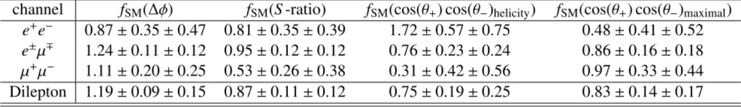
For each of the four observables, the maximum likelihood fit in each of the three individual channels (e

⁺

e

⁻

, e

^±µ^∓

and

µ⁺µ⁻

) and their combination is performed. The observable with the largest statistical separation power between the no spin correlation and the SM spin correlation hypotheses is

∆φ. The

measured values of f

_SM

for

∆φ, the

S -ratio and cos

θ₊

cos

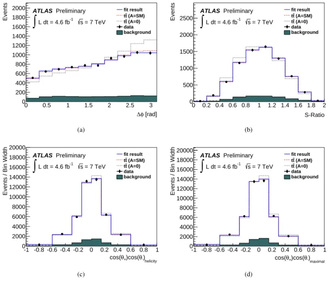
θ−

in the helicity and the maximal bases are summarized in Table 3. Figure 4 shows the observables including the result of the fit to data. Based on statistical uncertainties, the agreement between fit and data is quantified as a

χ²

test per number of degrees of freedom [84] which gives 0.44 for

∆φ, 0.83 for the

S -ratio, 1.03 for cos

θ₊

cos

θ−

in the helicity basis, and 1.60 for cos

θ₊

cos

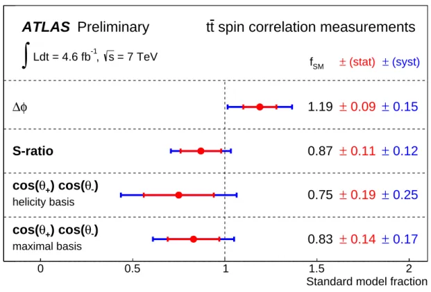
θ−

in the maximal basis. Figure 5 summarizes the measured f

_SM

in the combined dilepton final states for all four observables. All measurements agree with the SM prediction of f

_SM=

1. channel f

_SM

(∆

φ)

f

_SM

(S -ratio) f

_SM

(cos(θ

₊

) cos(θ

−

)

helicity

) f

_SM

(cos(θ

₊

) cos(θ

−

)

maximal

) e

⁺

e

⁻

0.87

±

0.35

±

0.47 0.81

±

0.35

±

0.39 1.72

±

0.57

±

0.75 0.48

±

0.41

±

0.52 e

^±µ^∓

1.24

±

0.11

±

0.12 0.95

±

0.12

±

0.12 0.76

±

0.23

±

0.24 0.86

±

0.16

±

0.18

µ⁺µ⁻

1.11

±

0.20

±

0.25 0.53

±

0.26

±

0.38 0.31

±

0.42

±

0.56 0.97

±

0.33

±

0.44 Dilepton 1.19

±

0.09

±

0.15 0.87

±

0.11

±

0.12 0.75

±

0.19

±

0.25 0.83

±

0.14

±

0.17 Table 3: Summary of f

_SM

measurements in the individual channels and in the combined dilepton channel for the four different observables. The uncertainties quoted are first statistical and then systematic.

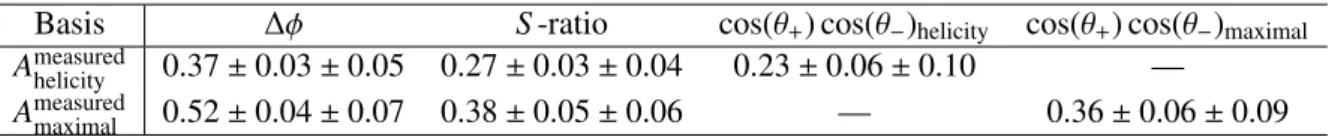
The analysis of the cos

θ₊

cos

θ−

observable allows a direct measurement of the spin correlation

strength A, because A is defined by the cos

θ₊

cos

θ−

distribution according to Eq. 2. In other words,

measuring cos

θ₊

cos

θ−

is equivalent with directly extracting the number of events where the top and

antitop quark spins are parallel minus the number of events where they are anti-parallel, normalized by

the total number of events. This becomes obvious in Eqs. 4 and 5, which show that the expectation value

of cos

θ₊

cos

θ−

is equal to A modulo constant factors. Therefore, the extraction of f

_SM

using the full

(15)

[rad]

φ

∆

0 0.5 1 1.5 2 2.5 3

Events

0 200 400 600 800 1000 1200 1400 1600 1800

2000 _{fit result}

(A=SM) t t

(A=0) t t data background ATLAS Preliminary

L dt = 4.6 fb-1

∫

^s^{= 7 TeV}

(a)

S-Ratio 0 0.2 0.4 0.6 0.8 1 1.2 1.4 1.6 1.8 2

Events

0 500 1000 1500 2000 2500

fit result (A=SM) t t

L dt = 4.6 fb-1

∫

^s^{= 7 TeV}

(b)

θ+

cos(

-1 -0.8 -0.6 -0.4 -0.2 0 0.2 0.4 0.6 0.8 1

Events / Bin Width

0 2000 4000 6000 8000 10000 12000 14000 16000 18000 20000

L dt = 4.6 fb-1

∫

^s^{= 7 TeV}

(c)

maximal

) θ-

)cos(

θ+

cos(

-1 -0.8 -0.6 -0.4 -0.2 0 0.2 0.4 0.6 0.8 1

Events / Bin Width

0 2000 4000 6000 8000 10000 12000 14000 16000 18000 20000

L dt = 4.6 fb-1

∫

^s^{= 7 TeV}

(d)

Figure 4: Distributions of

∆φ

(a), S -ratio (b), cos

θ₊

cos

θ−

in the helicity basis (c) and cos

θ₊

cos

θ−

in

the maximal basis (d). The result of the fit to data (blue) is compared to the templates for background

plus t¯ t signal with SM spin correlation (red dashed) and without spin correlation (black dotted).

(16)

Standard model fraction

0 0.5 1 1.5 2

1.6 7.4

maximal basis

-

) θ ) cos(

θ

+

cos( 0.83 ± 0.14 ± 0.17

helicity basis

-

) θ ) cos(

θ

+

cos( 0.75 ± 0.19 ± 0.25

S-ratio 0.87 ± 0.11 ± 0.12

φ

∆ 1.19 ± 0.09 ± 0.15

ATLAS Preliminary

= 7 TeV s

-1, Ldt = 4.6 fb

∫

spin correlation measurements t

t

fSM ± (stat) ± (syst)

Figure 5: Summary of the measurements of f

_SM